A Multi-Agent Model of Tax Evasion with Public Expenditure

Paolo Pellizzari and Dino Rizzi

A Multi-Agent Model of Tax

Evasion with Public

Expenditure

ISSN: 1827/3580 No. 15/WP/2011

W o r k i n g P a p e r s D e p a r t m e n t o f E c o n o m i c s C a ’ F o s c a r i U n i v e r s i t y o f V e n i c e N o . 1 5 / W P / 2 0 1 1 I S S N 1 8 2 7 - 3 5 8 0

A Multi-Agent Model of Tax Evasion

with Public Expenditure

Paolo Pellizzari

Department of Economics Ca’ Foscari University of Venice

Dino Rizzi

Department of Economics Ca’ Foscari University of Venice

First Draft: October 2011

Abstract

We develop a model where heterogeneous agents maximize their individual utility based on (after tax) income and on the level of public expenditure (as in Cowell, Gordon, 1988). Agents are different in risk aversion and in the relative preference for public expenditure with respect to personal income. In each period, an agent can optimally conceal some income based on conjectures on the perceived probability of being subject to audits, the perceived level of public expenditure and the perceived amount of tax paid by other individuals.

As far as the agent-based model is concerned, we assume that the Government sets the tax rate and the penalties, uses all the revenue to finance public expenditure (with no inefficiency) and fights evasion by controlling a (random) fraction of agents.

We show that, through computational experiments based on micro-simulations, stable configurations of tax rates and public expenditure endogenously form in this case as well. In such equilibrium-like situations we find:

 a positive relationship between the tax rate and evasion still arises.

 tax compliance mainly depends on the distribution of personal features like risk-aversion and the degree of preference for public expenditure.

 an endogenous level of tax evasion that is almost not affected by reasonable rates of control. A proper choice of the tax rate results instead in voluntary partial compliance.

 the enforcement of higher compliance rates requires unrealistic and costly large-scale audits.

Keywords: Tax evasion, public expenditure, agent-based models JEL Codes: H26, H40, C63

Address for correspondence:

Paolo Pellizzari

Department of Economics Ca’ Foscari University of Venice Cannaregio 873, Fondamenta S.Giobbe 30121 Venezia - Italy Phone: (++39) 041 2346924 Fax: (++39) 041 2347444 e-mail: paolop@unive.it

This Working Paper is published under the auspices of the Department of Economics of the Ca’ Foscari University of Venice. Opinions expressed herein are those of the authors and not those of the Department. The Working Paper series is designed to divulge preliminary or incomplete work, circulated to favour discussion and comments. Citation of this paper should consider its provisional character.

The Working Paper Series is available only on line (www.dse.unive.it/pubblicazioni) For editorial correspondence, please contact: wp.dse@unive.it

Department of Economics Ca’ Foscari University of Venice Cannaregio 873, Fondamenta San Giobbe 30121 Venice Italy

1. Introduction

The problem of tax evasion has been always central in the theory of public finance, but its theoretical relevance increased over time. The seminal articles of Allingham and Sandmo (1972) and Yitzhaki (1974) were followed by many contributions which extended and enriched the original model in several ways. Review articles appear periodically to examine the literature and describe a buoyant variety of research lines2.

A particularly important issue is the excessive tax compliance observed in the real world with respect to the level that the standard model of tax evasion would predict3. Another particularly relevant issue is the impact of the level of tax rates on compliance, that in Allingham, Sandmo and Yitzhaki’s works is ambiguous or opposite to what is currently supported by common sense or experimental findings4.

Following Kirchler, Hoelzl and Wahl (2008), other important issues that have been analysed are the impact of audit probabilities, fines, subjective tax knowledge and participation, attitudes toward taxes, personal and social norms, perceived fairness.

Interesting extensions to the standard model are the explicit consideration of labour supply (Cowell, 1985) and of public goods (Cowell and Gordon, 1985).

In many cases, the predictions of the theoretical literature about tax compliance are open to debate as they depends heavily on individual taxpayers’ characteristics, on the institutional framework and on the structure of the social relations.

The necessity to investigate the impact on tax compliance of individual characteristics and interaction in a dynamic framework led to an increasing use of agent-based models that can offer some useful insights through numerical simulations of complex behaviour of heterogeneous agents. The seminal contribution in this field can be traced back to Mittone and Patelli (2000). Using an epidemic-related metaphor, the authors simulate the behaviour of agents whose type is honest, imitative and free rider. The taxpayers derive some utility from the public good and can switch to other types based on a myopic estimate of the their utility. The main result of the paper is that the lack (or insufficient level) of audits induce the spread

1

Paper presented at the conference SHADOW 2011, The Shadow Economy, Tax Evasion and Money

Laundering, Muenster, 28-30/7/2011. 2

See for instance Pyle (1991), Andreoni, Erard, Feinstein (1998), Slemrod, Yitzhaki (2002), Sandmo (2005), Cowell (2003))

of free riders at the expense of honest and fully compliant taxpayers. Many papers have since then adopted approaches where a set of types, endowed with different features, utilities and cognitive/technical abilities, is exogenously assumed to exists. Davis et al. (2003), for example, supports an analytical model with simulations with honest, susceptible and evader taxpayers and find some hysteresis in the reaction to changes in the enforcement system: a compliant population may shift to a state of massive evasion in the presence of too few audits but, in order to reverse the situation, control probabilities must be increased to levels that are higher than the ones that would have kept reasonable compliance in the first place.

Agent based models have the capability to explore several issues that are difficult to deal with in analytical models. Repeated interaction among heterogeneous agents or between the fiscal administration and the taxpayers can be typically addressed by such tools, as well as geographical spillovers and “contagion” effects. The model presented in Korobow et al. (2007) is a recent work where agents are networked in localized structures and are aware of the actions of their neighbours. This social trait of tax evasion may indeed proves itself useful to explain diversity in tax compliance in different regions or environments and reflect the impact of peer-pressure and conformity. Korobow and co-authors find that substantial sharing of payoff information and tax practices can lead to less compliant behaviour. While it is not entirely surprising that one bad apple spoils the whole basket, the result also points out that low “impressionability” of taxpayers may support relative high compliance even with modest auditing levels. The previous result holds when agent ignore the (additional) profit from evasion or information diffusion on tax-related payoffs and misconducts is scarce.

The flexibility of the agent-based methodology can, despite the risk of increasing the number of parameters, allow for great sophistication in the depiction of many realistic features of taxpayers and of the data available to the fiscal authority. Bloomquist (2006) is a good introduction to the field and describes the Tax Compliance Simulator where audit efficacy and celerity, together with a host of other parameters can be changed to test the overall compliance and the success of specific auditing schemes, with regard to both direct and indirect effects (due to additional revenues from fines and increased compliance of other “forewarned” taxpayers, respectively). Bloomquist (2011) builds on some of the previous ideas to present a situated agent-based model with 85000 agents that are calibrated using realistic anonymized public data from the US Internal Revenue Service.

Hokamp and Pickhardt (2010) presents a model with four behaviourally different types, including rational utility maximizers, as in the work of Allingham and Sandmo, and noisy taxpayers who introduce random errors in their reported income. There are also ethical agents

(known as “honest” in other works) and imitators. The latter are located on a ring and report a fraction of the income equal to the average fractions declared by their contiguous neighbours. Such a simplified form of relationship allows for massive interaction and large agents’ number that appears recently in the econophysics literature, such as Zakaln et al. (2009) to pick a representative case. This paper contains a model with 1.000.000 agents on a grid, taking inspiration from the Ising model of ferromagnetism. Taxpayers have “spins” and can be fully compliant (+1) or non-compliant (-1), depending on the state of neighbours and (possibly) on some external force (say, mass media or other biases). As it is typical of similar models, there is a critical “temperature”, that is the degree of social influence, of the system that can trigger phase changes. In spite of some difficulties in the economic interpretation and some questionable assumptions, the model shows that occasional bursts in the evasion rate are possible even under a harsh enforcement system, provided decisions are influenced by the social temperature. See Epstein (2002) for a model of similar acute episodes in a different social context.

In the present paper we develop a model where heterogeneous agents maximize their individual utility based on (after tax) income and on the level of public expenditure. Our agent-based model features utility maximizing heterogeneous taxpayers. The utility is a function of after-tax income, that depends on the reported income, and on the conjectured level of per capita public expenditure. Agents have different risk-aversion coefficients, distinct relative preference for public expenditure and varying trust in the likelihood that others will pay the due amounts. Hence, their final decision rests on micro-founded rational behaviour, personal characteristics and subjective judgements. The enforcement system is based on random auditing and agents exchange information on paid taxes and income levels by randomly meeting other taxpayers. While the two previous components are modelled in a very simple way, we focus on the relevance of the preference for public expenditure to provide different scenarios and equilibrium solutions where the effective tax revenue is exactly what agents conjecture and there is neither under- nor over-provision of public expenditure.

Agents are heterogeneous in risk aversion and in the relative preference for public expenditure with respect to personal income. In each period, an individual can optimally conceal some income based on conjectures on the perceived probability of being subject to audits, the perceived level of public expenditure and the perceived amount of tax paid by other individuals.

We study the optimal behaviour of a single agent, investigate the symmetric Nash equilibrium that arises in a population of homogeneous agents and, finally, perform random simulations to describe a plausible equilibrium in a heterogeneous multi-agents framework.

When analyzing the optimal behaviour of an isolated agent we find that an increase in the tax rate induces more compliance only for low income taxpayers, that is the classic negative relationship between tax rate and tax evasion. On the contrary, high income agents increase their evasion together with the tax rate (for reasonable levels of the tax rate).

A Nash equilibrium in a population of homogeneous agents can be found for any exogenously given tax rate. We find that, depending on the under(over)-provision of public expenditure, two kinds of equilibria are possible. The first one is characterized by low tax rates, under-provision and full compliance, whereas the second one has higher tax rates, over-under-provision and (partial) tax evasion.

As far as the agent-based model is concerned, we assume that the Government sets the tax rate and the penalties, uses all the revenue to finance public expenditure (with no inefficiency) and fights evasion by controlling a (random) fraction of agents.

We show, trough computational experiments based on micro-simulations, that stable configurations of tax rates and public expenditure endogenously form in this case as well. In such equilibrium-like situations we find:

o A positive relationship between the tax rate and evasion still arises.

o Tax compliance mainly depends on the distribution of personal features like risk-aversion and the degree of preference for public expenditure.

o There is an endogenous level of tax evasion that is almost not affected by reasonable rates of control. A proper choice of the tax rate results instead in voluntary partial compliance.

o The enforcement of higher compliance rates requires unrealistic and costly large-scale audits.

The paper is organized as follows. Section 2 describes the model of utility maximization used by the agents. Broadly speaking, the setup is similar to Cowell and Gordon (1988) because public expenditure is considered. Moreover, this section has an extensive sensitivity analysis to study the optimizing agents’ behaviour for different values of relevant parameters. In the third Section, we define and describe the Nash equilibrium arising in a population of homogeneous agents. Finally, the last section attempts to generalize the previous results when heterogeneous agents are considered and interact in a multi-agents computational model.

2. The

Agent

behavior

We consider two types of agents, namely individuals and the Government. Individuals maximize their utility under a fixed monetary income. The utility function depends on the after tax income and on the perceived level of public expenditure. Agents choose the fraction of the income to declare in order to pay income tax. Hence, they have the option to underreport their income to illegally reduce their tax burden.

The Government decides the income tax rate, collects all tax payments and uses all the revenues to provide public expenditure. Therefore, the Government budget is always in balance. Possible inefficiencies in the provision of public goods are not considered.

Government can also contrast tax evasion by controlling a proportion of individuals and by applying a fine on evaded taxes.

Individual agents

Agents face the standard problem of deciding how much of their income to declare for income taxation. Each individual i=1, …, N has a cardinal utility function

[1] U_i U





where yi is the net (after tax) monetary income, Gi is the perceived value of public

expenditure and a_i 





[2]  0   y i U y U and  0   G i U G U

Assumption 2: concavity of utility function:

[3]  0   yy i y U y U ,  0   GG i G _U G U and U_yyU_GG U_yG2 0

Assumption 3: minimum level of utility reached when y_i 0 and G_i 0:

[4] Umin U(0,0)

Assumption 4: minimum level of utility reached when y_i 0 or G_i 0: [5] Umin U(y,0)U(0,G)U(0,0)

One specification that satisfies all previous assumptions is: [6] U





with _y 0,_yy 0, 0_G 0,_GG  and U









, 0_i  is the relative risk aversion parameter and _i 0 represents the relative intensity of individual preference about public expenditure with respect to net income.

With this Cobb-Douglas-type utility function, concavity requires 1_i 1, 1₁(1_i) and 1 ) 1 )( 1 ( 1 i  .

As the parameters _i and _i are chosen by each individual, utility functions are different across individuals.

Income tax and tax evasion control

Income tax is applied, at a constant rate  , to the exogenous amount of income Ii, which is

only known to the taxpayer. Hence, the amount of taxes paid by individual i is:

[8] T_i d_iI_i

where 10di  is the share of gross income declared to Government. Each agent can pick

his di, actually opting for full (di  0), partial (di 0) or no (di 1) tax evasion.

Given the control activity of the Government, each individual faces a probability q of being controlled. If an individual is audited, her tax evasion is certainly discovered and she has to pay a fine of f times the amount of evaded tax:

[9] F_i  f(1d_i)I_i

In the simulations of the model that will be presented in Section 3, individuals do not know exactly the probability of control q, but estimate their own subjective p . i

If the taxpayer is not controlled, his net income is

If the taxpayer is audited, his net income is:

[11] Z(d_i)I_iT_iF_i I_i(1) f(1d_i)I_i

Each individual knows that in aggregate the Government budget constraint holds, therefore the value of public expenditures is equal to total tax revenue:

[12] 



Public expenditure can be decomposed in two parts: the part paid by individual i and the part paid by all others, so that:

[13] Gd_iI_i d_kI_k

k1,ki N



We define the per capita public expenditure financed by all other individuals as:

[14] g ˜ i  1 N1_k1dkIk ki N



When choosing the percentage of income to declare, each taxpayer has to estimate the reaction of other individuals.. This expectation is modelled as a weighted average between the agent’s conjecture about other people’s average tax payment, Ti

~

, and the observed level of per capita public expenditure in the previous period g1. Agent i’s expectation about other people’s average contribution is then:

[16]





We assume the linear form:

[17] g~_i _iT~_i(1_i)g_1

where 10_i  represents the importance of the individual conjecture with respect to other people’s payments with respect to the previous level of public expenditure. If i is close to 0,

then the individual believes that other agents do not react at all (zero conjectural variation)5 and assumes that the per capita spending is constant, whereas as _i approaches 1 it is believed that others will react in the same direction (positive conjectural variation).

Then agent i’s expectation about public expenditure is:

[18]





in which 1ri(N)N is the individual estimate of the degree of rivalness of public expenditure.

We assume that each agent estimates other people’s average tax payment T~_i by using the ratio

i i

i T T

h  ~/ , i.e. an individual estimate of the ratio between Ti

~

and his own tax payment, so that the conjecture of the agent with respect to average payments of other individuals as a response to his contribution is:

[19] T~_i h_iT_i h_id_iI_i

If hi>1 the agent believes that other people pay on average more than him (because, for

instance, they have stronger preferences for public expenditure or higher incomes); when hi=1

the agent conjectures that his payment is equal to the average one and hi<1 implies the belief

that other people pay on average less than him.

Substituting [19] into [17], agent i’s expectation about other people’s average contribution is: [20] g~i ihidiIi (1i)g1.

Hence, the influence of agent i’s tax payment on his expectation about other people’s average payment is: [21] i i i i h T g _   ~

From the above assumptions:





[22] _i i i i i i i i i g N r N g N N I d h N N N N r N G ) ( ) 1 ( 1 1 1 ) ( 1_            _      _ where: [23]       _  _     _   1 1 1(1 )g_1 N N I d h N N N g_i _{i i}  _{i i} _i

is the per capita public expenditure expected by agent i. It is worthwhile noticing that using the utility function [8] the degree of rivalry and the number of individuals are positive constants that cannot change the optimal choice of the agent:

[24] i i i i i i i i i i i i i g N N I d h N N N y N r N U                                 _          1 1 ) 1 ( ) 1 ( 1 1 1 ) ( 1 1

In the case of _i=1, i.e. complete positive conjectural variation, the utility function reduces to: [25]









and hi does not affect the optimal choice.

Utility maximization

The taxpayer chooses the share of income to declare, di, in order to maximise the expexted

utility:

[26] EU(d_i) p_iU_i





[27] ( , ) ( , ) (1 ) ( , ) (1 ) ( , ) 0              i i i i g i i i i i W i i i i i g i i i i i Z i d g g W U p d W g W U p d g g Z U p d Z g Z U p where:









 

i i f I d Z     / i i i i h I N N N d g           / 1 1 i i I d W    /

Obvioulsly, if _i=0 for all agents U_g(y_i,g_i)0 and the standard results of the literature apply6.

The optimal value of d determines the amount of income tax actually paid _i T_i d_iI_i and implicitly the effective tax rate of individual i: _i d_i. The effective tax rate _i can be interpreted as the tax rate that the individual would accept to pay without evading, i.e. his preferred tax rate, given all exogenous variable and parameters, his preferences and conjectures and the control policy of the Government.

In other words, the agent declares all income (d =1) if the statutory tax rate i  is lower than

or equal to his preferred level _i, and will evade some part (1-d )>0 if _i  >_i.

Agent’s comparative statics

The general analysis of the model so far depicted is complex, even if we choose a specific form for the utility function. This is in line with the seminal papers by Allingham-Sandmo (1972) and Cowell-Gordon (1988) where similar models are presented and analytical conclusions were drawn in some cases at the price of strong simplifications.

Our work differs in some respects from the previously mentioned approaches:

1. first of all, under assumptions 1-4, an explicit utility function can be specified. The chosen Cobb-Douglas form exhibits concavity, homogeneity of degree <1 and does not allow for a Ziff (zero income effects) public expenditure;

2. the measure of compliance used in this paper is the fraction of declared income, instead of the level of tax evasion or the level of declared income;

3. we explicitly model the agent’s conjecture about the behaviour of other taxpayers and this will turn out to be an extremely important issue in the subsequent analysis.

4. As in Yitzhaki (1974), penalties depend on the amount of evaded tax.

6

To gain insight in the functioning of the model, we consider a benchmark case whose parameters are listed below.

Table 1 – Benchmark parameters’ values

Number of agents N 1000

Preference for public expenditure  0.5

Relative risk aversion rsion  1.1

Conjecture on other people response  0.5 Conjecture on other people relative tax

paymenth_i T~_i/T_i

h 1

Income I 30000 €

Previous year public expenditure g_1 10000 €

Probability of control p 5 %

Penalty per € of tax evaded f 100%

In the following pictures we consistently use a color code in which low and high values are shown with hues ranging from dark red to bright yellow, respectively. Fig. 1 shows the contours of compliance rate d that maximizes the expected utility function when the two parameters , the relative risk aversion, and  , the relative preference for public expenditure, vary. The compliance rate is zero (the red zone) when both parameter are low, i.e. when the agent has low risk aversion and low preference of public expenditure. When  rises, agents are willing to contribute more and the compliance rate reaches 100% on the right part of the picture.

Fig. 2 shows the contours of compliance rate d that maximizes the expected utility when two important parameters of the enforcement system are changed. As expected, the compliance rate increases with the auditing probability p and with the penalty rate f. The relative effect of the two parameters is different, and compliance is more sensitive to an increment in the control probability p.

Figure 1 – Contours of compliance rate d as a function of utility parameters. 0.0 0.5 1.0 1.5 2.0 012345 alpha rh o 0 .1 0_.2 0 .3 0_.4 0_.5 0 .6 0 .7 0 .8 0 .9

Figure 2 – Contours of compliance rate d as function of evasion control parameters

0.0 0.1 0.2 0.3 0.4 0 .6 0 .8 1 .0 1 .2 1 .4 1 .6 1 .8 2 .0 probability p pe na lt y f 0 .4 0 .4 5 0 .5 0.5₅ 0_.6 0_.6 5 0 .7 0.75 0.8 0.8 5 0_.9 0_.9 5

One of the most important features of tax evasion models is the relationship between tax compliance and increments in the tax rate. Fig. 3 shows that compliance gets bigger with the tax only when income is low. Indeed, at low tax rates, a low-income agent evades almost all

taxes, as the tax and the penalty are small in absolute value and the marginal utility of income is higher than the marginal utility of the exogenously given public expenditure (set to 10000 €). However, increments in the tax rate raise compliance as fines more adversely impact utility of relatively poor agents.

Figure 3 – Contours of compliance rate d as function of tax rate and income

0.2 0.4 0.6 0.8 1.0 2 e + 0 4 4 e + 04 6e+ 04 8e + 0 4 1e+ 05

tax rate tau

in c o m e 0.1 0.2

When income is higher, agents are basically fully compliant for low tax rates, as they are willing to increase tax expenditure relative to income. Compliance first decreases with the tax rate, as public expenditure becomes over-provided but then increases again when the combined effect of taxation and fines kicks in. If evasion is detected when tax rates are higher than 50%, an agent can experience a negative income, due to the 100% penalty and, therefore, there is a strong incentive to avoid such a negative outcome (that nevertheless only occurs for extreme levels of taxation and evasion)

To summarize, the classic and somewhat unrealistic positive relationship between tax rate and tax evasion is found only for low incomes in our setup (for reasonable levels of the tax rate).

3.

Compliance in a population with homogenous agents

Let’s consider a population of N agents with identical incomes and utility functions (see the parameters’ values in Table 1). It is interesting to look at the symmetric equilibrium outcome that emerges when agents are optimizing (and, hence, have no incentive to change their behaviour) and beliefs about the provision of public expenditure are consistent with their observations.

Recall that each agent maximize the expected utility function





)

(d_i p_iU_i Z_i g_i p_i U_i W_i g_i

EU   

in which Z and W are net incomes (whether they are audited or not, respectively) and the conjectured per capita public expenditure is:

      _  _     _   1 1 1(1 )g_1 N N I d h N N N g_i _{i i}  _{i i} _i

We define a Bayes-Nash equilibrium where for each agent the exogenous level of public expenditure g_1 equals the desired level of public expenditure resulting from his utility maximization. So, if d* and g* g_1g_i are the optimal levels for the agents, the Bayes-Nash equilibrium is reached when:

[28]       _  _     _   * * * ) 1 ( 1 1 1 g N N I d N N N

g i  i i i for all agents i=1,…,N

in which we additionally assume that the ratio hi 1

7

. The equilibrium public expenditures are plotted with a thick line in Fig. 4, where the contours of the compliance rate d are plotted as a function of the tax rate and the level of public expenditure g_1.

7

In a symmetric setup, h_i 1 is needed to get a nontrivial Nash equilibrium and, in fact, h_i 1 leads an equilibrium where tax payments are null for all agents.

Figure 4 – Contours of compliance rate d as function of tax rate and g_1 (_i 0.5) 0.2 0.4 0.6 0.8 1.0 0 500 0 1 000 0 1 50 00 20 000 25 00 0 3 000 0

contour of compliance rate d

tax rate tau

exo g e n o u s l e vel of pu b lic expe nd it ur e g (-1 ) 0.1 0.2 0.3

The color code shows that the compliance rate is 100% when exogenous public expenditure and tax rate are low, while the compliance rate decreases rapidly to zero as the exogenous public expenditure increases.

Each point on the blue line shows the equilibrium combination of tax rate, exogenous per capita public expenditure and rate of compliance (contour lines) associated with the Nash equilibrium. Fix, say, a tax rate of 40%: in equilibrium, the corresponding point on the blue line shows that the per capita public expenditure is 6666.67 and agents report d*=57% of their income (incidentally, as 57% is roughly halfway between 0 and 1, the underlying orange hue is roughly halfway between red and yellow).

The dotted bisecting line shows, for each tax rate, the level of per capita public expenditure in a “honest” Nash equilibrium in which we assume that all agents are forced to pay all the amount of taxes required (i.e., if the probability of control is 1).

It is worthwhile to notice that the actual Nash equilibrium line lies on the “honest”, Nash equilibrium in the left lower corner of the picture where both the tax rate and the exogenous public expenditure are low. For higher tax rates the Nash equilibrium line departs from the “honest” benchmark, displaying lower levels of equilibrium public expenditure and decreased compliance, as in the example discussed above.

An examination of the blue line shows, for each tax rate, the level of public expenditure that is generated by agents who optimally underreport their income when the required public expenditure, on the dashed line, is deemed excessive. Observe also that increasing the tax rate is ultimately forcing agents to almost fully comply, but this is again due to the (huge) cost of fines. The level of equilibrium public expenditure is notably flat and very marginally affected by the tax rate in the range 20-50%. In other words, setting a tax rate of 20%, with no tax evasion, produces a per capita public expenditure that is only slightly smaller than the level that would be obtained at 45% where agents underreport in equilibrium, “thinking” that an unreasonable tax burden is required.

The agent-based simulations of the next section will show that this result robustly holds in a non-symmetric environment populated by heterogeneous agents where, “forcing” taxpayers to pay too much (in so doing accepting or perceiving an excessive public expenditure), is costly and requires a harsh enforcement system.

Clearly, equilibria depend on the values (more generally, distributions) of agents’ features, like the preference parameter  . Figure 5 depicts several equilibrium outcomes related to several levels of  . As expected, higher preferences for public expenditure (i.e., higher  ) result in larger endogenous provision in equilibrium.

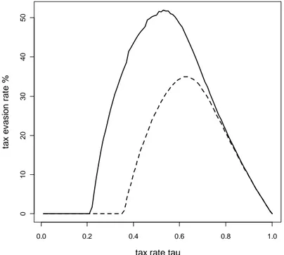
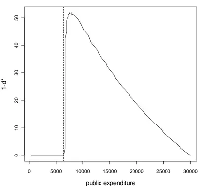
Fig. 6 shows that the tax evasion rate in equilibrium varies as tax rate increases, but it decreases when the tax rate reaches 50%, for the reasons explained above. When the tax rate is low there is no tax evasion: an equilibrium with low tax rate and low public provision is a situation of under-provision of public expenditure and, really, there would be agents ready to pay more than the statutory tax rate. As the rate of compliance is constrained in the range [0,1], the rate of evasion is zero. This situation of under-provision is maintained until the tax rate reaches a level, 21%, that secures the desired level of public expenditure. Further increments of the tax rate push agents to hide of their income because they feel an over-provision of public expenditure. The optimal level of public expenditure, 6300, can be found by looking at the level reached when the evasion rate start to depart from zero (see the vertical dotted line in Fig. 7). This statement can be understood by looking at Figure 8 where the level of utility (that is social welfare as all individuals are homogeneous) are shown. It can be seen that the maximum is achieved at the same public expenditure as in Figure 7 (dotted line) and at the corresponding tax rate.

Figure 5 – Contours of compliance rate d as function of tax rate and g_1 (i 0.5, 75i 0. i 1.0) 0.2 0.4 0.6 0.8 1.0 0 500 0 1 0 000 15 000 20 000 250 00 300 00

contour of compliance rate d

tax rate tau

e x og en ous l e v e l of pub lic ex p e n d it u re g( -1 ) 0.1 0.2 0.3

Figure 6 – Nash equilibrium tax evasion rate as function of tax rate

(_i 0.5, solid, and _i 1.0, dashed)

0.0 0.2 0.4 0.6 0.8 1.0 0 1 02 03 0 4 05 0

tax rate tau

ta x evasi o n r a te %

Figure 7 – Nash equilibrium tax evasion rate as function of g_1 0 5000 10000 15000 20000 25000 30000 0 1 02 03 0 4 05 0

Nash tax evasion rate %

public expenditure

1-d*

Figure 8 – Utility levels at Nash equilibrium

0.0 0.2 0.4 0.6 0.8 1.0 -3 .2 -3 .0 -2 .8 -2 .6 -2 .4

Nash utility level

tax rate tau

Na s h u tilit y 0 5000 10000 15000 20000 25000 30000 -3 .2 -3 .0 -2 .8 -2 .6 -2 .4

Nash utility level

public expenditure Na s h u tilit y

4.

Compliance in a population with heterogeneous agents

The results of the previous section can be generalized in a context of heterogeneous agents who differ about their utility function parameters, risk aversion and relative preference for public expenditure.

We assume that agents are able to decide rationally their best action in term of compliance rate, but do not know exactly some information about the probability of auditing and the amount of taxes actually paid by other people.

Each agent collects the necessary information by meeting a limited number of other individuals. In particular, we assume that in each period each individual meets a fixed number of other agents and exchange some information.

From the meeting the agent can learn:  if the other agent has been controlled  the amount of taxes they effectively paid

Instead, agents do not exchange information about the owed amount of taxes and about the degree of compliance.

The analytical treatment of this heterogeneous agents model is impossible, to the best of our knowledge. Therefore, we simulate a framework in which agents interact and dynamically reach an equilibrium, if it exists, in which the level of public expenditure and the rate of compliance become stable.

As the population is composed by heterogeneous agents, the Nash equilibrium can be defined as the situation in which:

[29]                 * * * ) 1 ( 1 1 1 g N N I d h N N N

g _i_i  _{i i} _i for all agents i=1,…,N

In this case, as agents differ in some parameters, we cannot assume that the ratio h is unitary _i as in the previous section. Actually, if we have, for instance, just two individuals with different income, then it is likely that the richer (R) will pay a higher absolute value of tax than the other (P), so that hR TP/TR 1 and hP TR/TP 1. Hence, h ’s could not be the i

same for all individuals and a Nash equilibrium will arise only if the vector of h ’s will _i converge to a set of compatible values. For this reason, we assume that each agent should

Estimate of the subjective probability of control

An agent meets n other agents in each period and can count how many of them have been controlled (n ). From this information the agent estimates a subjective probability of control: ic

n

n_ic/ . As the Government can change the true probability at any time, the agent re-estimates the subjective probability in each period, and we assume that the value used in the individual utility maximization is a weighted average of his previous estimate (with weight  ) and the new estimate n_ic/ (with weight n 1). So the subjective probability of control of the i-th agent is: [30] n n p p c i t i it  ,1(1)

Estimate of other people contribution to public expenditure

We define the parameter h as the ratio of the average amount of taxes paid by his matches _i and his own payment. We assume furthermore that the value used in the utility maximization is a weighted average of the previous period estimate (with weight ) and the new one (with weight 1): [31] i i i J j j j t i t i I d I d n h h     



where J(i) is the set of agents that i meets at time t (which is omitted for notational simplicity).

Auditing policy

Auditing policy is purely random. In each period a share q of all agents is randomly controlled.

Government

In order to endogenize the public policy parameters, we introduce Government as an additional agent with the following tasks:

- provision of public good and services to be financed by the tax revenue;

- evasion control policy: choice the fraction q of individuals to control and the fine rate f to punish tax evaders.

From the maximisation of his expected utility each individual derives his preferred tax rate, so the Government democratically chooses the income tax rate accepted by the majority of voters, assuming tax payers reveal their preferred tax rate in some voting mechanism. Applying the standard median voter model, the tax rate can be set at the median of the distribution of individual effective tax rate:

[32] ) median(_i

With respect to the evasion control policy, we assume that Government has chosen a fine rate by comparing the punishment for tax evasion to those for other offenses, so that f is an exogenous parameter in the model. Therefore the policy can rely only on the choice of the number of audits, i.e. the share q. As we assume that Government aims to provide the tax rate preferred by the majority of voters (and therefore the corresponding level of public expenditure, because the government budget must be in balance), the share q can be set at a level such that the level of income declared on average by taxpayers is sufficiently high. Being hard to completely eradicate tax evasion, we assume that Government set a target threshold of average income declared, d . Government then rises the number of audits if d <mean(d ), while decreases q if _k d >mean(d ), where _k d is the percentage of declared _k income of the k-th taxpayer audited. If q’ is the variation of q in a period, then:

[33]             ) ( ) ( 1 1 k k d mean d d mean d if q q if q q q

Logical phases of simulation

The simulation is performed in four “logical” phases:  1st

phase: the Government set an arbitrary high tax rate and does not control for tax evasion. In this phase each agent pays the preferred amount of taxes in order to maximize his utility function by computing the optimal compliance rate d.

 2nd

phase: through a voting procedure a new tax rate is set by Government. The new tax rate is the median of preferred tax rates. There is still no control of tax evasion.  3rd

 4th

phase: the Government check the average level of compliance of controlled agents and changes the number of controls in order to reach target threshold of average income declared, d .

Table 2 show the values of parameters used in the simulations.

Table 2 – Values of parameters used in the simulations

Number of agents N 1000

Number of matchings per agent n 10% N

Preference for public expenditure  uniform [0.0, 1.0[

Relative risk aversion  uniform [0.0, 2.2]

Conjecture on other people response  uniform [0.0, 1.0]

Income I Lognormal

mean: 30000 € Standard deviation of log: 2

Previous year public expenditure g_1 0 €

Probability of control q Phase I: 0 %

Phase II: 5.0 % Phase III: endogeneous with

q’=0.5% Initial subjective probability of control p ,...,₁ p_N 0% Initial subjective estimate of other people

contribution to public expenditure trol

N

h

h ,...,1 1

Penalty per € of tax evaded f 100%

weight  in h _i  0.5

weight  in p _i  0.5

One period of the simulation evolves according to the following steps :

1. Agents inherit previous period parameters, maximize utility to decide the tax compliance and pay taxes;

2. Government provides public expenditure, performs random control of taxpayers and punishes tax evaders;

3. Agents gather information meeting other peers and revise estimates of the probability of control and of other agents’ tax payments.

Results

The following figures show some results of one arbitrary simulation that, obviously, cannot represent the full range of possible outcomes.

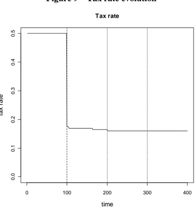
In Figure 9, depicting the evolution of the tax rate, it can be seen that the statutory rate stabilizes quickly at the median value of 16.04%, starting from the second phase of the simulation.

In a related fashion, public expenditure (Figure 10) converges to the average values of 3816 in the second phase (without auditing) and to 3827 in the third phase (where 5% of taxpayers are audited). It is apparent that the proper choice of the tax rate generates a tax revenue that is only mildly lower than the one produced by the introduction of auditing.

At the same time, the average compliance rate (Figure 11) increases from 74.00% to 76.46%. These results represent somewhat the Nash equilibrium values with heterogeneous agents. As the distributions of agents’ parameters have been chosen so that their means match the values of Table 1, we can compare the findings in the two cases.

From these exercises, we can see that the equilibrium tax rate and public expenditure levels are lower in the heterogeneous setting. Indeed, the equilibrium tax rate drops to 16.04% from 21% and public expenditure falls from 6300 to about 3800.

Figure 9 – Tax rate evolution

0 100 200 300 400 0. 0 0 .1 0. 2 0 .3 0. 4 0 .5 Tax rate time ta x r a te

Figure 10 – Public expenditure evolution 0 100 200 300 400 4000 5000 6000 7000 8 000 time publ ic ex pendi tu re

Figure 11 – Tax compliance evolution

0 100 200 300 400 0. 0 0 .2 0. 4 0 .6 0. 8 1 .0 time d

As shown in Figure 12, in the fourth phase the Government must increase the audit probability to about 35% in order to achieve a compliance rate of 90%. Such a level of control

is clearly unrealistic and suggests that the target compliance rate is hard to attain even if more sophisticated auditing schemes.

Figure 12 – Probability of control evolution

0 100 200 300 400 0. 0 0 .1 0. 2 0 .3 time q

5. Concluding

remarks

From the model and the simulation of the paper some interesting conclusions can be drawn. First of all we would like to stress that even in a highly heterogeneous society, in which taxpayers differ in many fundamental aspects (such as risk aversion, preference for public expenditure, conjecture about other people’s compliance) equilibrium-like situations still arises. As the tax rate has been set in an endogenous way (with a median voter procedure), the dynamic of the model lead to situations in which a majority of taxpayers is willing to fully complain given reasonable levels of probability of control and size of fines, while a minority evade at different levels.

The second finding is that individual characteristics (such as the preference for public expenditure with respect to individual income and risk aversion) are much more significant than auditing policy parameters to determine individual compliance. In fact, once that the median voter tax rate is set by the Government, only very high (and unrealistic) levels of the

probability of control can induce individuals with low risk aversion and low preference for public expenditure to reduce their tax evasion.

Finally, we find that the presence of public expenditure can assure a positive relationship between the tax rate and tax evasion without assuming tax morale, social stigma or non-standard individual preferences.

References

Allingham, Michael. G., & Sandmo, Agnar (1972) “Income Taxation: A Theoretical Analysis”, Journal of Public Economics, 1, pp. 323-338.

Andreoni, James, Brian Erard, & Jonathan Feinstein (1998) “Tax Compliance”, Journal of Economic Literature, XXXVI, June, pp. 818-860.

Bloomquist, Kim M. (2006), ‘A Comparison of Agent-Based Models of Income Tax Evasion’, Social Science Computer Review, vol. 24(4), pp. 411-425.

Bloomquist, Kim M. (2011), Agent-Based Simulation of Tax Reporting Compliance, mimeo, Shadow 2011, Muenster.

Bernasconi, Michele, (1998) “Tax Evasion and Orders of Risk Aversion”, Journal of Public Economics, 67, pp. 123–134.

Bernasconi, Michele, & Zanardi Alberto (2003) “Tax Evasion, Tax Rates, and Reference Dependence”, FinanzArchiv, 2004, vol. 60, no. 3, pp. 422-45.

Cornes, R. & Sandler T. (1986) The Theory of Externalities, Public Goods and Club goods, Cambridge University Press, Cambridge.

Cowell, Frank. A. (1985) “Tax evasion with labour income”, Journal of Public Economics, Vol. 26, Issue 1, pp. 19-34

Cowell, Frank. A. (2003) Sticks and Carrots, Discussion paper no. DARP 68 (Distributional Analysis Research Programme, Toyota Centre), London.

Cowell, Frank. A. & Gordon J.P.F. (1988) “Unwillingness to Pay”, Journal of Public Economics, 36, pp. 305-321.

Davis, Jon S., Hecht, Gary & Perkins, Jon D. (2003), “Social Behaviors, Enforcement and Tax Compliance Dynamics”, Accounting Review, vol. 78(1), pp. 39-69.

Epstein, Joshua M. (2002) Modeling civil violence: An agent-based computational approach, PNAS vol. 99, May 14, 2002, p. 7243-7250.

Hokamp, Sascha & Pickhardt Michael (2010), “Income Tax Evasion in a Society of Heterogeneous Agents – Evidence from an Agent-Based Model”, International Economic Journal, 24(4), 541-553

Kirchler, Erich, Hoelzl Erik & Wahl Ingrid (2008) “Enforced versus voluntary tax compliance: The slippery slope framework”, Journal of Economic Psychology , vol. 29, pp. 210-225.

Korobow, Adam, Johnson, Chris & Axtell, Robert (2007) “An Agent-based Model of Tax Compliance with Social Networks”, National Tax Journal, vol. 60(3), pp. 589-610. Mittone, Luigi, & Patelli Paolo (2000). Imitative behaviour in tax evasion. In B. Stefansson &

F. Luna (Eds.), Economic simulations in swarm: Agent-based modelling and object oriented programming, pp. 133-158, Amsterdam: Kluwer.

Pyle, D.J. (1991) “The Economics of Taxpayer Compliance”, Journal of Economic Surveys, vol. 5, no. 2, pp. 163-198.

Sandmo, Agnar (2005) “The Theory of Tax Evasion: A Retrospective View”, National Tax Journal, LVIII, 4, pp. 643-663.

Slemrod, Joel & Shlomo Yitzhaki (2002) “Tax Avoidance, Evasion, and Administration”, in Auerbach A.J. and M. Feldstein, Handbook of Public Economics, Volume 3, Chapter 22, pp. 1423-1470.

Yitzhaki, Shlomo (1974) “A Note on Income Tax Evasion”, Public Finance Quarterly, 15, 2, pp. 123-137.

Zaklan, Georg, Westerhoff Frank & Stauffer Dietrich (2009) "Analysing Tax Evasion Dynamics via the Ising Model", Journal of Economic Interaction and Coordination, Springer, vol. 4(1), pages 1-14, June.