Titolo
l
os
s of core integr
i
ty
i
n a lFR system
:
mode
ls and pre
l
iminary numerical analysis
Ente emittente CIRTEN
PAG
I
NA
DI
GUARDIA
Descrittori
Tipologia del documento: Collocazione contrattuale:
Rapporto Tecnico
Accordo di programma ENEA-MSE: tema di ricerca "Nuovo nucleare da fissione"
Generation IV Reactors
Termoidraulica dei reattori nucleari
Analisi diSicurezza Argomenti trattati:
Sommario
This report, carried out at the Dipartimento di Ingegneria Meccanica, Nucleare edella Produzione (DIMNP) ofthe
University ofPisa in collaboration with ENEA Bologna Research Centre, illustrates preliminary numerical results and the
model for fuel dispersion ina LFR reactor types, i.e. the MYRRHA FASTEF reactor.
The first part ofthis work shows the generalities and the historical background ofthe SIMMER-1I1 code and some relevant
integrai applications. Inthis context the SIMMER-[[1 code is able tobe implemented insafety analysis of sodium-cooled fast
reactors, lead and LBE-cooled fast reactors and also with some limitations inmolten salt reactors and light water reactors. The second part focuses on MYRRHA-FASTEF modelled by SIMMER-[[l, highlighting howeach component was
represented. The reactor was simulated by a two-dimensional R-Zgeometry with 38x89 celi mesh. After this introductive
part conceming the description of the set-up modeI, steady state and transient results are reported.
Steady state condition occurs about twenty seconds after the start ofthe simulation and this report shows the most relevant results obtained for temperature trends andprofiles, both in thecore and in thePHX, and for velocity and mass flow rate. Preliminary transient results were analyzed, i.e. during anUnprotected Loss OfFlow (ULOF) accident, and results were
compared with those obtained with aRELAP5 code. A fuel dispersion transient was also simulated, comparing the effect of
fuel porosity on the fuel dispersion inside the pool
Note
PAR2011 LP3-D4.A. Autori
M. Eboli, I.Angelo, N. Forgione, (UNIPI) G. Bandini (ENEA) Copia n. In carico a: 2 NOME FIRMA 1 NOME FIRMA O EMISSIONE 18/09/20
11
.
NOME M. T~rl:lnt!Do ~VV~
FIRMAREV. DESCRIZIONE DATA CONVALIDA
NA
/VVV\J
Loss of core integrity in a LFR system:
models and preliminary numerical analysis
(Perdita di integrità del nocciolo in un sistema LFR:
modelli e analisi numerica preliminare)
M. Eboli, I. Angelo, N. Forgione
(DIMNP – Università di Pisa)
G. Bandini
(ENEA – Bologna)
Pisa, August 2012
Lavoro svolto in esecuzione dell’Attività LP3-D4
AdP MSE-ENEA sulla Ricerca di Sistema Elettrico - Piano Annuale di Realizzazione 2011 Progetto 1.3.1 “Nuovo Nucleare da Fissione:
2
INDEX
SUMMARY ... 3
1 GENERALITIES AND HISTORICAL BACKGROUND OF THE SIMMER-III CODE ... 4
1.1 Structure model ... 7
1.2 Neutronics model ... 9
1.3 Fluid-dynamics model ... 9
2 INTEGRAL REACTOR APPLICATIONS ... 12
2.1 Lead cooled reactors ... 12
2.2 Sodium cooled reactors ... 16
2.3 Molten salt reactors ... 18
2.4 Light water reactors ... 20
3 DESCRIPTION OF MYRRHA FASTEF AND MODELLING ... 23
3.1 Core modelling ... 24
3.2 Primary cooling system modelling ... 27
3.2.1 Reactor vessel ... 27
3.2.2 Diaphragm ... 28
3.2.3 Core barrel ... 29
3.2.4 Primary heat exchangers ... 30
3.2.5 Primary pump ... 31
4 STEADY-STATE RESULTS ... 32
4.1 Temperature ... 32
4.2 Velocity ... 35
4.3 Mass flow rate ... 36
5 TRANSIENT RESULTS ... 38
5.1 Unprotected loss of flow transient ... 38
5.2 Fuel dispersion analysis ... 41
5.2.1 Forced circulation in the primary circuit ... 42
5.2.2 Natural circulation in the primary circuit ... 46
6 CONCLUSIONS ... 49
REFERENCES ... 50
NOMENCLATURE ... 51
3
was represented. The reactor was simulated by a two-dimensional R-Z geometry with 38x89 cell mesh. After this introductive part concerning the description of the set-up model, steady state and transient results are reported.
Steady state condition occurs about twenty seconds after the start of the simulation and this report shows the most relevant results obtained for temperature trends and profiles, both in the core and in the PHX, and for velocity and mass flow rate.
Preliminary transient results were analyzed, i.e. during an Unprotected Loss Of Flow (ULOF) accident, and results were compared with those obtained with a RELAP5 code. A fuel dispersion transient was also simulated, comparing the effect of fuel porosity on the fuel dispersion inside the pool.
4
1
GENERALITIES AND HISTORICAL BACKGROUND OF THE SIMMER-III
CODE
The consequences of postulated Core Disruptive Accidents (CDAs) have been a major concern in the safety of Liquid-Metal Fast Reactors (LMFRs), because of the energetics potential resulting from a recriticality event. Mechanistic simulation of an accident sequence during a CDA is required to realistically assess the energetics potential and this is only achieved by using a comprehensive computational tool that systematically models coupled multi-phase thermohydraulic and space-dependent neutronic phenomena. In this area, the SIMMER-II code was developed by Los Alamos National Laboratory (LANL) between 1974 and 1986 as the first practical tool of its kind, and has been used in many experimental and reactor analyses. The code has played a pioneering role in the advancement of the mechanistic simulation of CDAs, but at the same time extensive worldwide code application revealed many limitations due to the code framework as well as needs for model improvement. For this reason, the development of a new code, has been initiated in a common effort of PNC (now JNC), CEA, FZK. Between 1986 and 1988, AFDM was developed, a prototype fluid-dynamic two-dimensional code with three velocity fields that will develop into the SIMMER-III code. In 1993 a first version of the code was published with the implementation of the fluid-dynamic models and was followed in 1996 by a new version which added a space-time-dependent neutron kinetics model. The end of the version code and the validation phases were concluded in 2000.
The purpose of SIMMER-III is to alleviate many of the limitations of SIMMER-II and, thereby, to provide a more reliable tool for the analysis of CDAs. The development of the code reached a milestone that all original models sought for, are available for broad use. In order to apply SIMMER-III to LMFR safety analysis, the code must be demonstrated to be sufficiently robust and reliable, and to have been tested and validated extensively. Thus, the code development community performed a systematic assessment program of the code in two steps: “phase 1” for fundamental or separate-effect code assessment of individual models; and “phase 2” for integral code assessment of key physical phenomena relevant to accident analysis.
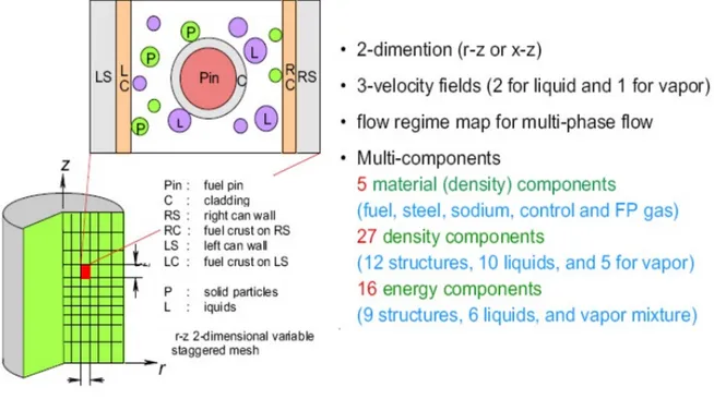
SIMMER-III is a two-dimensional (2-D), three-velocity-field, multi-phase, multi-component, Eulerian, fluid-dynamics code coupled with a fuel-pin model and a space-time and energy-dependent neutron kinetics
model. The conceptual overall framework of the code is shown in
Figure 1.1. The entire code consists of three elements: the fluid-dynamics model, the structure model and the neutronics model. The fluid-dynamic portion, which constitutes about two thirds of the code, is interfaced with the structure model through heat and mass transfer at structure surfaces. The neutronics portion provides nuclear heat sources based on the mass and energy distributions calculated by the other code elements [1].
5
Figure 1.1: Overall framework of SIMMER-III code.
The SIMMER-III code deal with five basic LMFR core materials for each one the operator can choose a different sub-material:
• Fuel (MOX, UO2, C-100, C-84, C-50, C-22, MSRE, MSBR ), • Steel (SUS316),
• Coolant (sodium, water, lead, LBE) • Control material (B4C)
• Fission cas (Xe, Air).
A material can exist in different physical states, so the operator can choose between 7 different phases (for example fuel needs to be represented by fabricated pin fuel, liquid fuel, a crust refrozen on structure, solid particles and fuel vapour, although fission gas exists only in the gaseous state). Thus material mass distributions are modelled by 27 density components in the current version of SIMMER-III, 12 for solid phase, 10 for liquid phase and one for vapour phase. The energy distributions are modelled by only 16 energy components since some density components are assigned to the same energy component, 9 for solid phase, 6 for liquid phase and only 1 for the vapour phase (see Figure 1.2).
Table 1.1: SIMMER-III fluid dynamics structure field components.
Density component (MCSR) Energy component (MCSRE)
s1 Fertile Pin Fuel Surface Node S1 Pin Fuel Surface Node s2 Fissile Pin Fuel Surface Node
s3 Left Fertile Fuel Crust S2 Left Fuel Crust s4 Left Fissile Fuel Crust
s5 Right Fertile Fuel Crust S3 Right Fuel Crust s6 Right Fissile Fuel Crust
s7 Cladding S4 Cladding
s8 Left Can Wall Surface Node S5 Left Can Wall Surface Node s9 Left Can Wall Interior Node S6 Left Can Wall Interior Node s10 Right Can Wall Surface Node S7 Right Can Wall Surface Node
6
s11 Right Can Wall Interior Node S8 Right Can Wall Interior Node s12 Pin Control Surface Node S9 Pin Control Surface Node
Table 1.2: SIMMER-III fluid dynamics liquid field components.
Density component (MCLR) Energy component (MCLRE)
l1 Liquid Fertile Fuel L1 Liquid Fuel l2 Liquid Fissile Fuel
l3 Liquid Steel L2 Liquid Steel
l4 Liquid Sodium L3 Liquid Sodium
l5 Fertile Fuel Particles L4 Fuel Particles l6 Fissile Fuel Particles
l7 Steel Particles L5 Steel Particles
l8 Control Particles L6 Control Particles
l9 Fertile Fuel Chunks L7 Fuel Chunks
l10 Fissile Fuel Chunks
l11 Fission Gas in Liquid Fuel l12 Fission gas in Fuel Particles l13 Fission Gas in Fuel Chunks
Table 1.3: SIMMER-III fluid dynamics vapour field components. Density Component (MCGR) Material Components (MCGM1)
g1 Fertile Fuel Vapour G1 Fuel Vapour
g2 Fissile Fuel Vapour
g3 Steel Vapour G2 Steel Vapour
g4 Sodium Vapour G3 Sodium Vapour
g5 Fission Gas G4 Fission Gas
The structure field components, which consist of fuel pins and can walls, are immobile. Both simple and detailed fuel-pin model is provided, where the fuel pellet is represented by two or several radial temperature nodes, respectively. The mobile components, which include liquids, solid particles and vapours, are assigned to one of three velocity fields (two for liquids and one for vapour), such that the relative motions of different fluid components can be simulated. Although SIMMER-III is tailored to LMFR materials, the thermophysical properties and equation-of-state (EOS) functions are sufficiently flexible for non-LMFR materials to be modelled as well.
7
Figure 1.2: Multi-phase, multi-component fluid-dynamics model in SIMMER-III.
1.1
Structure model
The structure model represents the configuration, and time-dependent disintegration, of the fuel pins and subassembly can walls. Two can walls can be modelled, at the left and right mesh-cell boundaries, each of which contains two temperature nodes. The presence of a can wall at a cell boundary prevents radial fluid convection, and provides a surface where fuel can freeze or vapour can condense. The breakup of structure components is currently based on thermal conditions, simple temperature and wall thickness threshold for mechanical breakup. Both a simple fuel-pin model, where the fuel pellet is represented by two temperature nodes and a sophisticated model to calculate pin failure, fuel-pin radial heat conduction, fission-gas plena modelling and molten central cavity description are available.
The axial geometry of the simplified fuel pin model is shown in Figure 1.3, which simulate a typical LMFR fuel pin structure. The upper and lower axial blanket regions and upper and lower fission gas plenum regions can be placed above and below the active fuel zone. The same configuration can be used for a control pin, as well, but two types of pins cannot co-exist in a same mesh cell.
The radial fuel pin geometry is shown in
Figure 1.4. The pin fuel is modelled by two temperature nodes, while the thin cladding is represented by one node. The surface pin fuel node (as the surface can wall node) has a thickness of thermal penetration length determined from the input structure time constants specified for fuel or steel, as follows:
,
3
2
M2
M Str M Mc
Mκ τ
δ
ρ
=
where
κ
M ,ρ
M andc
M are thermal conductivity, density and specific heat, respectively of material (1 for fuel and 2 for steel). These properties are evaluated by the EOS functions with assuming the solidus energies. The input structure time constant are specified by input. The thermal penetration lengths are calculated only once in the code during initialization and stay constant during the transient calculation. Thus the selection ofτ
Str M, should be made considering the time scale of the problem being calculated.8
The temperature point of the pin fuel interior is placed at the volume centroid. The cladding, or the pin fuel surface node when cladding is missing, undergoes heat and mass transfer with fluid, whereas the pin fuel interior is not directly coupled with the fluid.
Figure 1.3: Axial fuel pin representation in SIMMER-III.
Figure 1.4: Radial fuel pin cross section in SIMMER-III.
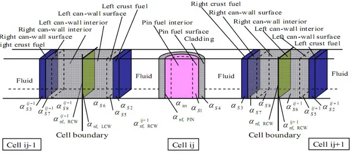
The radial can wall geometry over three successive mesh cells, ij-1, ij, and ij+1, is shown in Figure 1.5. Each can wall is represented by two nodes, the surface and interior, and the temperatures are calculated at the volume centroid of the nodes. The thickness of a surface node is determined from the thermal penetration length of steel. In the standard option, the can wall is represented by a slab geometry to simulate the hexagonal subassembly wrapper tubes. An option is also available to model the can wall by a cylindrical geometry, to simulate, for example, a tube wall in some experimental analysis.
At each mesh cell boundary, two can walls can be placed at the same time, together with the non-flow volumes in between, to simulate inter-subassembly gaps in a reactor. A normal can wall is regarded as “thick” and is modelled by the surface and interior nodes. When the wall becomes “thin”, the wall can no longer be modelled by two nodes and is represented by a single interior node.
For fluid flows, the can wall structures provides a channel wall for an axial flow, and no radial flow across the cell boundary is permitted as long as one of two can walls is present. The can wall exchanges heat and mass with fluid in a mesh cell, and no inter-cell heat transfer is permitted when two walls are present at the cell boundary. However, when one of the two can walls goes missing, then inter-cell heat transfer is calculated. This is done by setting a fraction of the interior node to be a surface node over in an adjacent cell. For example, let us consider the right boundary of a cell ij, where a thick right can wall is presented and the left can wall in a cell ij+1 is missing. Three can wall nodes, S7 and S8 in cell ij, and S5 in cell ij+1, are defined in this case. The surface node in cell ij, S7, undergoes heat and mass transfer with fluid in cell ij, while the surface node in cell ij+1, S5, undergoes heat and mass transfer with fluid in cell ij+1. The three can wall nodes are coupled in the structure heat transfer calculations.
9
Figure 1.5: Fuel pin and can wall configuration in a mesh cell.
1.2
Neutronics model
The space-time-dependent neutron kinetics model in SIMMER-III is based on an improved quasi-static method with a diffusion acceleration technique where the flux shape is calculated by a standard Sn neutron transport theory based on TWODANT. Since the changes in material number densities and temperatures are crucial, a cross-section model is included in the code to perform self-shielding operations to determine effective macroscopic cross sections whenever the reactivity is updated. SIMMER can treat neutronic systems not only with but also without, external source.
1.3
Fluid-dynamics model
The material density and energy component distributions are obtained by solving the mass, momentum and energy conservation equations using three velocity fields. The three-velocity-field formulation and the fluid convection solution algorithm are based on the time-factorization approach which has also been applied and tested for the former AFDM code. In this approach, intracell interfacial area source terms, momentum exchange functions and heat and mass transfer are determined separately from inter-cell fluid convection. A semi-implicit procedure is used to solve inter-cell convection on an Eulerian staggered mesh. Fluid-convection is treated in an explicit, pressure propagation within an implicit scheme. A higher order differencing scheme is also implemented to improve the resolution of fluid interfaces by minimizing numerical diffusion. Higher order differencing proved to be necessary especially in treating interaction type phenomena as fuel coolant interactions. This solution procedure of separating intra-cell transfers from fluid convection is believed to be the most practical for complex multi-component systems like SIMMER-III. This approach had far-reaching implications for the code’s development. Firstly, new models could be easily implemented and added, secondly, computer running times, especially for the three-dimensional version, could be kept at a very low level.
The basic geometric structure of SIMMER-III is a 2-dimensional R–Z system, although optionally an X–Z or one-dimensional system can also be used for various fluid-dynamics calculations. The code models three velocity fields (two for liquids and one for vapour) to simulate relative motions of different fluid components. This allows us to adequately simulate the inter-penetration of melt into coolant. The
three-10
velocity-field formulation of fluid convection in SIMMER-III is based on AFDM. The list of the liquid and vapour-field components used in the present FCI simulations is shown in Table 1.4. The fuel and steel components are assigned to the two material components which comprise the molten mixture. The assignment of fluid components to the three velocity fields is also shown in Table 1.4. The present selection is made such that the relative motion of molten mixture with coolant can be simulated. The densities of solid particles are normally close to those of the melt liquid phases and hence the solid particles are assigned to the same velocity fields as the melt liquid phases rather than the liquid coolant. The vapour species are assumed to be completely mixed and a single energy is assigned to the vapour field.
Table 1.4: Velocity fields.
Phase Velocity Fields Name Symbol
Liquid
q1
Liquid Fertile Fuel l1
Liquid Fissile Fuel l2
Fertile Fuel Particles l5
Fissile Fuel Particles l6
Fission Gas in Liquid Fuel l11 Fission Gas in Fuel Particles l12 Fission Gas in Fuel Chunks l13
q2
Liquid Steel l3
Liquid Coolant l4
Steel Particles l7
Control Particles l8
Fertile Fuel Chunks l9
Fissile Fuel Chunks l10
Gas q3
Fertile Fuel Vapour g1
Fissile Fuel Vapour g2
Steel Vapour g3
Coolant Vapour g4
Fission Gas g5
In this case mass and energy conservation equations are solved for nine density components and six energy components, respectively, in order to model complex flow situations during FCIs [2]. The following conservation equations involving fluid mass, momentum and internal energy are solved:
• mass conservation equation
(
)
m q mv m tρ
ρ
∂ + ∇ ⋅ = −Γ ∂ r • momentum equation(
)
(
)
(
)
(
)
' ' ' ' ' ' ' ' q q q q q q q q m q q qS qq m q q q q qq qq qq q v v v p g K v K v v VM t H v H vρ
ρ
α
ρ
∈ ∂ + ∇ ⋅ + ∇ − + − − − = ∂ = Γ Γ + −Γ ∑
∑
∑
r r r ur r r r uuur r r11
the inter-cell solution. A higher-order differencing scheme is also implemented to improve the resolution of fluid interfaces by minimizing numerical diffusion.
Selection of time step sizes is a very important element of controlling the fluid-dynamics calculations. This is because a sufficiently strict time step control is essential for making the numerical calculation accurate and stable. In addition, practical control is always required from the computing-cost point of view. In SIMMER-III, time step controls are implemented and they automatically select the most appropriate time step size.
12
2
INTEGRAL REACTOR APPLICATIONS
The first integral application of SIMMER-III to the CDA assessment was successfully performed for a typical LMFR of an intermediate size, as reported by Tobita [3].
Nowadays the integral applications are performed for LMFR (both sodium and lead or LBE cooled) but also for molten salt reactor and light water reactor, with some code implementations.
As example, one application for type of reactor is reported below.
2.1
Lead cooled reactors
For this type of reactors, the steady-state and transient analysis of the European Facility for Industrial Transmutation (EFIT) performed by KIT in 2010 [4] is reported. The EFIT is a 400 MW ADS transmuter loaded with a CERCER U-free fuel.
In SIMMER-III simulations, the fuel assemblies have been subdivided into 6 fuel rings in the core, with each zone including two fuel rings. The first three radial meshes are used to represent the target region. The
core is surrounded by outer dummy and absorber assemblies. The primary pump head can be well represented in the simulation through the pump model in SIMMER-III. The heat exchanger in SIMMER-III modelling has been taken into account by defining a proper heat sink to assure that the temperature at the
core inlet is 400°C. To major details see the Figure 2.1a.
In steady state conditions (shown in
Figure 2.1b), the SIMMER-III simulated peak temperature is 1340°C while the peak clad temperature is 520°C, that simulate the design values reasonably well.
Figure 2.1: SIMMER-III model of EFIT and axial temperature profile in the first fuel ring.
The transient cases that were simulated by SIMMER-III are the beam trip, the beam overpower, the protected and unprotected transient overpower, the protected and unprotected loss of flow, and the protected and unprotected coolant flow blockage accident. Unprotected is synonymous with a beam on condition during the accident, while protected means a beam off condition.
13
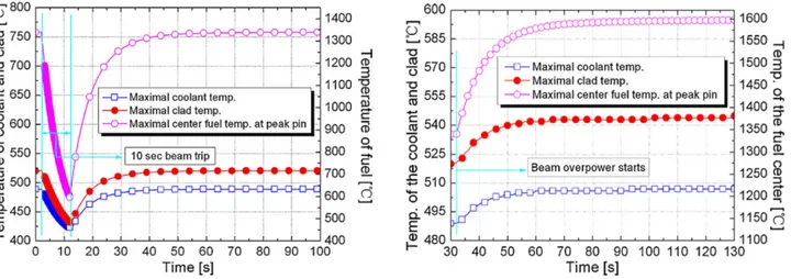
Figure 2.2: Temperature transients in the BT case and in the beam overpower.
In the case of Beam Trip (BT) it is assumed that the beam trip starts 2 seconds after the initial steady state and lasts 10 seconds. When the transient starts, the power decreases at 6.5% of its initial value and rises
again when the beam is on again. The temperature transient is shown in
Figure 2.2a. The maximal fuel, clad and coolant temperature drops by 743, 88 and 65°C, respectively, all within the safety limits.
The beam overpower is assumed to start 2 seconds after the initial steady state. In this transient the core power increases and arrives at a stable value of 20% increase compared to its initial value. The maximal
temperature of the fuel, clad and coolant reaches 1597, 545 and 507°C respectively, safely under the temperature limits (see
Figure 2.2b).
Unprotected Transient OverPower (UTOP) has been triggered 2 s after its initial steady state (see Figure 2.3a), the power increases until a new stabilized state of 21% higher than previously. The final stabilized maximal temperatures of fuel, clad and coolant are 1530, 538 and 503°C respectively, which are
way off their corresponding failure temperature limits. Concerning the Protected Transient OverPower (PTOP), the beam is assumed to be off 3 s after the insertion of reactivity, so power increases only in these
first seconds. The maximal temperature of fuel, clad and coolant, shown in Figure 2.3b, is 1380, 524 and 492°C respectively, which is lower than the previously case.
Figure 2.3: Temperature transients in the UTOP and PTOP cases.
ULOF starts at 2 s counting from its initial steady state. When the pump suddenly stops within 1 s, there is an undershooting of the coolant mass flow rate in the core. As shown in
14
Figure 2.4a this phenomena leads to the overshooting of power and temperature. With the 30% remaining coolant heat removing capacity, the fuel, clad and coolant peak temperatures finally stabilized at 1552, 730 and 685°C respectively, with a peak due to the overshooting of 1687, 884 and 858°C, respectively.
In the case of Protected Loss Of Flow (PLOF), instead, the peak temperature is lower than in the ULOF case, due to the continual decrease of the mass flow rate following the beam off (
Figure 2.4b).
Figure 2.4: Temperature transients in ULOF and PLOF cases.
The Unprotected Blockage Accident (UBA) represents a possible path to core damage. It is a classical accident in the area of severe accident analysis and traditionally played a significant role in safety assessment and licensing. Because the SIMMER-III is a 2D code, the blockage is simulated by coherently
blocking a ring in the fuel assemblies. In the transient shown in
Figure 2.5a, a total blockage at the inner core in the first fuel ring is simulated. The blockage starts 5 s later than its initial steady state. When clad temperature reaches 1007°C, gas blow out starts through cracks in the clad. The break up is assumed to occur at around 1230°C. With the removal of the clad, fuel pellets in
the pin are assumed to be movable. The temperature of the wrapper of the adjacent fuel assemblies increases and the wrapper melts and the fuel of the first fuel ring escapes from the blocked channel to its
neighbouring gap channel, initiating the failure propagation. In the first three rings the melt occurs, because fuel is not easily swept out (see
Figure 2.5a). With the failure of the third fuel ring, more area is available for fuel escaping from the core, so power decreases and no more fuel rings will fail later on. Instead, in the Protected Blockage Accident (PBA)
case, the peak temperatures of fuel, clad and coolant are much lower than the corresponding failure limits due to the power decrease after the beam off (
15
16
2.2
Sodium cooled reactors
One of the most recent reports in literature about the application of the code in a Sodium Fast Reactor (SFR) is performed by Yamano in 2009 [5]. Because SIMMER-III was applied early to SFR, in literature it is possible to find various applications of the code, and recently also the implementation of a new three-dimensional code SIMMER-IV.
In the simulation, the initial condition is based on the best estimated scenario obtained by the SAS4A initiating-phase analysis. Figure 2.6 shows horizontal and vertical geometries used in the SIMMER-IV calculation together with the SAS4A geometry of a 1/3 sector model of the core. The calculation was carried out using the computation meshes of 28 x 29 x 55 = 44660. In the vertical direction only 12 meshes were used for the core.
Figure 2.6: SFR Geometry in SIMMER-IV simulation.
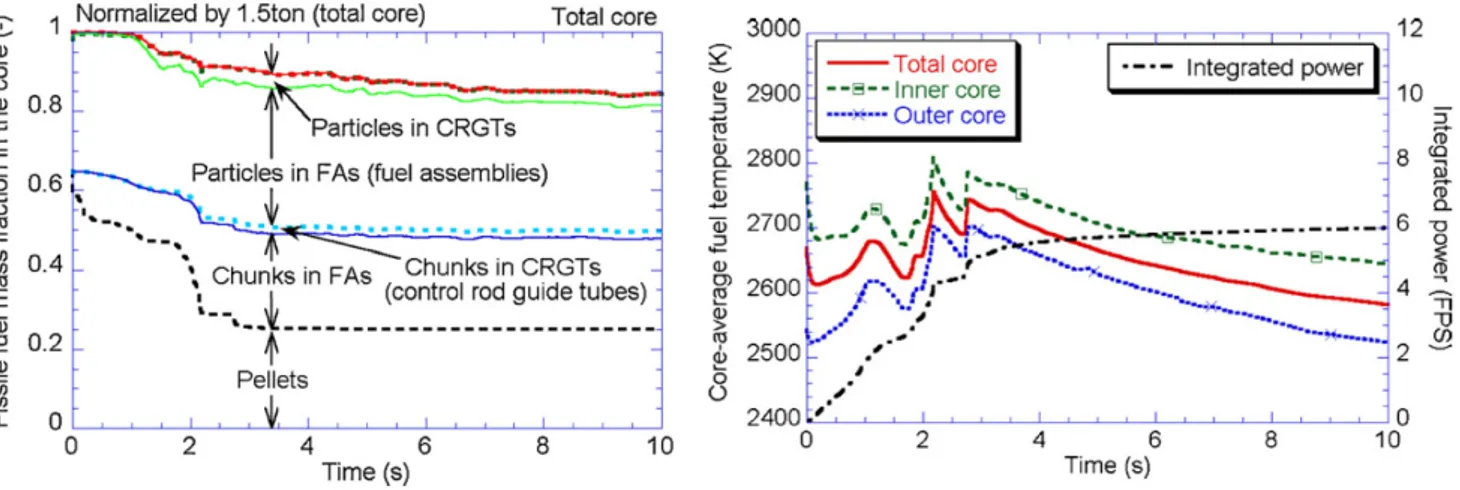
Figure 2.7a presents calculated reactivity and reactor power. The power increase just after the beginning of the calculation occurs as a result of fuel fall-down by gravity in fuel assemblies, where fuel pellets have already been disrupted. The fuel mass in the core decreases due to successive fuel discharge from the core
(
Figure 2.7b). It will be noted that the reactivity decrease tendency is in good agreement with the decrease of fuel mass in the core. In spite of the reduction of fuel mass in the core, reactivity increase can be observed because fuel accumulates at the lower part of the core.
17
Figure 2.7: Reactivity, power and fuel mass fraction in the core. As shown in
Figure 2.8a, the quantity of mobile fuel components increases from about 40% to 65%, which can increase fuel sloshing potential in the inner core, because the major stationary fuel pellets remain in the outer side.
The maximum value of total-core-average fuel temperature is 2755 K (
Figure 2.8b). The temperatures tend to decrease because of heat loss principally to steel components.
Figure 2.8: Fuel components and average fuel temperature in the core.
The disruptive core relocation at the end of the transition phase in the simulation is drawn in Figure 2.9, which may be given as an initial condition of the post-accident material relocation and heat removal phase studies. Although the fuel pellets in most outer core regions are still intact, most of the fuel pellets are disrupted and accumulate in the lower part of the core. The disruptive core contains pellets in the lower part of the upper axial blanket fuel region, thereby contributing to dilution of the fissile core.
18
Figure 2.9: Disruptive core relocation.
2.3
Molten salt reactors
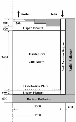
Recently, in the European Union, molten salt reactor technology has been taken into consideration because of its ability to greatly long life waste due to high burn up and on-site simplified processing and the potential to transmute minor actinides [6]. In Russia, a new molten salt reactor concept, MOSART, has been developed (see Figure 2.10).
The geometrical model of SIMMER-III for the MOSART is illustrated in Figure 2.11. The basic assumption of the present simulation is two-dimensional circular-symmetric geometry. The fluid dynamical mesh points are 20 x 30 in R-Z. The neutronic mesh is 60 x 90 where most fluid dynamics meshes are subdivided into three neutronic mesh intervals.
The essential feature of molten salt reactors is the liquid fuel circulating in the core region and in the external primary loop. Due to the very distinctive nature of the circulating fluid fuel, the fissile materials are no longer only confined in the core, but circulate through the heat exchangers and the pumps in the loop, so they spend a part of circulation time outside of the core. In this condition there is a strong correlation between the neutronics in the core and the operating conditions, for instance, a fraction of the delayed neutrons is emitted outside the core.
19 Figure 2.10: 2400 MWth MOSART preliminary design
configuration.
Figure 2.11: MOSART geometric model for SIMMER-III analysis.
The original SIMMER-III neutron computation framework deals only with solid fuel and does not account for precursor movement. In this case, the motion of the molten salt cannot be neglected in writing the precursor equations because the time scale of the convective motion is of the same order as that one of the precursor decays. So, a new model for delayed neutron precursor movement is implemented. Also the thermo fluid-dynamic part has to be extended, to simulate the primary loop behaviour, as one-dimensional. The first simulation was done for the MOSART core configuration without an inlet distribution plate at the bottom of the core, but these results were inconsistent. So, a distribution plate with non-constant orifice coefficients in the bottom plenum was introduced.
Figure 2.12 shows the 2D velocity distribution in the simulation with a properly designed distribution plate. Note that the vector scale is 10. It can be seen that the reverse flow region that appeared in the simulation without plate, in this case disappeared. Figure 2.13 gives the corresponding temperature distribution of the molten salt. In this case the maximal temperature region is located near the reactor core outlet region, and furthermore, the maximal molten salt temperature is about 1150 K. The safety margin has improved.
20
Figure 2.12: Velocity vector distribution. Figure 2.13: 2D Temperature distribution.
So, the SIMMER-III is also capable to be applied to molten salt reactor, with some extension in neutronic and fluid dynamic model.
2.4
Light water reactors
SIMMER-III code is applied in specific LWR areas such as core disruption phenomena and steam explosion. The thermo-hydraulic validation has already occurred; in fact many basic experiments of the “phase-1” and “phase-2” program assessment have been recalculated using water as simulating liquid [7].
More extensions of the code are ongoing, especially in the neutronic model. Heterogeneities appears in the resonance region through the absorption by heavy isotopes, leading to dips in the flux spectra much more pronounced in the fuel than in the no-fuel regions. This phenomenon, neglected in LMFR, cannot be neglected in thermal neutron systems, so it has to be provided in SIMMER-III extensions. Also, the application of the original SIMMER cross-section model to water-cooled thermal systems would provide unreliable reactivity feedbacks and inaccurate kinetics parameters so a new model has to be implemented. Figure 2.14 shows the results obtained for different codes in a PWR fuel subassembly in unperturbed configurations. As it is possible to note, the original SIMMER model overestimated the fuel Doppler effect, while the extended SIMMER XS clearly improves the agreement with ECCO and MCNP.
21
Figure 2.14: PWR fuel subassembly results with different codes.
As example, it is reported an application to degraded configurations, in particular in a fuel subassembly during RIA. The geometry of the fuel SA may dramatically change, and if the reactivity injection is sufficiently high, the cladding starts to melt, whereas the water coolant in the core remains rather cold. An FCI may cause the formation of destructive pressure waves.
To simulate this accident scenario, six degraded models for low enriched fuel plate-type SA have been assessed at different instants during the transient (
Figure 2.15).
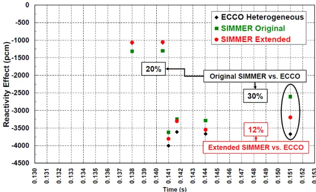
It is possible to note some of discrepancies from the degraded model 3 concerning the reactivity effects ( Figure 2.16) while heterogeneity effects and the value of k∞ are similar to values obtained by ECCO. The discrepancy in the reactivity effects is due to the different performance of the models; in ECCO finer energy groups are utilized.
22
Figure 2.15: Assessment of degraded fuel SA models.
Concluding, the SIMMER-III is applicable also in LWR, the results for not degraded conditions agree with reference, whereas in the degraded condition, efforts are going on to evaluate the effect of heterogeneity during an accidental scenario.
23
Figure 3.1: Overview of the MYRRHA FASTEF reactor and the SIMMER-III model.
The
Figure 3.1 also shows the representation created by SIMMER-III. A 2-Dimensional R-Z geometry was used, with a number of cells of 38x89. Only the fluid-dynamic model and the structure model were implemented in this calculation.
In Errore. L'origine riferimento non è stata trovata. the most important MYRRHA design parameters are summarized.
24
Table 3.1: MYRRHA design parameters.
General design parameters MYRRHA-FASTEF
Reactor power 100 MWth + 10 MWth
Maximum core inlet temperature 270 °C
Maximum core ΔT 140 °C
Average core outlet temperature 410 °C
Maximum hot plenum temperature 350 °C
Maximum fuel cladding temperature 466 °C
Pellet dimension Outside diameter: 5.42 mm
Fuel pin dimension Outside/Inside diameter: 6.55 mm/5.65 mm
Fuel pin length 1400 mm
Fuel active height 60 cm
Assembly type Hexagonal fuel bundle with wrapper with 127 pins
Assembly length 2000 mm
Maximum LBE bulk velocity 2 m/s
Core diameter and assembly 1450 mm and 151 position
Maximum core pressure drop 2.5 bar
3.1
Core modelling
In normal operation, at 100 MWth core power, the cold LBE (270°C) at high pressure flows through the assemblies installed in the core barrel. The fluid through the fuel assemblies (about 4926 kg/s) heats up to an average temperature of 410°C. The remaining LBE (about 4557 kg/s) flows through the reflector and dummy channels and other bypasses. The pressure drop over the core amounts to about 2.5 bar. Both LBE flows will mix in the hot plenum. An additional conservative heat up of 10 MW is considered due to additional heat sources such as the polonium decay, the heat dissipation of the pumps and the heat production in the in-vessel fuel storage. Accounting for this additional heating, the temperature of the hot plenum will reach 350°C. The temperature difference of 80°C between the hot plenum and the cold plenum is the maximal gradient allowed on the diaphragm to limit the thermal stresses on the component.
To obtain 100 MWth, a FASTEF critical core is necessary, illustrated in Figure 3.2.
Modelling the core by SIMMER-III, it is necessary to define the volume fractions of each component, so a FA architecture typical of SFR, described by Sarotto et al. in 2010 [8] was considered. In
Figure 3.3 is shown the FA architecture.
For simplicity and also because the neutronic model of SIMMER-III was not implemented in this modelling, an End Of Cycle (EOC) critical core was chosen (see Figure 3.4). Consequently, the absorber rods were not taken into account, in fact in this condition criticality is obtained with the 6 CR completely withdrawn. In the figure below is shown only the core region, except the dummy assemblies.
25
Figure 3.2: 100 MW - 69 FA critical core layout.
26
Figure 3.4: 100 MW - 69 FA EoC core layout (CR completely withdrawn).
The core was simulated by 8 rings, the first simulates the central IPS with the spallation target, the second, third and fourth rings simulate 15 FA each one, the fifth and sixth rings simulate 12 FA each one, the seventh ring simulates 24 inner dummies and the eighth ring simulates 42 Outer Dummies.
In the Figure 3.5 a comparison between the CAD and the SIMMER-III model is shown. The structure model was implemented to obtain the fuel pin and can wall configuration seen above.
27
Figure 3.6. Both the reactor cover and the reactor vessel are highlighted in red in the SIMMER-III modellization.
28
3.2.2 Diaphragm
The diaphragm is a mechanical structure composed by the main parts:
• lower plate with penetration for core support structure, in vessel fuel handling machine, in vessel fuel storages and primary pumps, recovery ports, LBE inlets, fuel transfer channels and wet-sipping devices; • upper plate with penetration for core support structure, in vessel fuel handling machines, primary
pumps, recovery ports, LBE inlets, fuel transfer channels and wet-sipping devices, primary heat exchangers, Si doping devices;
• casing and plates, they create a box for the primary pumps and primary heat exchangers and a box for the in vessel fuel storages, respectively.
The function of the diaphragm is to separate cold, high pressure LBE plenum, from hot, low pressure LBE plenum, to support and cool the In vessel fuel storage.
Figure 3.7 shows the comparison between the CAD model and the SIMMER-III model. The diaphragm representation in the code is highlighted in red in the SIMMER III nodalization (see
Figure 3.7).
29
30
3.2.4 Primary heat exchangers
The main thermal connection between the primary and the secondary system is provided by the Primary Heat Exchanger (PHX). In MYRRHA-FASTEF Reactor are provided 4 PHX with a power of 27.5 MW each.
In the
Figure 3.9, some details of the PHX represented by CAD and also by SIMMER-III are illustrated. Note that the PHX is highlighted in red.
In the present analysis, the PHX is simulated by a model performed by ENEA, using a heat sink to assure that the temperature in the outlet of the PHX is about 270°C.
31
32
4
STEADY-STATE RESULTS
The results of the performed analysis are reported below [9]. The steady-state conditions are reached in about 20 seconds, with value oscillations due to the code accuracy.
4.1
Temperature
Figure 4.1 shows the LBE temperature stratification predicted by the SIMMER-III code in steady-state conditions. The stratification occurs in the vessel upper plenum. This phenomenon requires more investigations because it causes temperature oscillations in the PHX inlet.
33
Figure 4.2: Temperature trends in cell [2,52] (middle of core).
Figure 4.3 shows the temperature axial profile in the active fuel zone in the second ring. A time of 100 seconds is chosen, in fact by this time steady-state conditions are already reached.
From this figure it can be noted that the LBE enters in the core with an average temperature of 269°C and exits with a temperature of 445°C, then, in the vessel’s upper plenum, the hot flow mixes with the cold flow of the outer ring and the temperature stabilizes at about 350°C. The max value of the clad, the pin surface and the center pin occurs above the middle of core.
34
Figure 4.3: Axially temperature profile in the active fuel zone in second ring.
The PHX in this simulation is represented with a proper heat sink to assure that the coolant inlet temperature in the core is 270°C. The dimension of the exchanger model is obtained by calculating the effective flow area of each PHX, so the equivalent area of the ring is the same value. The axial distance to the core, is the same as the design value because it is relevant in case of ULOF to maintain the natural circulation.
Figure 4.4 shows the temperature profile of the coolant in the PHX. As it is possible to note, the LBE enters in the exchanger with an average temperature of 357°C and exits with an average temperature of 269°C. It has to be noted that when stratification occurs, the inlet temperature of the coolant oscillates and this phenomena requires more investigations.
35
Figure 4.5: LBE velocity fields in steady-state conditions.
The velocity in PHX and in the core is reported in Figure 4.6. At steady-state conditions the value of velocity in the PHX is assessed in about 0.84 m/s, instead in the core at the inlet the velocity in the second ring is 0.80 m/s, and in the inner core is 1.70 m/s, below the technical limit of 2 m/s.
These results agree with the design values of 0.829 and 1.899 m/s, respectively for the LBE velocity in the PHX and in the core.
36
Figure 4.6: Velocity in the second ring at the inlet and inner of core and in the PHX.
4.3
Mass flow rate
Figure 4.7 shows trend mass flow rate in the primary heat exchanger and in the core. It is necessary to note that the value for the simulated PHX includes all 4 PHX actually presented. The mass flow rate in the PHX and in the core in steady-state is about 8770 kg/s, that is lower than the design value of 9480 kg/s because in this simulation, the mass flow rate in the gap wrapper is not taken into account, and also the IPS, the CR and the SR are not simulated. However, the mass flow rate simulated in the core region is about 4880 kg/s which is very close to the design value of 4926 kg/s.
37
38
5
TRANSIENT RESULTS
In order to assess the correct operability of the SIMMER-III modelling for fuel dispersion analysis in the primary circuit of the LBE-cooled MYRRHA reactor, some preliminary transient analyses have been initially performed under various plant operating conditions. Furthermore, some sensitivity calculations have been performed to investigate the influence of important parameters such as the fuel porosity on fuel distribution and accumulation in the primary circuit.
The present transient analysis is based on a preliminary 2D model of MYRRHA and is slightly different from the one described in the previous section 3. However, the general conclusions of these analyses are expected to apply also for the revised model to be used for more representative fuel dispersion studies.
5.1
Unprotected loss of flow transient
At first, an unprotected loss of flow (ULOF) transient has been simulated with SIMMER-III and the results have been compared with the results of the same transient analysed with the RELAP5 thermal-hydraulic code in the frame of the MYRRHA safety analysis.
This accidental transient is initiated by the loss of energy supply to both primary pumps without reactor scram, with consequent transition for forced to natural circulation in the primary circuit. The core power reduces due to negative reactivity feedbacks mainly induced by radial core and coolant expansion with increasing core temperatures. Since the neutronic model available in SIMMER-III is not applied in the present analysis, the core power evolution in the SIMMER-III calculation has been assigned as input data according to the transient value calculated by RELAP5 (see Figure 5.1).
Figure 5.1: Core nuclear power evolution in the ULOF transient,
The Figure 5.2 illustrates the LBE temperature and velocity fields in the primary circuit at t = 80 s from the beginning of the transient. The hot LBE flowing out from the active core rises to the LBE free level due to density effects and then flows through the upper holes of the core barrel within the upper plenum. In the upper plenum the hot LBE mixes with the colder LBE before reaching the IHX inlet and flowing back through the PHX-pump connecting compartment and the lower plenum towards the core inlet. The PHX, which
0.0 0.2 0.4 0.6 0.8 1.0 1.2 0 10 20 30 40 50 60 70 80 Time (s) R e la ti v e u n it Core power (R5) Core power (SIII)
39
Figure 5.2: LBE temperature and velocity field at t = 80 s in the ULOF transient.
The evolution of core mass flow rate predicted by SIMMER-III is compared with the RELAP5 calculated value in Figure 5.3. During the first 20 s, the core flow rate is mainly driven by the hot and cold LBE free levels equalization following primary pump coastdown. In fact, the pump speed halving time during coastdown (2 s) is small if compared to the time needed to reach stable LBE free levels. The minimum flow rate value is reached about 3 s earlier with SIMMER-III than with RELAP5. This deviation in code results is consistent with the different hot and cold LBE areas considered in the calculations, since the RELAP5 analysis was performed in a design configuration of MYRRHA, which is slightly different from the Version 1.2 of MYRRHA considered in the present analysis with SIMMER-III. After the initial transient phase with stabilization of natural circulation in the primary system in less than 30 s, the SIMMER-III code under-predicts the core flow rate with respect to RELAP5 by about 15%. This difference might be produced by the influence of enhanced thermal stratification and mixing effects that are predicted by SIMMER-III in the lower and upper plenum of the vessel, since these effects cannot be taken into account in the 1D simulation of the primary circuit with RELAP5.
40
Figure 5.3: Core mass flow rate evolution in the ULOF transient.
The Figure 5.4 shows the time evolution of the maximum clad temperature calculated by the two codes. The small deviation observed between SIMMER-III and RELAP5 results is consistent with the discrepancy observed in the core mass flow rate evolution in Figure 5.3. Since all the fuel assemblies have the same mass flow rate, the maximum clad temperature is exhibited in the first core ring where the neutronic power reaches its maximum value. After a noticeable peak in the clad temperature that rises to about 1050-1100 °C in the first 15–20 s, the maximum clad temperature reduces and then stabilizes around 760-800°C. Because of the reduced core flow rate, the temperature predicted by SIMMER-III is greater than the RELAP5 by about 40°C.
In conclusion, the ULOF transient analysis with SIMMER-III and the successful comparison with RELAP5 results confirm the ability of the code to simulate transient conditions in LBE-cooled systems, despite the necessary simplifications introduced in the 2D SIMMER-III modelling for simulating the complex 3D geometry of the primary system of MYRRHA.
0.0 0.2 0.4 0.6 0.8 1.0 1.2 0 10 20 30 40 50 60 70 80 Time (s) R e la ti v e u n it Core flow (R5) Core flow (SIII)
41
Figure 5.4: Maximum clad temperature evolution in the ULOF transient.
5.2
Fuel dispersion analysis
Under accidental conditions, the release of fuel to the coolant can occur in case of fuel rod clad failure and degradation. In a LBE-cooled reactor like MYRRHA, the stainless steel clad material has a melting point lower than the boiling point of LBE, therefore, clad melting and consequent fuel dislocation is expected before coolant boiling, with consequent release of solid fuel fragments (chunk or particles) in the flowing LBE.
Another important aspect to be taken into account for fuel dispersion in the coolant is the relative density of the fuel (MOX with 30% of plutonium) and the LBE. In fact, the MOX density is very close to the coolant density, as indicated in Figure 5.5. While the coolant density depends almost exclusively on temperature, the fuel density may depend not only on temperature, but also on the degree of porosity, which reduces the fuel density with respect to the theoretical value. On its turn the fuel porosity depends on fuel swelling under irradiation conditions and, thus the porosity increases from the initial value, usually close to 5%, up to about 10% towards the end of the irradiation cycle inside the reactor.
Figure 5.5 shows that, depending on the degree of fuel porosity, the MOX density can be higher or lower than the LBE density in the normal operating temperature range of the MYRRHA reactor between 270–350°C. How the fuel porosity can influence the fuel distribution and accumulation in the primary circuit is one of the main aspects investigated in the present analysis.
400 500 600 700 0 10 20 30 40 50 60 70 80 Time (s) T e m p
42
Figure 5.5: Density versus temperature for LBE and MOX with different porosity.
Because of the small density difference between fuel and coolant, the drag forces can prevail on buoyancy forces according to the influence of coolant velocity and flow pattern in different zones of the primary system. For this reason the fuel dispersion in the primary circuit has been investigated under both forced circulation at nominal power and natural circulation conditions, following reactor scram and primary pump coastdown.
In the present analysis, no reference to specific accidental transient is made to determine the conditions for fuel release to the coolant from affected fuel rods, but, arbitrarily, the release of a certain amount of fuel, equivalent to 1 fuel rod, is assumed in the inner ring of the core. The fuel is released to coolant as particles with size of 1 mm in diameter (default value of SIMMER-III code).
5.2.1 Forced circulation in the primary circuit
The fuel release from the core and its distribution in the primary circuit is evaluated with the reactor at full power (110 MWth) and with primary pumps at nominal speed. Two calculations have been performed using fuel with different degree of porosity. In the first calculation the fuel porosity is assumed equal to 5%. The redistribution of fuel and its accumulation in the primary circuit calculated by SIMMER-III is illustrated in Figure 5.6 which shows the fuel particle concentration in the coolant at different instants during the transient phase. Once the fuel is released to the flowing LBE inside the core, the coolant transports the fuel particles out of the core and towards the top of the upper plenum.
9700 9800 9900 10000 10100 10200 10300 10400 10500 10600 200 250 300 350 400 450 500 550 600 Temperature (°C) D e n s it y ( k g /m 3 ) MOX (p = 5%) MOX (p = 6%) MOX (p = 7%) MOX (p = 8%) MOX (p = 9%) MOX (p = 10%) LBE T lower plenum T upper plenum
43
Time = 90 s Time = 180 s Time = 300 s
Figure 5.6: Evolution of fuel particle concentration in the primary circuit (fuel porosity = 5%).
The fuel particles then move radially, through the core barrel holes, towards the external part of the upper plenum. As the fuel particles distribute within the upper plenum, their concentration progressively reduces. Because of the low density difference between the coolant and the fuel, the drag forces induced by the flowing coolant still prevails on buoyancy effects and thus a noticeable amount of fuel particles are transported to the PHX inlet. From the PHX outlet, the fuel particles enter the PHX-pump connecting compartment where large coolant mixing and recirculation take place. The primary pump pushes the fuel particles still trapped inside the coolant towards the bottom part of the lower plenum, where, once more, enhanced coolant mixing takes place.
Inside the lower plenum the fuel particles partly move towards the core inlet following the main coolant flow path, and partly tend to settle down onto the bottom surface of the vessel, in the more stagnant region of the lower plenum, because of the slightly higher density of the fuel with respect to the coolant at 270°C (lower plenum temperature).
44
The fuel particles that reach the core inlet, after about 60 s from the beginning of the transient, are almost uniformly distributed inside the core and leave the core at the outlet to start a new round within the primary circuit.
After 300 s from transient initiation, the fuel distribution and accumulation in the primary system is characterized by a large spreading of fuel particles over the entire primary volume with a very low fuel particle concentration value. Larger fuel particle concentrations are exhibited in specific regions of the primary circuit in which the coolant becomes almost stagnant and where buoyancy forces can prevail on drag forces. The maximum concentration of particles seems reached at the vessel bottom where the coolant velocity pattern indicates that an almost stagnant region develops. Some smaller accumulation of fuel particles is also exhibited inside the PHX-pump connecting compartment, particularly inside the corner regions where coolant flow is limited. Some fuel particles tend to settle down due to gravity effect onto the diaphragm upper plate. However, coolant flow recirculation inside the upper plenum may cause the re-suspension of these particles, thus limiting the accumulation effect.
In order to evaluate the influence of coolant-fuel density difference on fuel distribution and accumulation in the primary circuit, a second calculation has been performed with fuel porosity equal to 10%. In this case the fuel is slightly denser than the coolant over the full primary temperature range.
The evolution of fuel particle redistribution and accumulation in the primary circuit calculated by SIMMER-III is illustrated in
Figure 5.7. Since the transport of fuel particles is mainly driven by the moving coolant and induced drag forces, the trajectory of particles within the primary circuit is similar in the two cases with different porosity. However, the buoyancy effects, even if they are smaller comparing to the drag effects, may produce some significant difference in the overall distribution of fuel particles within the primary circuit, as
highlighted by the evolution of fuel dispersion shown in Figure 5.7 in comparison to Figure 5.6.
With the highest porosity, the fuel particles tend to preferentially accumulate and float at the LBE free surface of the upper plenum, as evidenced at t =300 s in
Figure 5.7. Furthermore, fuel particles transported in the lower plenum might move slowly upwards until they are stopped by the lower plate of the diaphragm structure. Some of these particles rise up in the almost stagnant annular space between the diaphragm and the cylindrical vessel wall, which also includes the volume occupied by the fuel handling channels in the 2D SIMMER-III simulation of the primary system. Figure 5.8, which shows the fuel particle concentration in the primary circuit after 2700 s from transient initiation, highlights the fuel particle accumulation occurring at the LBE free surface in the long term. Mainly due to fluctuations at the free surface and mixing in the upper plenum, some of the fuel particles are trapped in the moving coolant and continue to circulate in the primary circuit. Other less important points of accumulation are the downward surface of the diaphragm lower plate and the upper volume of the PHX-pump connecting compartment.
45
Time = 90 s Time = 180 s Time = 300 s
46
Figure 5.8: Fuel particle concentration in the primary circuit at t = 2700 s (fuel porosity = 10%).
5.2.2 Natural circulation in the primary circuit
In this transient analysis, primary pump coastdown and reactor scram and are initiated 10 s after the beginning of the transient phase releasing fuel particles from the core. As a consequence, the core nuclear power reduces to the decay level and natural circulation tends to stabilize in the primary circuit.
Both calculations with low (5%) and high (10%) fuel porosity have been performed in order to investigate the influence of buoyancy effect in a situation in which the drag force is much less important than in the previous case with forced circulation in the primary circuit.
Figure 5.9 illustrates the fuel particle concentration calculated by SIMMER-III at t = 300 s in case of low fuel porosity value. Before primary pump coastdown initiation at t = 10 s, most of the fuel particles are transported by the coolant, through the core barrel, inside the upper plenum. After primary pump coastdown at t = 10 s, the coolant flows in the primary circuit are mainly driven by the LBE hot and cold free
level equalization, as already discussed in section 5.1 in case of ULOF transient. As a consequence, the coolant flow reverses inside the PHX thus limiting the transport of fuel particles through the PHX-pump connecting compartment towards the lower plenum. Therefore, most of the fuel particles remain confined inside the upper plenum, also because of the limited drag forces related to natural convective movements.
As clearly indicated in
Figure 5.9, the buoyancy effect seems to prevail on the drag force inside the upper plenum and the fuel particles tend to settle down and distribute onto the upward surface of the diaphragm upper plate. Similarly, the fuel particles that reached the PHX-pump connecting compartment are expected to mainly accumulate in the lower part of this volume in the following phase of the transient.
47
Figure 5.9: Fuel particle concentration in the primary circuit at t = 300 s (fuel porosity = 5%).
The situation regarding fuel dispersion is clearly different from the previous one in the case of high porosity fuel particles as shown in
Figure 5.10. The evolution of the thermal-hydraulic transient is the same since the small amount of fuel release considered cannot produce any deviation in the overall system. However, due to the opposite density difference (in this case the fuel is slightly lighter than the coolant) the fuel particles inside the upper plenum tend to accumulate and float on the LBE free surface. For the same reason, the fuel particles that reached the PHX-pump connecting compartment accumulate in the uppermost part of the volume.
48
49
conjunction with the flow regime and respective coolant velocity pattern which stabilized in the primary circuit, seems to have a significant influence on fuel accumulation and redistribution. For low porosity values the fuel particles tend to settle down onto lowest surfaces, while for high porosity values the fuel particles tend to float at the LBE free surface. This qualitative fuel particle behaviour has to be confirmed with the use of the revised 2D model of MYRRHA and by more detailed 3D simulations with SIMMER-IV code.
50
REFERENCES
[1] AA.VV., “SIMMER III Structure model: model and method description”, Research Document, O-arai Engineering Center, Japan Nuclear Cycle Development Institute, JNC TN 9400 2004-043.
[2] Morita K., et al., “SIMMER-III applications to fuel-coolant interactions”, Nucl.Eng.Des. 189 (1999) 337-357.
[3] Tobita Y., et al., “Evaluation in a CDA Energetics in the Prototype LMFBR with Latest Knowledge and Tools”, Proc.7th Int. Conf. Nuclear Engineering, (ICONE 7), Tokio, Japan, 12-23 April 1999.
[4] Liu P., et al., “Transient analyses of the 400MWth-class EFIT accelerator driven transmuter with the multi-physics code: SIMMER-III”, Nucl.Eng.Des. 240 (2010) 3481-3494.
[5] Yamano H., et al., “A three-dimensional neutronics-thermohydraulics simulation of core disruptive accident in sodium-cooled fast reactor”, Nucl.Eng.Des. 239 (2009) 1673-1681.
[6] Wang S., et al., “Molten salt related extensions of the SIMMER-III code and its application for a burner reactor”, Nucl.Eng.Des. 236 (2006) 1580-1588.
[7] Gabrielli F., et al., “Extensions of the SIMMER Code for Sever Accident Analyses in Light Water Reactor”, 16th SIMMER-III/IV Review Meeting, University of Pisa, 29th May – 1st June 2012.
[8] AA.VV., “Critical FASTEF ‘frozen’ design configuration for thermal-hydraulic safety studies within CDT Task 2.3”, EU-FP7 CDT Project, REP006-2011, May 2011.
[9] AA.VV., “SIMMER III input manual”, Research Document, O-arai Engineering Center, Japan Nuclear Cycle Development Institute, 2003.
51
α volume fraction
δ length [m]
κ thermal conductivity [W/(m K)]
ρ density [kg/m3]
τ structure time constant [s]
Abbreviations and acronyms
ADS Accelerator Driven System AFDM Advanced Fluid-Dynamics Model
BT Beam Trip
CAD Computer Aided Design CDA Core Disruptive Accident
CEA Commissariat à l'Énergie Atomique
CR Control Rod
EoC End of Cycle
EOS Equation of State
FA Fuel Assembly
FCI Fuel Coolant Interaction
FP Fission Product
FZK Forschungszentrum Karlsruhe IPS In Pile Section
JNC Japan Nuclear Cycle Development Institute LANL Los Alamos National Laboratory
LBE Lead Bismuth Eutectic LFR Lead Fast Reactor
LMFR Liquid Metal Fast Reactor
MOSART MOlten SAlt Advanced Reactor Transmuter
52 MSBR Molten Salt Breeder Reactor
MSRE Molten Salt Reactor Experiment NPSH Net Positive Suction Head PBA Protected Blockage Accident PHX Primary Heat Exchanger PLOF Protected Loss Of Flow
PNC Power Reactor and Nuclear Fuel Development Corporation PTOP Protected Transient OverPower
RIA Reactivity Induced Accident
SA Sub Assembly
SFR Sodium Fast Reactor
SR Safety Rod
UBA Unprotected Blockage Accident ULOF Unprotected Loss Of Flow
UTOP Unprotected Transient OverPower
53
Ha conseguito la laurea triennale in Ingegneria Energetica nel 2009 e successivamente la laurea specialistica in Ingegneria Energetica nel 2011 presso l'Università di Pisa. Nel lavoro di tesi specialistica ha analizzato il fenomeno dello "sloshing" e dell'interazione fluido-struttura con riferimento ai reattori di IV Generazione refrigerati a metallo liquido soggetti a sollecitazioni dinamiche esterne (ad esempio un sisma). Da gennaio 2012 è borsista presso il DIMNP dell'Università di Pisa.
Nicola Forgione
Ricercatore in Impianti Nucleari presso il Dipartimento di Ingegneria Meccanica, Nucleare e della Produzione (DIMNP) dell’Università di Pisa dal 20 dicembre 2007. Laureato in Ingegneria Nucleare nel 1996 presso l’Università di Pisa ed in possesso del titolo di Dottore di Ricerca in Sicurezza degli Impianti Nucleari conseguito all’Università di Pisa nel 2000. La sua attività di ricerca è incentrata principalmente sulla termofluidodinamica degli impianti nucleari innovativi, con particolare riguardo ai reattori nucleari di quarta generazione. Autore di oltre 20 articoli su rivista internazionale e di numerosi articoli a conferenze internazionali.