Dipartimento di Informatica
Dottorato di Ricerca in Informatica XII Ciclo - Nuova Serie
Tesi di Dottorato in
New Methods, Techniques and
Applications for Sketch Recognition
Mattia De Rosa
Ph.D. Program Chair Supervisors
Prof. Giuseppe Persiano Prof. Gennaro Costagliola
Dott. Vittorio Fuccella
Abstract
The use of diagrams is common in various disciplines. Typical examples include maps, line graphs, bar charts, engineering blueprints, architects’ sketches, hand drawn schematics, etc.. In general, diagrams can be created either by using pen and paper, or by using specific computer programs. These programs provide functions to facilitate the creation of the diagram, such as copy-and-paste, but the classic WIMP interfaces they use are unnatural when compared to pen and paper. Indeed, it is not rare that a designer prefers to use pen and paper at the beginning of the design, and then transfer the diagram to the computer later.
To avoid this double step, a solution is to allow users to sketch directly on the computer. This requires both specific hardware and sketch recognition based software. As regards hardware, many pen/touch based devices such as tablets, smartphones, interactive boards and tables, etc. are available today, also at reasonable costs. Sketch recognition is needed when the sketch must be processed and not considered as a simple image and it is crucial to the success of this new modality of interaction. It is a difficult problem due to the inherent imprecision and ambiguity of a freehand drawing and to the many domains of applications. The aim of this thesis is to propose new methods and applications regarding the sketch recognition. The presentation of the results is divided into several contributions, facing problems such as corner detection, sketched symbol recognition and autocompletion, graphical context detection, sketched Euler diagram interpretation.
The first contribution regards the problem of detecting the corners present in a stroke. Corner detection is often performed during preprocessing to segment a stroke in single simple geometric primitives such as lines or curves.
The corner recognizer proposed in this thesis, RankFrag, is inspired by the method proposed by Ouyang and Davis in 2011 and improves the accuracy percentages compared to other methods recently proposed in the literature. The second contribution is a new method to recognize multi-stroke hand drawn symbols, which is invariant with respect to scaling and supports symbol recognition independently from the number and order of strokes. The method is an adaptation of the algorithm proposed by Belongie et al. in 2002 to the case of sketched images. This is achieved by using stroke related information. The method has been evaluated on a set of more than 100 symbols from the Military Course of Action domain and the results show that the new recognizer outperforms the original one.
The third contribution is a new method for recognizing multi-stroke par-tially hand drawn symbols which is invariant with respect to scale, and supports symbol recognition independently from the number and order of strokes. The recognition technique is based on subgraph isomorphism and exploits a novel spatial descriptor, based on polar histograms, to represent relations between two stroke primitives. The tests show that the approach gives a satisfactory recognition rate with partially drawn symbols, also with a very low level of drawing completion, and outperforms the existing ap-proaches proposed in the literature. Furthermore, as an application, a system presenting a user interface to draw symbols and implementing the proposed autocompletion approach has been developed. Moreover a user study aimed at evaluating the human performance in hand drawn symbol autocompletion has been presented. Using the set of symbols from the Military Course of Action domain, the user study evaluates the conditions under which the users are willing to exploit the autocompletion functionality and those under which they can use it efficiently. The results show that the autocompletion functionality can be used in a profitable way, with a drawing time saving of about 18%.
The fourth contribution regards the detection of the graphical context of hand drawn symbols, and in particular, the development of an approach for identifying attachment areas on sketched symbols. In the field of syntactic recognition of hand drawn visual languages, the recognition of the relations
among graphical symbols is one of the first important tasks to be accomplished and is usually reduced to recognize the attachment areas of each symbol and the relations among them. The approach is independent from the method used to recognize symbols and assumes that the symbol has already been recognized. The approach is evaluated through a user study aimed at comparing the attachment areas detected by the system to those devised by the users. The results show that the system can identify attachment areas with a reasonable accuracy.
The last contribution is EulerSketch, an interactive system for the sketching and interpretation of Euler diagrams (EDs). The interpretation of a hand drawn ED produces two types of text encodings of the ED topology called static code and ordered Gauss paragraph (OGP) code, and a further encoding of its regions. Given the topology of an ED expressed through static or OGP code, EulerSketch automatically generates a new topologically equivalent ED in its graphical representation.
I would like to thank my advisor Gennaro Costagliola and Vittorio Fuccella, who coauthored most of the papers related to this thesis, for the profitable discussions that contributed to my research work and for the suggestions and help they gave me during the preparation of this thesis. I also thank Vittorio Fortino for the contribution on the development of RankFrag and Paolo Bottoni, Andrew Fish and Rafiq Saleh, who have been co-authors for recent research papers on Euler diagrams related to the results presented in this thesis.
Contents
Abstract i
Acknowledgement iv
Contents iv
1 Introduction 1
1.1 Key aspects of sketch recognition . . . 3
1.2 Proposed work . . . 5
1.3 Outline . . . 8
2 Related Work 10 2.1 Corner detection . . . 10
2.2 Sketched symbol recognition . . . 12
2.3 Autocompletion . . . 14
2.4 Attachment areas . . . 16
2.5 Euler diagram sketching . . . 17
3 RankFrag: a Novel Technique for Corner Detection in Hand Drawn Sketches 18 3.1 The RankFrag technique . . . 19
3.1.1 Complexity . . . 23 3.1.2 Features . . . 24 3.1.3 Classification method . . . 27 3.1.4 Implementation . . . 28 3.2 Evaluation . . . 28 v
3.2.1 Model validation . . . 28
3.2.2 Accuracy metrics . . . 30
3.2.3 Data sets . . . 30
3.3 Results . . . 31
3.4 Concluding remarks . . . 32
4 Improving Shape Context Matching for the Recognition of Sketched Symbols 34 4.1 Background: symbol recognition through shape context . . . . 35
4.1.1 Feature descriptor . . . 35 4.1.2 Matching . . . 37 4.2 The approach . . . 37 4.2.1 An example . . . 38 4.3 Evaluation . . . 39 4.4 Concluding remarks . . . 40
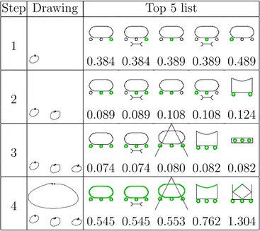
5 Recognition and Autocompletion of Partially Drawn Sym-bols by Using Polar Histograms as Spatial Relation Descrip-tors 41 5.1 Recognition of partially drawn symbols . . . 43
5.1.1 Symbol pre-processing . . . 43
5.1.2 PSR descriptor . . . 45
5.1.3 Symbol representation . . . 46
5.1.4 Symbol matching . . . 47
5.2 An interactive system for the autocompletion of hand drawn symbols . . . 58
5.2.1 Back-end . . . 59
5.3 Evaluation . . . 61
5.3.1 Data sets . . . 62
5.3.2 Performance of the recognizer . . . 63
5.3.3 Performance of the PSR descriptor . . . 67
5.3.4 Performance of the interactive system . . . 69
5.4.1 Completion times . . . 71
5.4.2 Menu use . . . 73
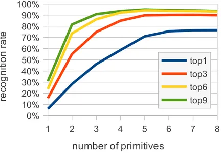
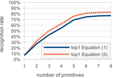
5.4.3 Analysis by the number of primitives . . . 73
5.4.4 Accuracy . . . 75
5.4.5 Comments from the participants . . . 76
5.5 Concluding remarks . . . 76
6 Identifying Attachment Areas on Sketched Symbols 79 6.1 The approach . . . 80 6.1.1 Symbol representation . . . 81 6.1.2 Point matching . . . 83 6.1.3 Area identification . . . 84 6.2 Evaluation . . . 85 6.2.1 Results . . . 87 6.3 Concluding remarks . . . 89
7 EulerSketch: a sketch system for Euler diagrams 91 7.1 Static code and ordered Gauss paragraph . . . 92
7.2 User interface . . . 94
7.3 Back-end . . . 97
7.4 Concluding remarks . . . 98
8 Achievements and Future Research 99 A Data sets 102 A.1 IStraw . . . 103 A.2 NicIcon . . . 103 A.3 Composite . . . 103 A.4 COAD . . . 105 A.5 COAD2 . . . 106 Bibliography 108
Introduction
The use of diagrams is common in various disciplines. The term can have different meanings depending on the context, and in fact, there is no single definition of diagram in the scientific literature. In general, a diagram can be defined as a visual representation of some information and it is usually two-dimensional and geometric. Under this definition, typical examples of diagrams include maps, line graphs, bar charts, engineering blueprints, architects’ sketches, hand drawn schematics, etc.. Diagrams are often used to represent the information in a natural way. It is generally easier, faster and more convenient to grasp the meaning of a visual representation than the meaning of a textual representation. In some cases the use of diagrams is practically inevitable, given that an equivalent textual representation would be too long and complex (for example in the case of architectural plan, etc.). The notion that a complex idea can be conveyed with just a single still image is common knowledge, as in the adage “A picture is worth a thousand words”.
In general, diagrams can be created either by using pen and paper, or by using specific computer programs. With the introduction of the mouse, these programs have started to use the same paradigm, in which the use of a palette allows to select and place individual elements of the diagram on a canvas. These programs provide functions to facilitate the creation of the diagram, such as copy-and-paste, automatic layout and much more. However, the interfaces of these programs are still unnatural when compared to pen
and paper, and the way they work is often dictated by technical limitations rather than by the needs of the users.
Indeed, it is not rare that a designer prefers to use pen and paper at the beginning of the design, and then transfer the diagram to the computer later when the idea has taken its almost final shape. For many people, pen and paper are easier and faster to use, they are also more flexible (because paper does not have an explicit interface) and promote increased creativity, supporting also activities in which the vagueness of the result is an essential feature. Also, informal sketching can be convenient in the context of group work.
The effort necessary for the creation of informal sketches is typically much lower than that for the creation of more precise, formal diagrams with mouse and palette, even though it requires an additional effort for subsequently transferring the sketches to the computer. To solve this drawback, one possibility is therefore to allow users to sketch directly on the computer. In this case, specific hardware for drawing is necessary, such as pen tablets and touch screens. This hardware has become very popular in recent years in the form of drawing boards, tablets and smartphones which allow the use of pens, fingers, or both.
The use of these types of input devices enables a paradigm of communica-tion with the computer completely different from that of the classical WIMP (window, icon, menu, pointing device) user interfaces. Of course to better
exploit this new paradigm, dedicated software needs to be used.
This new paradigm allows to study the possibility of putting together the best features of the two types of interaction: a very simple and natural interface such as pen and paper, and the functions only possible with a computer program such as copy and paste, multiple saves, etc. In this context, the possibility arises to allow the user to draw a sketch directly on the computer, and then, through a recognition operation, automatically convert it into a more formal form, equivalent to that which can be produced with a classical WIMP interface. This operation is realized through techniques of sketch recognition, and marks the difference from a simple drawing program. The use of sketch recognition techniques allows, among other things, to
provide additional functionalities in software systems, such as real time help, more powerful editing, autocompletion, beautification, automatic layout (to remove clutter and confusion), interpretation and translation of the sketch.
Sketching recognition is also used to resolve problems created by the re-placement of paper and pen with WIMP systems. As an example, customers (e.g. of an architect) may be reluctant to criticize drawings that look too “finished”. Given that low-fidelity sketches do not have this problem, it is possible to show them to the customers and then use sketch recognition capa-bilities to produce the “finished” version of the drawing (without additional work).
On the other hand, sketch recognition is a difficult problem due to the inherent imprecision and ambiguity of a freehand drawing. Because of this, the problem of sketch recognition is usually divided into multiple specific “easier” problems. Often the methods used to solve these individual problems are not tied exclusively to the sketch recognition and are also used in other domains.
The next section will describe the main aspects of the sketch recognition, while Section 1.2 will briefly describe the new methodologies proposed in this thesis, which will then be discussed in detail in later chapters.
1.1
Key aspects of sketch recognition
This section discusses the general terms and definitions in the field of sketch recognition.
A central element of sketching is the stroke. On a touch screen, a stroke starts with the pressure of the pen (or finger) on the screen and ends when the pen is raised. Technically, a stroke is a finite list of triples (x, y, t) (or samples) where (x, y) are the pair of coordinates in which the pen was at the time t. Is possible to extend this definition by adding the pressure applied on the screen (if the hardware can detect it), therefore a stroke becomes a list of quadruples (x, y, t, p). This value can be used to improve the accuracy of the recognition process, or only to vary the thickness of the displayed stroke.
the recognition, or rather the recognition of the individual symbols that compose a sketch starting from the individual strokes. A symbol can be considered one of the basic blocks that constitute a sketch in a given domain. Of course, in order to identify individual symbols, they must be included in the definition of the given domain. Sometimes a drawing can also include text to add additional information.
Sometimes the recognition is divided into two levels, low-level recognition (or preprocessing) and high-level recognition. In this case the first step is used to extract intermediate information from the strokes, while the second uses this information to recognize the symbols.
As already pointed out, recognition is a difficult problem, both because hand-drawing can be imprecise and ambiguous, and also because there is a lot of variability in the drawing of different people and it is not uncommon to see significant variations even by the same person.
After the identification of the individual symbols the next step is under-standing the sketch as a whole. This phase depends greatly on the approach and on the domain. For example, it is possible to analyze the relationships between the different symbols in order to obtain meaningful information.
The various approaches for the recognition vary in the characteristics required in the input. The simplest approaches require that each stroke corresponds to a single symbol, thus simplifying the recognition. To remove this requirement it is necessary to solve two types of problems (often associated with the preprocessing): the clustering in which different strokes must be put together to represent a symbol, and the segmentation in which a stroke must be divided if it contributes to more than one symbol. In some cases, these steps can be used to group/split individual strokes in order to get simple geometric primitives (such as a line or a curve), instead of the whole symbol. The first type of approach is called single-stroke, while the second multi-stroke. Technically, when the recognition is performed from strokes, it is called online, when it is performed from a raster image it is called off-line. In addition, if the recognition can begin after (or even during) the input of each stroke, it is called eager recognition, while if it begins after the drawing is complete it is called lazy recognition. Eager recognition may be associated
with autocompletion and with the ability to provide immediate feedback to the user, even before s/he has finished the drawing. In this case, the recognition needs to be fast enough to allow a fluid interaction with the user.
As regards the design of sketch-based user interfaces, there is a need of distinguishing drawing strokes from editing commands. For example, a user interface may allow the deletion of a symbol by drawing a cross above it. This introduces further ambiguity, as it becomes necessary to determine whether a stroke is part of the input drawing or represents an editing command. To avoid this ambiguity, it is possible to use approaches in which the user must change the input mode depending on the operation that s/he intends to perform (for example, by clicking on a softbutton “pen” to insert a stroke or a softbutton “rubber” to erase). The latter approach is called “mode-based”, while the former “mode-less”. Generally, modes are to be avoided, even though they simplify recognition. For example, in the case of handwriting input it is possible to use both approaches, but the mode-less writing adds the difficulty of distinguishing between text and drawings, which is still an open issue.
1.2
Proposed work
The aim of this thesis is to propose new methods and applications regarding the sketch recognition by facing problems such as corner detection, sketched symbol recognition and autocompletion, graphical context detection, sketched euler diagram interpretation. The methodologies presented can be used as intermediate steps in the broader problem of the recognition of an entire diagram, and for this reason are logically linked to each other.
A first contribution regards the detection of the corners present in a stroke. Corner detection is often performed during the phase of preprocessing to segment a stroke into single simple geometric primitives such as lines or curves. The so obtained segments can then be used as input for a sketch recognition algorithm. The corner recognizer proposed in this thesis, RankFrag, is inspired by the method proposed by Ouyang and Davis in [1] and improves the accuracy percentages compared to other methods recently proposed in the literature.
The second contribution regards the recognition of multi-stroke hand drawn symbols. Symbol recognition is one of the main “basic” issues in the context of sketched diagram recognition. In fact, when an entire diagram is to be recognized, it is usually necessary to proceed with the recognition of the individual symbols composing it and of the connectors among them. The proposed method is an adaptation of the image-based matching algorithm by Belongie et al. [2]. As the original algorithm, the proposed solution is invariant with respect to scaling and is independent from the number and order of the drawn strokes. Furthermore, it has a better recognition accuracy than the original one when applied to hand drawn symbols as resulting from the evaluation of the method on a set of more than 100 symbols belonging to the Military Course of Action domain. This is due to the exploitation of information on stroke points, such as the temporal sequence and occurrence information in a given stroke.
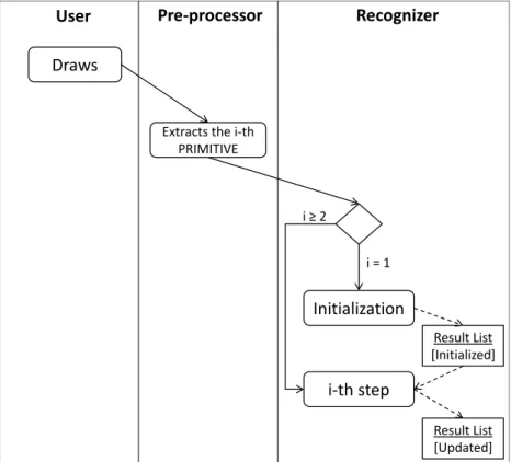
The third contribution regards the recognition of partially drawn symbols. The proposed method is invariant with respect to scale and uses an Attributed Relational Graph (ARG) [3] to represent symbols. Furthermore, the user can draw a symbol with the desired number of strokes and in any order. The method works with a single perfect template for each class, without the need of a training phase to extract features or to select multiple templates. Being based on subgraph matching, the recognition can be performed on partially drawn symbols, i.e., when only a part of the primitives composing the symbol is available. An innovation of the presented method is the use of a single spatial descriptor to represent relations between symbol components. The descriptor is an adaptation of the shape context [2] and its use makes the method free from the identification of the type of the primitives and from the check of fuzzy relations. The symbol matching is performed through an approximate graph matching procedure which incrementally produces new results as soon as more input strokes are available. Furthermore, a system presenting a user interface to draw symbols and implementing the proposed autocompletion method has been developed. Since autocompletion has proven to be an effective and appreciated feature when considering text editing applications [4, 5, 6, 7] but there are no evaluations of the performance of interfaces for autocompletion
of hand drawn symbols in the scientific literature, the system has been used to test the hand drawn symbol autocompletion functionality from the point of view of the benefits for the users. The user study has involved 14 participants and has shown that the users can exploit the autocompletion functionality in a profitable way, obtaining a faster input, with a time saving of about 18% and an increased accuracy.
The fourth contribution regards graphical context detection, and in particu-lar, the identification of the attachment areas on sketched symbols. According to a largely accepted model in the visual language community the relations be-tween the symbols of a diagram are geometrically defined through attachment areas of the symbols. For example, an arc of a graph is entering a node if the head of the arc is physically connected to the node boundary. Here, the rela-tion entering between arc and node is defined on the attachment area head of the arc and the attachment area boundary of the node. Attachment areas can have different shapes and are generally related to the physical appearance of the symbol. In WIMP-based systems, the attachment areas are automatically reported by the system. In a sketched language, due to the impreciseness of hand-drawing, actual attachment areas of symbols may be heavily deformed [8]. The management of areas which are not delimited by the visible ink of the drawn symbol can be even more difficult. The proposed approach is independent from the domain of the symbols and from the method used to recognize symbols and assumes that the symbol has already been recognized. This also means that the ink drawn by the user to sketch the symbol has already been separated from the other ink in the diagram. The approach requires that the symbol and, more precisely, both its physical and logical features, are defined in vector graphics. The identification of the attachment areas is performed by establishing a mapping between sampled points of both the sketched and the template symbol. The approach is evaluated through a user study in which users are required to sketch symbols from different domains and then to identify attachment areas on the drawn symbol.
Finally, the last contribution regards the development of EulerSketch, an interactive system for the sketching and interpretation of Euler diagrams (EDs). EDs are used for visualizing relationships between set-based data [9].
They consist of a set of curves representing sets and their relationships. EDs are, as example, utilized in various information presentation applications as a simple, yet effective means of representing and interacting with set-based relationships. Given the simplicity of EDs, it was not necessary to use the sketch recognition techniques proposed so far in EulerSketch. Nevertheless, EulerSketch it is still an interesting prototype in that it shows a concrete example of the possibilities given by the interpretation and translation of sketches. In fact, EulerSketch allows to sketch Euler diagrams, and its main feature is the possibility of transforming a drawn ED into two types of text encodings of the ED topology called static code and ordered Gauss paragraph (OGP). In addition to classic editing operations, such as delete and move, the system allows the visualization of the static code and of the OGP of the drawn diagram and the corresponding encoding of its regions. Moreover, given the topology of an ED expressed through static code or OGP, it also allows to automatically generate a new topologically equivalent ED in its graphical representation. This functionality can be used both to display a new diagram from an edited code and to generate alternative and equivalents views of a sketched ED.
As mentioned at the beginning of this section, there are logical links between the various proposed methods. The most important is the one between RankFrag and the approach for the recognition of partially drawn symbols. As a matter of fact, RankFrag is the corner detection algorithm used for the segmentation of strokes as part of the preprocessing of the autocompletion system. As regards the approach for identifying attachment areas on sketched symbols, since it takes for granted the recognition of the symbol, it is therefore possible to integrate it with one of the proposed recognition methods.
1.3
Outline
In this thesis, each chapter is devoted to the contribution to a single area of the sketch recognition. Chapter 2 describes the related works; Chapter 3 describes RankFrag, the method for corner recognition; Chapter 4 describes
the approach for the recognition of multi-stroke hand drawn symbols1; Chapter
5 describes the approach for the recognition of partially drawn symbols and the evaluating the human performance in hand drawn symbol autocompletion2;
Chapter 6 describes the approach for identifying attachment areas on sketched symbols3; Chapter 7 describes EulerSketch, the system for the sketching of
Euler diagrams4; Chapter 8 presents some final remarks and a brief discussion
on future works. Finally, Appendix A shows the data set used to test the proposed methods.
1The content of Chapter 4 is based on the following peer-reviewed paper: [10]
2The content of Chapter 5 is based on the following peer-reviewed papers: [11], [12],
[13].
3The content of Chapter 6 is based on the following peer-reviewed paper: [14]. 4The content of Chapter 7 is based on the following peer-reviewed papers: [15], [16].
Chapter 2
Related Work
This section describes the related work regarding the sketch recognition aspects treated in this thesis, devoting a section to each of them.
2.1
Corner detection
Corner detection is a fundamental component in creating sketch recognizers. Since corners represent the most noticeable discontinuity in the graphical strokes, their detection is often used in the segmentation (or fragmentation) of input strokes into primitives.
Important features for corner detection techniques include the high pre-cision, the possibility to be performed in real time, and the capacity of adaptation to user preferences, to user drawing style and to the particular application domain. The adaptation to the domain can be achieved by using techniques based on machine learning. Almost all of the most recent methods use machine learning techniques, since they have also been shown to improve accuracy.
The methods for corner detection evaluate some features on the points of the stroke, after that these have possibly been resampled, e.g. at a uniform distance. Curvature and speed are the features that have been used first. In particular, the corners are identified by looking at maxima in the curvature function or at minima in the speed function. Lately, methods based on
machine learning have begun to consider a broader range of features.
One of the first methods proposed in the literature, [17], is based on the analysis of the curvature through three different measures. The authors also propose an advanced method for the determination of the “region of support” for local features, which is the neighborhood of the point on which the features are calculated. One of the first methods based on the simple detection of speed minima is [18]. Given the inaccuracy of curvature and speed taken individually, it was decided to evaluate them both in combination: [19] uses a hybrid fit by combining the set of candidate vertexes derived from curvature data with the candidate set from speed data.
A method introducing a feature different from curvature and speed is ShortStraw [20]. It uses the straw of a point, which is the segment connecting the endpoints of a window of points centered on the considered point. The method gave good results in detecting corners in polylines by selecting the points having a straw of length less than a certain threshold. Subsequently, the method has been extended by Xiong and LaViola [21] to work also on strokes containing curves.
One of the first methods to use machine learning for corner finding is the one described in [1]. It is used to segment the shapes in diagrams of chemistry. A very recent one is ClassySeg [22], which works with generic sets of strokes. The method firstly detects candidate segment windows containing curvature maxima and their neighboring points. Then, it uses a classifier trained on 17 different features computed for the points in each candidate window to decide if it contains a corner point.
There are approaches of stroke segmentation who do not find corners, but subdivide the stroke at specific points in order to produce desired primitives. They may however be instantiated to search for corners. A recent method, called DPFrag [23] learns primitive-level models from data, in order to adapt fragmentation to specific data sets and to user preferences and sketching style.
SpeedSeg [24] and TCVD [25] are able to find both the corners and the points where there is a significant change in curvature (referred to as “tangent vertices” in [25]). In order to detect corners, the former method mainly relies on pen speed while the latter uses a curvature measure.
2.2
Sketched symbol recognition
In general, symbol recognition is a classification process in which the un-known input symbol is compared to a set of templates in order to find the best matching class. Most approaches require a time-consuming training phase in order to correctly define the characteristics of each class of symbols. Furthermore, the invariance of the recognition with respect to scale, stroke number and order are desirable characteristics. The invariance with respect to rotation and not uniform scale could also be required when necessary.
Even though in most cases methods proposed for image recognition can be used [2, 26], several specialized methods for the recognition of sketchy images have been proposed. The earliest recognizers were only able to recognize unistroke symbols. In a pioneering work [27], a feature-based recognition approach is proposed. In this approach a stroke is characterized by 13 features including its length, size of the bounding box, average speed of the stylus, etc. A statistical pattern matching is used to compare the unknown stroke to those gathered in a training phase. Many unistroke symbol recognizers (e.g. text entry applications [28]) use elastic matching [29], a common pattern recognition-based approach to calculate a distance between two strokes. It basically works by evaluating the distances between corresponding points extracted from the two strokes. A recently proposed approach [30] has results comparable to those obtained through elastic matching, but enables accurate recognition with a few number of templates and can be easily implemented on any platform without requiring the inclusion of external libraries.
As for multi-stroke symbol recognition, several specialized methods have been recently proposed for multi-stroke hand drawn symbol recognition. According to a widely accepted taxonomy [31, 32, 26] the methods are classified into two main categories: structural and statistical.
In structural methods, the matching is performed by finding a corre-spondence between the structures, such as graphs [3, 33, 34] or trees [32], representing the input and the template symbols. The methods based on graph matching usually represent symbols through Attributed Relational Graphs (ARG). Such a representation gives a structural description of the
symbol [3]: the nodes in the graph are associated to the primitives composing the symbol, while the edges are associated to spatial relations between the primitives. The relations are often based on the presence of conditions such as intersections, parallelism, etc. Furthermore many approaches require the identification of the type of the primitives (line, arc, ellipse, etc.) composing the symbol. Due to the imprecise nature of sketchy symbols, the detection of the above characteristics is far from being precise and tolerance thresholds must be set, e.g., to distinguish a line from an arc or to check parallelism etc. In most cases, the user strokes are pre-processed in order to smooth them and to extract the sequence of primitives from them. Due to the high computational complexity, approximate algorithms for structural matching are often used, as the approximate graph matching algorithms presented in [34].
Statistical methods offer the advantage of avoiding the complex pre-processing phase in which the primitives are extracted. In most methods [35, 36, 37] a given number of features are extracted from the pixels of the unknown symbol and compared to those of the models. In particular, [35] uses nine features and also solves the problems related to the partitioning of the sketched elements (symbols, connectors, etc.), but requires the availability of at least five training examples per class. The best match is chosen through a statistical classifier. While techniques as Zernike moment descriptors [38] enable a very natural drawing style and support the invariance with respect to many types of transformations, tools as Hidden Markov Models (HMM ) [39] can only be used when a fixed stroke order is established.
Other recognizers exploit common classifiers in image-based matching. In image-based techniques, the symbol is treated as a rasterized image. The advantage of such an approach is its independence on stroke order and number. E.g., in [40] the initial image is framed and down sampled into a 48 x 48 square grid. The recognizer exploits common classifiers in image-based matching, such as Hausdorff distance (and an ad-hoc defined variant of it), Tanimoto and Yule coefficients. The distances obtained by different classifiers are then combined together in order to obtain a unified measure. Following a 2-step strategy common to other approaches, the recognition first identifies a subset
of classes, and then recognizes an individual class out of that subset.
The shape context itself has already been brought in a sketch recognition system [41] to represent parts of a symbol. Here, instead, a variation of it is used to represent spatial relations between symbol primitives. The approach presented in [42], called $P, is an extension to the recognition of multi-stroke symbols of the $1 approach proposed in [30]. It preserves the minimalism of its predecessor and relies on some of its unistroke recognition functionalities, even though it treats the symbols as point clouds.
Symbol recognition can be a functionality of general-purpose frameworks for sketch recognition [43, 44, 45]. SketchREAD [43] and AgentSketch [44] exploit the knowledge about the domain context for disambiguating the symbols recognized at a lower level. The former uses a structural description of the domain symbols, through the LADDER language [46], as a combination of lower level primitives meeting certain geometric constraints. AgentSketch [44] exploits an agent-based system for interpreting the sketched symbols. In [47] a stroke sequence of a symbol is firstly transformed into a string. The comparison between symbols is then performed by calculating the Levensthein distance between their corresponding strings. The characters of the string are obtained by coding the directions of successive sampled points. This approach is clearly dependent on stroke order. CALI [45] exploits a naive Bayesian classifier to recognize geometric shapes. A statistical analysis of various geometrical features of the shapes is performed, such as the convex hull, the largest triangle and largest quadrilateral that can be inscribed within the hull, the smallest area enclosing rectangle that can be fitted around the shape. In [48] a graph-based algorithm for recognizing multi-stroke primitives in complex diagrams is presented. The presented algorithm, based on Paleosketch, does not require any special drawing constraint to the user.
2.3
Autocompletion
Another thing related to the sketch recognition is the autocompletion. Autocompletion is a functionality which involves the program in outputting the result desired by the user without the user actually entering the input data
completely. It is commonly used with textual input and studies in the context of text autocompletion have already been carried out. For instance, it has proven effective or appreciated by the users in various text-based applications, such as text entry on mobile devices [4], search engine interfaces (e.g. Google Instant [5]), source code editors [6], database query tools [7], etc.
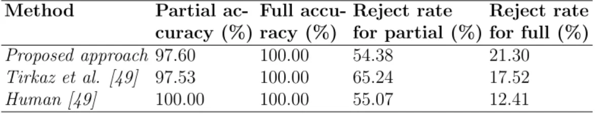
To achieve autocompletion of graphical symbols, it is necessary that the recognizer is able to recognize partially drawn symbols. Only a few methods [49, 32, 50, 51] have been introduced supporting this feature.
Only a few methods have been introduced which are able to assist the user in the completion of multi-stroke hand drawn symbols. Some of them, such as OctoPocus, [52], SimpleFlow [53] and GestureCommander [54], only work for unistroke symbol completion: by exploiting different recognition and feedback techniques, they provide the user with a visual feedback on the recognition while the gesture is still being performed. Among those working for multi-stroke symbols, a grammar-based technique is presented in [51]. In adjacency grammars, as those used in [51], primitive types are the terminal symbols and the productions describe the topology of the symbols. Furthermore, a set of adjacency constraints (e.g. incident, adjacent, intersects, parallel, perpendicular) define the relation between two primitives.
In particular, once a partial input has been processed, the parser is able to propose to the user a set of final acceptance states (valid symbols) that have as subshapes the current intermediate state. In [50] a Spatial Relation Graph (SRG) and its partial matching method are proposed for online composite graphics representation and recognition. The SRG structure is a variation of ARG in which an edge connects two nodes only if a spatial relation (interconnection, tangency, intersection, parallelism and concentricity) is present between the primitives associated to the nodes. A Spatial Division Tree (SDT) has been used in [32]. In this representation, a node in the tree contains a set of strokes. Furthermore, intersection relations among strokes are codified through links among nodes. The approach described in [49] is based on clustering. In order to assign a (possibly partial) symbol to a cluster, the set of features described in [36] is extracted from it. The features are extracted on the partially drawn symbols used in the training data. Hence, the
approach relies on the observation that people do tend to prefer certain stroke drawing orderings over others. Other, domain-specific, systems supporting symbol autocompletion have been described in literature. For instance, [55] describes a system for the recognition of a set of 485 symbols from Course of Action Diagrams [56], which also supports autocompletion.
The first three of the above cited methods show poor performance with partially drawn symbols when only a few primitives are available. As a consequence, they might not lend themselves well for the realization of an interactive system for autocompletion. The one described in [49], instead, is not completely invariant with respect to stroke order, but relies on users’ preferred order. Furthermore, the authors of the above researches do not provide evidence that symbol autocompletion can lead to a real advantage in terms of drawing time saving.
2.4
Attachment areas
Another thing related to the sketch recognition are the attachment areas. Attachment areas are the areas on which relations between symbols (of a visual language) can be defined. They are related to the physical appearance of the symbol an and can have different shapes, like a single point or parts of a symbol or an area defined by the symbol itself.
In sketch recognition research, only a few works [8] have raised the problem of correctly identifying the attachment areas. This is probably due to the lack of well established solutions to the related problems of ink segmentation and object recognition, on which most of the effort of researchers is focused. Different techniques, in fact, can be used to recognize symbols in sketched diagrams. Some of them are stroke-based, online and use time data [55], some others rely on image-based techniques [40, 36]. Other researches also try to solve the segmentation problem related to the separation of symbols from other elements of the diagrams, such as connectors. E.g., in [35] the areas of high ink density are likely to be recognized as symbols instead of connectors. The management of attachment areas is often defined ad hoc for the considered domain.
2.5
Euler diagram sketching
Methods and tools have been developed for the recognition of specialized diagrams, e.g. in engineering, chemistry, medicine, music and so on [57, 1, 58, 59]. Examples of use of sketch recognition include graphical environments for hand-drawing Euler diagrams (EDs). Previous works on ED sketch recognition [60, 61, 62] utilize single stroke recognition and machine learning techniques. In particular, in [60], the authors present a sketch tool for drawing EDs through ellipses, with a recognition mechanism able to extract the semantic of a sketched ED and to convert it into a formal diagram drawn with circles and ellipse. This work is extended in [61] by including the support to arbitrary closed curves, input and editing in the formal view, production of sketches from formal diagrams, and semantic matching via the computation of abstract representations. In [62], the authors presents a sketch tool for the recognition of EDs augmented with graphs and shading.
Chapter 3
RankFrag: a Novel Technique
for Corner Detection in Hand
Drawn Sketches
Sketched diagrams recognition raises a number of issues and challenges, in-cluding both low-level stroke processing and high-level diagram interpretation [63]. A low-level problem is the segmentation (also known as fragmentation) of input strokes. Its objective is the recognition of the graphical primitives (such as lines and arcs) composing the strokes. Stroke segmentation can be used for a variety of objectives, including symbol recognition in structural methods [34, 11].
Most approaches for segmentation use algorithms for finding corners, since these points represent the most noticeable discontinuity in the graphical strokes. Some other approaches [25] also find the so called tangent vertices (smooth points separating a straight line from a curve or parting two curves).
A high accuracy and the possibility of being performed in real time are crucial features for segmentation techniques. Tumen and Sezgin [23] also emphasize the importance of the adaptation to user preferences and drawing style and to the particular domain of application. Adaptation can be achieved by using machine learning-based techniques. Machine learning has also proven to improve accuracy. In fact, almost all of the most recent segmentation
methods use some machine learning-based technique.
The technique presented here, called RankFrag, uses machine learning to decide if a candidate point is a corner. This technique is strongly inspired to previous work. In particular, the work that mostly influenced this research is that of Ouyang and Davis [1], which introduced a cost function expressing the likelihood that a candidate point is a corner. A distinguishing feature of the presented technique is the so called rank of a candidate point. Points with a higher rank (a lower integer value) are more likely to be corners. The rank is a progressively decreased integer value, assigned to the points as they are iteratively removed from a list of candidate corners. At each iteration, the point minimizing Ouyang and Davis’s cost function is removed from the list. Another important characteristic of RankFrag is the use of a variable “region of support” for the calculation of some local features, which is the neighborhood of the point on which the features are calculated. Most of the features used for classification are taken from several previous works in the literature [64, 65, 20, 66, 1].
RankFrag has been tested on three different data sets previously introduced and already used in the literature to evaluate existing techniques. The performance of RankFrag has been compared to other state-of-art techniques [21, 23] and significantly better results are achieved on all of the data sets.
The chapter is organized as follows: Section 3.1 describes RankFrag; Section 3.2 presents the evaluation of its performance in comparison to those of existing techniques, while the results are reported in Section 3.3; lastly, some final remarks conclude the chapter.
3.1
The RankFrag technique
As a preliminary step, the stroke is processed by resampling its points to obtain an equally spaced ordered sequence of points P = (p1, p2, . . . , pn),
where n varies depending on a fixed space interval and on the length of the stroke. To extract equally spaced points the procedure described in [30] is used. Furthermore, a Gaussian smoothing [67] is executed on the extracted points in order to reduce the resampled stroke noise.
In order to identify the corners, the following three steps are then executed:
1. Initialization;
2. Pruning;
3. Point classification.
The initialization step creates a set D containing n pairs (i, c), for i = 1 . . . n where c is the cost of pi and is calculated through Equation 3.1 derived
from the cost function defined in [1].
Icost (pi) =
mse(S; pi−1, pi+1) × dist (pi; pi−1, pi+1) if i ∈ {2, . . . , n − 1}
+∞ if i = 1 or i = n
(3.1) In the above equation, S = {pi−1, pi, pi+1} and mse(S; pi−1, pi+1) is the
mean squared error between the set S and the line segment formed by (pi−1, pi+1). The term dist (pi; pi−1, pi+1) is the minimum distance between pi
and the line segment formed by (pi−1, pi+1). Since p1 and pn do not have a
preceding and successive point, respectively, they are treated as special cases and given the highest cost.
The pruning step iteratively removes n − np elements from D in order to make the technique more efficient. The value np is the number of candidate corners not pruned in this step and depends on the data sets. It is chosen so that no corner is eliminated in the pruning step. At each iteration, the element m with the lowest cost is removed and the costs of the closest preceding points ppre in P and the closest successive point psuc in P of pm, with pre and
suc occurring in D, are updated through Equation 3.2.
Cost (pi) =
mse(S; pipre, pisuc) × dist (pi; pipre, pisuc) if i ∈ {2, . . . , n − 1}
+∞ if i = 1 or i = n
(3.2) The points pipre and pisuc are, respectively, the closest preceding and successive
between pipre and pisuc in the resampled stroke P . The functions mse and
dist are defined as for Equation 3.1.
The point classification step returns the list of points recognized as corners by further removing from D all the indices of the points that are not recognized as corners. This is achieved by the following steps:
1. find the current element in D with minimum cost (if D contains only 1 and n, return an empty list);
2. calculate the features of the point corresponding to the current element and determine if it is a corner by using a binary classifier, previously trained with data.
if it is not a corner, delete it from D, make the necessary updates and go to 1.
if it is a corner, proceed to consider as current the next element in D in ascending cost order, if such a point is the first or the last point return the list of points corresponding to the remaining elements in D (except for 1 and |P |), otherwise go to 2.
In Fig. 3.1, the function DetectCorners() shows the pseudocode for the initialization, pruning and point classification steps. In the pseudocode, D is the above described set with the following functions:
Init(L) initialize D with all the (i, c) pairs contained in L; FindMinC() returns the element of D with the lowest cost;
PreviousI(i) returns j such that (j, c′) is the closest preceding element
of (i, c) in D, i.e., j = max{k | (k, c) ∈ D and k < i};
SuccessiveI(i) returns j such that (j, c′) is the closest successive
element of (i, c) in D, i.e., j = min{k | (k, c) ∈ D and k > i};
SuccessiveC(i) returns the successive element of (i, c) in D with respect to the ascending cost order;
Input: an array P of equally spaced points that approximate a stroke, a number np of not-to-be-pruned points, and the Classifier() function.
Output: a list of detected corners.
1: function DetectCorners(P , np, Classifier) 2: # initialization
3: for i = 1 to |P | do
4: c ← Icost(i, P ) # computes Equation 3.1
5: add (i, c) to TempList 6: end for 7: D.Init(TempList) 8: # pruning 9: while |D| > np do 10: (imin, c) ← D.FindMinC() 11: RemoveAndUpdate(imin, P , D) 12: end while 13: # point classification 14: while |D| > 2 do 15: (icur, c) ← D.FindMinC() 16: loop
17: isCorner ← Classifier(icur, P , D)
18: if isCorner then
19: (icur, c) ← D.SuccessiveC(icur)
20: if icur ∈ {1, |P |} then
21: for each i /∈ {1, |P |} in D add P [i] to CornerList
22: return CornerList 23: end if 24: else 25: RemoveAndUpdate(icur, P , D) 26: break loop 27: end if 28: end loop 29: end while 30: return ∅ 31: end function 32: procedure RemoveAndUpdate(i, P , D) 33: ipre ← D.PreviousI(i) 34: isuc ← D.SuccessiveI(i) 35: D.Remove(i)
36: c ← Cost(ipre, P , D) # computes Equation 3.2
37: D.UpdateCost(ipre, c)
38: c ← Cost(isuc, P , D)
39: D.UpdateCost(isuc, c)
40: end procedure
Figure 3.1: The implementation of the initialization, pruning and corner classification steps.
UpdateCost(i, c) updates the cost of i in D setting it to c.
DetectCorners() calls a Classifier(i, P , D) function that computes the features (described in Section 3.1.2) of the point P [i], and then uses them to determine if P [i] is a corner by using a binary classifier previously trained with data (described in Section 3.1.3).
3.1.1
Complexity
The complexity of the function DetectCorners() in the previous section depends on the implementation of the data structure D. The following calculation will be based on the implementation of D as an array in which the ith element refers to the node that contains the pair (i, c) (or nil if the node does not exist) and a pointer that refers to the node with the minimum c. Each node has 3 pointers: one that points to the successive node in ascending c order, one that points to the successive node in ascending i order and one that points to the previous node in ascending i order. With this implementation, the FindMinC(), PreviousI(), SuccessiveI(), SuccessiveC() and Remove() functions are all executed in constant time, while UpdateCost() function is O(|D|) (where |D| is the number of nodes referred in D) and the Init(L) function is O(|L| log |L|) (by using and efficient sorting algorithm). In the following, it will be shown that the DetectCorners() complexity is O(n2),
where n = |P |.
It is trivial to see that: the complexity of the ICost() function is O(1); the complexity of Cost() is O(n) in the worst case and, consequently, the complexity of RemoveAndUpdate() is O(n); and the complexity of Clas-sifier() is O(n) since some features need O(n) time in the worst case to be calculated.
The complexity of each of the three steps is then:
1. Initialization: ICost() is called n times and D.Init() one time, conse-quently the complexity of the initialization step is O(n log n).
2. Pruning: D.FindMinC() and RemoveAndUpdate() are called n−np times each, consequently the complexity of this step is O(n(n − np)).
3. Point classification: the while loop (in line 14) will be executed at most k = |D| − 2 ≤ np − 2 times. In the loop (in line 16), Classifier() will be called at most k times, D.SuccessiveC() at most k − 1 times, and RemoveAndUpdate() at most once. Thus, in this step, they will be called less or equal than k2, k2 and k times, respectively.
The complexity of the Classifier() calls can be calculated by consid-ering that for each point, if none of its features changes, the result of Classifier() can be retrieved in O(1) by caching its previous output. Since the execution of the RemoveAndUpdate() function involves the changing of the features of two points, Classifier() will be executed at most 3k times in O(n) (for a total of O(k × n)) and the remaining times in O(1) (for a total of O(k2)), giving a complexity of O(k × n). Furthermore, the complexity of the D.SuccessiveC() calls is O(k2),
while the complexity of the RemoveAndUpdate() calls is O(k × n). Thus, since k < n, the point classification step is in the worst case O(k × n), or rather O(n × np).
It is worth noting that the final O(n2) complexity does not improve even if a
better implementation of D providing an O(log |D|) UpdateCost() function is used.
3.1.2
Features
The main distinguishing feature used by the presented technique is the rank. The rank of a point p = P [i], with respect to D, is defined as the size of D resulting from the removal of (i, c) from D. The other features are derived from previous research in the field. There are three different classes of features:
Stroke features: features calculated on the whole stroke;
Point features: local features calculated on the point. These features are calculated using a fixed region of support and their value remain stable throughout the procedure;
Rank-related features: dynamically calculated local features. The region of support for the calculation of these features is the set of points from the predecessor ppre and the successor psuc of the current point in the
candidate list. Their value can vary during the execution of the Point classification step.
Stroke Features
The features calculated on the whole stroke can be useful to the classifier, since a characteristic of the stroke can interact in some way with a local feature. For instance, the length of a stroke may be correlated to the number of corners in it: it is likely that a long stroke has more angles than a short stroke. Two stroke features are derived from [1]: the length of the stroke and the diagonal length of its bounding box. These features are called Length and Diagonal , respectively. Furthermore, a feature telling how much the stroke resembles an ellipse (or a circle), called EllipseFit , was added. It is calculated by measuring the average euclidean distance of the points of the stroke to an ideal ellipse, normalized by the length of the stroke.
Point Features
The point features are local characteristics of the points. The speed of the pointer and the curvature of the stroke at a point have been regarded as very important features from the earliest research in corner finding. Here, the speed at pi is calculated as suggested in [64], i.e., s(pi) = ∥pi+1, pi−1∥ /ti+1− ti−1,
where ti represents the timestamp of the i-th point. It is also present a version
of the speed feature where a min-max normalization is applied in order to have as a result a real value between 0 and 1; the Curvature feature used here is calculated as suggested in [65].
A feature that has proven useful in previous research is the straw, proposed in [20]. The straw at the point pi is the length of the segment connecting
the endpoints of a window of points centered on pi. Thus Straw (pi, w) =
∥pi+w, pi−w∥, where w is the parameter defining the width of the window.
the angle formed by the segments (pi−w, pi) and (pi, pi+w(, defined here as
Angle(pi, w). A useful feature to distinguish the curves from the corners is
called AlphaBeta, derived from [21]. alpha and beta are the magnitudes of two angles in pi using different segment lengths, one three times the other.
Here the difference between them is used as a feature: AlphaBeta(pi, w) =
Angle(pi, 3w) − Angle(pi, w).
Lastly, in this research two point features are introduced, that, to the best of my knowledge, have never been tested so far for corner detection. One feature is the position of the point within the stroke, indicated as the ratio between the length of the stroke from p0 to pi and the total length
of the stroke. This feature is called Position(pi). The other feature is the
difference of two areas: the former is the one of the polygon delimited by the points (pi−w, . . . , pi, . . . , pi+w( and the latter is the one of the triangle
(pi−w, pi, pi+w). The rationale for this feature is that its value will be positive
for a curve, approximately 0 for an angle and even negative for a cusp. It is called DeltaAreas(pi, w).
Rank-Related Features
The rank-related features are local characteristics of the points. The difference with the point features is that their region of support varies according to the rank of the point: the considered neighborhood is between the closest preceding and successive points of pi occurring in D, which are called pipre
and pisuc, respectively. The Rank and the Cost function defined in Equation
(3.2) are examples of features from this class.
A simple feature derived from [1] is MinDistance, representing the mini-mum of the two distances ∥pipre, pi∥ and ∥pi, pisuc∥, respectively. A normalized
version of MinDistance is obtained by dividing the minimum by ∥pipre, pisuc∥.
As in previous research, parts of the stroke are tried to be fitted with beau-tified geometric primitives. The following two features are inspired by the ones defined in [66]: PolyFit (pi) tries to fit the substroke (pipre, . . . , pi, . . . , pisuc)
with the polyline (pipre, pi, pisucc), while CurveFit (pi) uses a bezier curve to
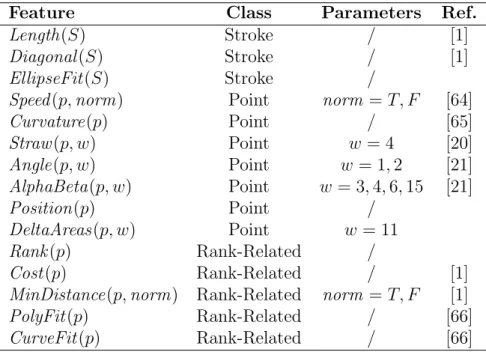
Feature Class Parameters Ref.
Length(S) Stroke / [1]
Diagonal (S) Stroke / [1]
EllipseFit (S) Stroke /
Speed (p, norm) Point norm = T, F [64]
Curvature(p) Point / [65] Straw (p, w) Point w = 4 [20] Angle(p, w) Point w = 1, 2 [21] AlphaBeta(p, w) Point w = 3, 4, 6, 15 [21] Position(p) Point / DeltaAreas(p, w) Point w = 11 Rank (p) Rank-Related / Cost (p) Rank-Related / [1]
MinDistance(p, norm) Rank-Related norm = T, F [1]
PolyFit (p) Rank-Related / [66]
CurveFit (p) Rank-Related / [66]
Table 3.1: The features used in RankFrag.
distance normalized by the length of the stroke.
Table 3.1 summarizes the set of features used by RankFrag in the Classi-fier function. The table reports the name of the feature, its class, the values of the parameters (if present) with which it is instantiated and the reference paper from which it is derived. The presence of feature parameters means that some feature could potentially be used several times, instantiated with a different parameter value, and this might introduce redundant features. The parameters have been chosen by performing an internal validation process that measures the relevance of the parameter-dependent features, over possible parameter values, and uses feature clustering to define a subset of relevant, non-redundant features.
3.1.3
Classification method
The binary classifier used by RankFrag in the Classifier function to classify corner points is based on Random Forests (RF) [68]. Random Forests are an ensemble machine learning technique that builds forests of classification trees. Each tree is grown on a bootstrap sample of the data, and the feature
at each tree node is selected from a random subset of all features. The final classification is determined by using a voting system that aggregates the classification results from all the trees in the forest. There are many advantages of RF that make their use an ideal approach for this classification problem: they run efficiently on large data sets; they can handle many different input features without feature deletion; they are quite robust to overfitting and have a good predictive performance even when most predictive features are noisy.
3.1.4
Implementation
RankFrag was implemented as a Java application. The classifier was imple-mented in R language, using the randomForest package [69]. The call to the classifier from the main program is performed through the Java/R Interface (JRI), which enables the execution of R commands inside Java applications.
3.2
Evaluation
RankFrag was evaluated on three different data sets already used in the literature to evaluate previous techniques. A 5-fold cross validation was repeated 30 times on all of the data sets. For all data sets, the strokes were resampled at a distance of three pixels, while a value of np = 30 was used as a parameter for pruning. Since there is no single metric that determines the quality of a corner finder, the performance of RankFrag was calculated using the various metrics already described in the literature. The results for some metrics were averaged in the cross validation and were summed for others.
The hosting system used for the evaluation was a laptop equipped with an IntelCorei7-2630QM CPU at 2.0 GHz running Ubuntu 12.10 operating system and the OpenJDK 7.
3.2.1
Model validation
This section describes the process of assessing the prediction ability of the RF-based classifiers. The accuracy metrics were calculated by repeating 30
times the following procedure individually for each data set and taking the averages:
1. the data set DS is divided randomly into 5 parts with an equal num-ber of strokes (or nearly so, if the numnum-ber of strokes is not divisible by 5);
2. for i = 1 . . . 5: DSti = ∪(DSj) {j ̸= i} is used as a training set, and
DSi is used as a test set.
RankFrag is executed on DSti in order to produce the training
data table. In DS , the correct corners had been previously marked manually. For each point extracted from the candidate list the input feature vector is calculated, while the output parameter is given by the boolean value indicating whether the point is marked or not as a corner. The training table contains both the input and output parameters;
A random forest is trained using the table;
RankFrag is executed on DSi, using the trained random forest as
a binary classifier;
In order to generate the accuracy metrics, the corners found by the last run of RankFrag are compared with the manually marked ones. A corner found by RankFrag is considered to be correct if it is within a certain distance from a marked corner (only one corner found by RankFrag can be considered to be correct for each marked corner).
3. In order to get aggregate accuracy metrics, for each of them the aver-age/sum (depending on the type of the metric) of the values obtained in the previous step is calculated.
3.2.2
Accuracy metrics
A corner finding technique is mainly evaluated from the points of view of accuracy and efficiency. There are different metrics to evaluate the accuracy of a corner finding technique. The following metrics, already described in the literature [20, 22], are used:
False positives and false negatives. The number of points incor-rectly classified as corners and the number of corner points not found, respectively;
Precision. The number of correct corners found divided by the sum of the number of correct corners and false positives:
precision = correct corners+false positivescorrect corners ;
Recall. The number of correct corners found divided by the sum of the number of correct corners and false negatives:
recall = correct corners
correct corners+false negatives.
This value is also called Correct corners accuracy;
All-or-nothing accuracy. The number of correctly segmented strokes divided by the total number of strokes;
The task of judging whether a corner is correctly found is done by a human operator. The presence of the angle is then determined by human perception. Obviously, different operators can perform different annotations on a data set. In this work, data sets already annotated by other authors are used. It is worth noting that a tolerance of 7 sampled points (corresponding to a maximum distance of 21 pixels) from the marked corner was used. This value is similar to others used in the literature (e.g., in [22] a fixed distance of 20 pixels was used).
3.2.3
Data sets
Two of the three data sets used in this evaluation, the Sezgin-Tumen COAD Database and NicIcon data sets, are associated to a specific domain, while
Data set No. of No. of No. of No. of Source
classes symbols strokes drawers
COAD* 20 400 1507 8 [49]
NicIcon 14 400 1204 32 [70]
IStraw 10 400 400 10 [21]
Table 3.2: Features of the three data sets.
the IStraw data set is not associated to any domain, but it was produced for benchmarking purposes by Xiong and LaViola [21]. Some features of the three data sets are summarized in Table 3.2. The table reports, for each of them, the number of different classes, the total number of symbols and strokes, the number of drawers and a reference to the source document introducing it. The Sezgin-Tumen COAD Database (called only COAD*, for brevity, in the sequel) is composed by 400 symbols (1507 strokes with their identified corners) extracted from the COAD data set described in Appendix A.4. The NicIcon and IStraw data sets are described in the Appendix A.2 and Appendix A.1, respectively.
3.3
Results
This section reports the results of the RankFrag evaluation. As for the accuracy, all of the metrics described in the previous section were calculated. Furthermore, RankFrag’s accuracy is compared to that of other state-of-art methods by using the All-or-nothing metric. It is worth noting that, due to the unavailability of working prototypes, the other methods are not directly tested: only the performance declared by their respective authors are reported.
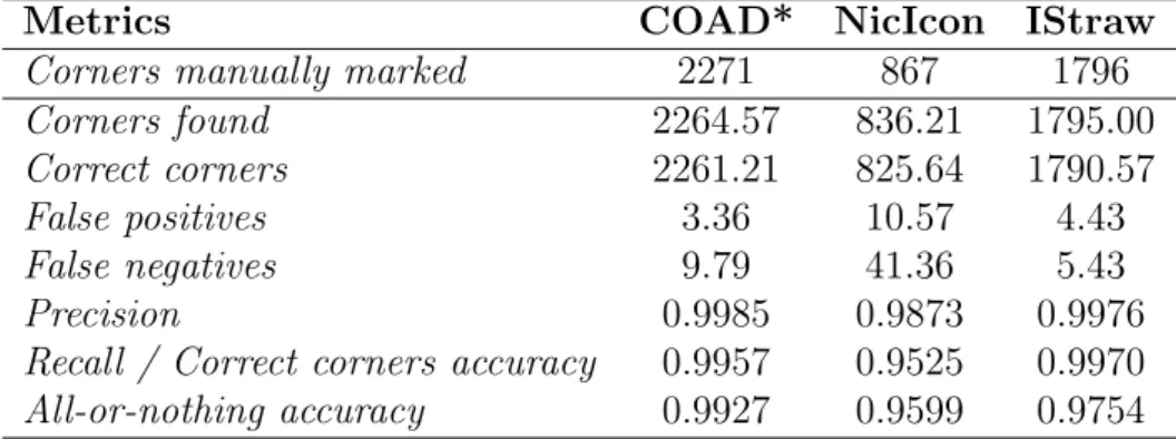
The accuracy achieved by RankFrag on the three data sets is reported in Table 3.3. The results are averaged over the 30 performed trials.
Table 3.4 shows a comparison of the accuracy of RankFrag with other state-of-art methods. The methods considered here are DPFrag [23] and IStraw [21]. Due to the unavailability of other data, only the results related to the All-or-nothing metric are reported.
Metrics COAD* NicIcon IStraw
Corners manually marked 2271 867 1796
Corners found 2264.57 836.21 1795.00
Correct corners 2261.21 825.64 1790.57
False positives 3.36 10.57 4.43
False negatives 9.79 41.36 5.43
Precision 0.9985 0.9873 0.9976
Recall / Correct corners accuracy 0.9957 0.9525 0.9970
All-or-nothing accuracy 0.9927 0.9599 0.9754
Table 3.3: Average accuracy results of RankFrag on the three data sets.
Data set RankFrag DPFrag IStraw
COAD* 0.99 0.97 0.82
NicIcon 0.96 0.84 0.24
IStraw 0.98 0.96 0.96
Table 3.4: Comparison of RankFrag with other methods on the All-or-nothing accuracy metric.
largest improvement is obtained on the NicIcon data set, where the other two methods perform rather poorly. Less noticeable improvements are obtained on the COAD and on the IStraw data sets, where the other two methods do not perform badly.
As for efficiency, the average time needed to detect the corners in a stroke is ∼390 ms. This implementation is rather slow, due to the inefficiency of
the calls to R functions. A non-JRI implementation was also produced by manually exporting the created random forest from R to Java (avoiding the JRI calls). With this implementation, the average execution time is lowered to ∼130 ms, thus enabling real-time user interactions.
3.4
Concluding remarks
This chapter has introduced RankFrag, a technique for detecting corner points in hand drawn sketches. The technique outperforms two state-of-art methods on all the tested data sets. In particular, RankFrag is the only technique obtaining a satisfactory result on the “difficult” NicIcon data set, correctly
processing the 96% of the strokes.
RankFrag finds only corner points and not tangent vertices, as done by other techniques [24, 25]. It can be directly used in various structural methods for symbol recognition, as shown in Chapter 5. However in some methods an additional step to classify the segments in lines or arcs may be required.
Chapter 4
Improving Shape Context
Matching for the Recognition
of Sketched Symbols
In this chapter, an approach to recognize multi-stroke hand drawn symbols is presented. Since the approach is an adaptation of the image-based matching algorithm proposed by Belongie et al. [2], it is invariant with respect to scaling and is independent from the number and order of the drawn strokes. Furthermore, it has a better recognition accuracy than the original one when applied to hand drawn symbols. This is due to the exploitation of information on stroke points, such as temporal sequence and occurrence in a given stroke.
Briefly, the algorithm proposed by Belongie et al. calculates the matching cost between two shapes as the minimum weighted bipartite graph matching between two equally sized sets of sampled points from both shapes. This is done by calculating a matrix of matching costs between each couple of points of the two symbols and selecting the resulting best match. The cost of matching of two points is calculated by evaluating the difference between their shape contexts, which are suitable shape descriptors introduced by the authors.
The approach improvement lies in re-calculating the cost matrix and, as a consequence, the total cost of matching between the two symbols. The cost