RICERCA DI SISTEMA ELETTRICO
Development of a multi-scale methodology for composite structural
modelling and validation of modelling procedure by mechanical testing -
Final Report
Andrea MorianiReport RdS/2012/268
Agenzia nazionale per le nuove tecnologie, l’energia e lo sviluppo economico sostenibile
DEVELOPMENT OF A MULTI-SCALE METHODOLOGY FOR COMPOSITE STRUCRTURAL MODELLING AND VALIDATION OF MODELLING PROCEDURE BY MECHANICAL TESTING – FINAL REPORT
Andrea Moriani (ENEA)
Settembre 2012
Report Ricerca di Sistema Elettrico
Accordo di Programma Ministero dello Sviluppo Economico - ENEA Area: Governo, gestione e sviluppo del sistema elettrico nazionale
Progetto: 1.3.2 Fusione nucleare: attività di fisica e tecnologia della fusione complementari a ITER Responsabile del Progetto: Aldo Pizzuto, ENEA
3 Indice
Sommario ... 4
1. Introduction ... 5
2. Method to represent the results about a progressive failure model in composite materials ... 5
3. Selection of the environment for the development ... 14
4. Constitutive model for a balanced plain weave fabric ... 22
5. Validation of the model by testing ... 47
6. Conclusions ... 63
Appendix 1 ... 65
Classical laminate theory applied to tensile load tests ... 65
Sommario
Objectives of the work are to develop a multiscale methodology for composite structural modelling and to validate the modelling procedure by mechanical testing.
In the field of the computational material science the multiscale methodology plays an important role. It is based on the hierarchical concept which recognises that there is a strong interconnection between phenomena which happen to different scales of length and time. In the field of the composite material the approach consists in the description of the ply by knowing the behaviour of the constituents, i.e. fibre and matrix.
In this work was developed a constitutive model for a balanced plain weave fabric. This model, starting from geometrical parameters and mechanical parameters of the single constituents (fibre and matrix), determines the effective moduli of the representative unit cell (RUC). This model was implemented into a general purpose finite element program ABAQUS, building a specific user subroutine.
The last part of this job was to determine a material failure mechanism theory for the balanced plain weave architecture that was implemented in the same specific user subroutine. The prediction of the failure at each increment of the load was obtained by using a quadratic failure criterion, applied to the strains with stiffness and strength reduction scheme to account for damage within the yarns.
This standard user subroutine is an augmentation for any commercial finite element code giving the possibility to deal with any composite material made with balanced plain weave fabric, knowing the mechanical properties of the single constituents and the specific failure mechanism.
5 1. Introduction
A technique to describe the mechanical behaviour of the composite materials is the multiscale methodology, which allows to link the macroscopic behaviour with the micro-structural characteristics and it results to be a more predictive approach (with respect to phenomenological models) with the possibility to estimate the effect of a change in the fibres and matrix arrangement on the composite behaviour. Practically, the approach consists in the description of the behaviour at the scale of the constituents, fibre and matrix, (microscale) where each constituent is modelled by using continuum mechanics relationships. Afterwards, the homogenisation treatment will allow to create a mesoscale structure (e.g., layer) and finally to deduce the macroscopic behaviour. The findings and results of this study can be implemented in a finite element code by means of a user subroutine. A similar approach can be attempted for thermal properties.
An important part of the task is the validation of the modelling by testing. These tests are aimed both at the determination of the basic constituent properties (fibre and matrix), fibre-matrix interface behaviour and at composite macroscopic properties. The tests include fibre tensile and composite tensile, compression, shear and bending.
2. Method to represent the results about a progressive failure model in composite materials
We have started to study the argument of the design of composite materials using a general purpose finite element program named ABAQUS. Laminated composite structures under load develop local failures such as matrix cracks, fiber breakage and fibre matrix debonds, which are termed as damage. These effects cause permanent loss of stiffness and strength of the material. It becomes important to predict the initiation and growth of such damage for assessing the performance of composite structures.
The analysis of composite laminates is complicated because of both material and geometric non-linearity, that came into play when the loads are increased beyond the first ply failure. Material non-linearity results from the damage mentioned early, and the geometric non-linearity is due to large displacements experienced by the structure during loading.
Commercial code gives to the user tools to deal with composite materials. For two-dimensional models there is shell element based on first order shear deformation theory, that have better performance in large deformation analysis. The strain state is referred to a specific coordinate system and the stacking sequence of the laminate is specified to this reference coordinate system.
As we have just said damage in composite materials plays an important role. To study these behaviours is used a progressive failure method, where the load is
applied incrementally during the analysis. At each load step, a geometric non-linear analysis is performed until a converged solution is obtained. Knowing the deformation and stress states at each material integration point, it become possible to compare these result with material allowable stress. If failure is detected, stiffness reduction is carried out at the integration Gauss points of the finite element mesh depending on the mode of failure. However, it is not an easy task to determine the degraded properties of the damaged material with certainty.
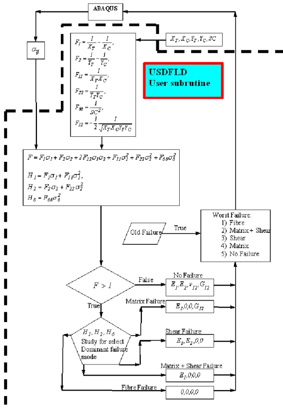
The user can define material properties as functions of the field variables at a material point using specific user subroutine.
The need to write specific software that represents an augmentation for any commercial finite element code, gives a big problem to the user in the representation of the results of the analysis. Where is the first ply failure and how the progression of the damage develops, these are some questions that the users have to answer.
In this paragraph is implemented a progressive failure method into the general purpose finite element program, ABAQUS. A specific application is developed for a post processing visualization of the results.
We have studied a panel, made of five unidirectional plies, where all the edges are clamped and the load is a uniform pressure applied to the bottom surface (Figure 2.1).
Figure 2.1: Plate geometry.
The plate specification is shown in Table 2.1 and the material properties are shown in Table 2.2. The orthotropic material properties of a lamina are obtained either by the theoretical approach or through suitable laboratory tests. The
7
theoretical approach, called a micromechanics approach, that relate the fiber and matrix contributions to the properties of complete structures.
A typical procedure for a progressive failure analysis is illustrated in figure 2.2. The preprocessing phase is built in the standard ABAQUS environmental and a specific user subroutine USDFLD was written, which allows the user to define material properties as functions of the field variables at a material point.
Table2.2: Mechanical properties of unidirectional E-Glass/Polyester ply Longitudinal Modulus, Ex
GPa
23.6 Transverse Modulus, Ey Ez
GPa
10.0Shear Modulus, Gxy
GPa
1.0Poisson’s ratio, xy 0.23
Longitudinal Tensile Strength, XT
MPa
735.0Longitudinal Compressive Strength, XC
MPa
600.0 Transverse Tensile Strength, YT
MPa
45.0Transverse Compressive Strength, YC
MPa
100.0 In-Plane Shear Strength, SC
MPa
45.0Table 2.1: Laminate plate specifications
Lay-up Sequence Number of Plies Length
mm Width
mm Thickness
mmFigure 2.2: Progressive failure analysis.
The full plate is modelled using 20x20 four node shell element S4R of the ABAQUS element library based on first order shear deformation theory. How is shown in figure 2.3 with the subroutine USDFLD it is possible to incorporate in ABAQUS the TSAI-WU criterion:
1 F 6 1 6 1 6 1
i j j i ij i i i F F (2.1)Finite Element Program ABAQUS Moduli Parameters: xy xy z y x,E ,E ,G , E User subroutine USDFLD Strength Parameters SC , Y , Y , X , XT C C C Results
9
Figure 2.3: Progressive failure analysis.
Load P(i)
Geometrically Nonlinear Analysis to Establish Equilibrium
Converged Solution Obtained Define Initial
State
Compute Stresses/Strains at All the Gauss Points
Check for Failure at all the Gauss Points Failure Detected ? Increment Load P(i)=P(i)+P Predicted Failure Load Stop Re- Establish Equilibrium Degrade Material Properties at Failed Gauss Points Small P
USDFLD
1 F F F 6 1 i 6 1 j ij i j 6 1 i i i Yes No No Yes TSAI-WU Criterion:Where i denotes the stress components referred to the principal material
coordinates and the parameters F are function of the lamina normal tension and
shear strengths. At each load step, Gauss point stresses are used in the failure criterion. If failure occurred at a Gauss point, a modification of the lamina properties was made at that Gauss point, which results in reduced stiffness of the laminate. To this purpose the following expressions are used to determine the failure mode:
2 1 11 1 1 1 F F H 2 2 22 2 2 2 F F H (2.2) 2 6 66 6 F H
The largest term is selected as the dominant failure mode and the
corresponding modulus is reduced to zero. In particular H1 corresponds to fibre
failure, H2 corresponds to matrix crack and H6 corresponds to fibre matrix shearing
failure. The code implemented in the user subroutine is shown in the flow chart reported in figure 2.4.
11
Figure 2.4: Progressive failure analysis.
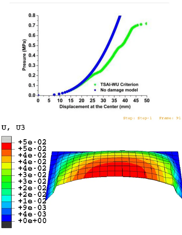
In figure 2.5 are reported results of the analysis using the standard post processing tools in ABAQUS.
Figure 2.5: Standard ABAQUS representation.
To the top there is the load central deflection graph and to the botton there is a picture of the deformation of a half part of the plate. But with the standard tools is impossible to visualize where the first ply failure is and how the progression of the damage develops. To answer to these questions we have developed a specific application for post processing visualization of the results.
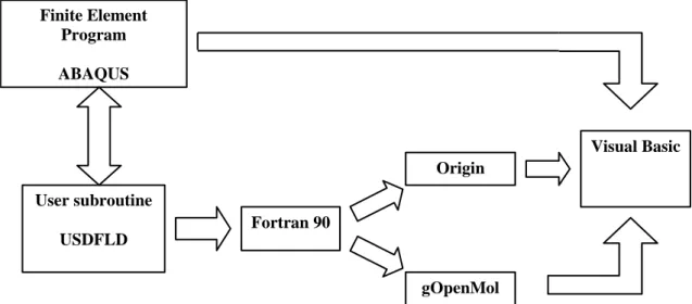
13
Used data came from the user subroutine USDFLD and such data have been elaborated through programs written in Fortran 90 whose files of exit have been visualized through the programs of graphic analysis Origin and gOpenMol. Then a specific program was written in Visual Basic that has allowed visualizing all the results of the post elaboration.
The scheme is reported in figure 2.6.
Figure 2.6: Flow chart of the post processing phase. The graphical user interface used in Visual Basic is shown in figure 2.7.
A pressure increase of 0.008 MPa is used for the analyses and the number of load step is 89.
To the right top there is the load central deflection graph and on its left it is possible to see the move of the deformation of a half part of the plate. To the bottom there are representations of the failure mode with the indication of the percent of the material point with that failure and the number for every play. There is also a graphical representation of the defect positions. Pushing the start button the representation of the time progression of the simulation begins. It is also possible to change the time between two steps. In the graphs horizontal lines show the load that is reached during the progression of the simulation.
Finite Element Program ABAQUS User subroutine USDFLD Fortran 90 Origin gOpenMol Visual Basic
Figure 2.7: Graphical user interface in Visual Basic.
The first ply failure was due to matrix cracking and started from the bottom surface. The drastic change in the central deflection around the pressure of 0.20 MPa is due to the rapid increase of the matrix cracking failure while the change at 0.46 MPa is imputable at the start of the fiber breakage failure. Then the pressure increases bring to a structural collapse due to the fiber breakages spread through the thickness.
In this first approach to the composite material analysis we have developed into one general purpose finite element program a progressive failure methodology for composite plates and we have implemented a specific application to show the type and extent of the damage at a given load, the first ply failure load and the final collapse load.
3. Selection of the environment for the development
The strong limitation in the standard finite element codes, in studying composite materials using multiscala methodology, have led us to seek commercial codes that we could add the necessary micro-scale analysis in a standard finite element software.
15
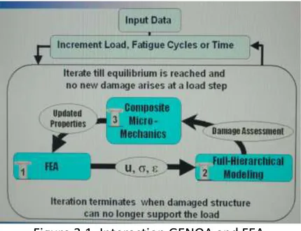
The progressive failure method is used on the design of composite materials. In a typical finite element analysis (FEA), failure is assessed at the macro-scale. On the other hand, it is well known that the initiation of damage in composite materials occurs at micro-scale. In commercial there are finite element codes based on computational composite engineering micromechanics that could be a good solution for ours task, therefore develop a multi-scale methodology for composite structural modelling. One of this is GENOA-PFDA (Progressive Failure Dynamic Analysis). Displacement, stress and strain field in a structure are obtained from the finite element solution. The corresponding response fields at the laminate and lamination (macro) scales are calculated using enhanced classical laminated theory. Most of the commercial finite element programs operate strictly at this level. Because the initiation of damage in composite materials occurs at micro-scale (fiber/matrix level), GENOA-PFDA utilized the hierarchical approach illustrated in figure 3.1. The hierarchical modelling reaches down to micro-scale level through the subdivision of unit cells (that in these reports will call RUC representative unit cell) composed of the fiber bundles and surrounding matrix material.
Stress-strain field at the micro-scale are calculated on the basis of macro-scale results, using the computational composite engineering micromechanics. The volume elements of the unit cell are interrogated for possible damage using a set of failure criteria. Once damage at the unit cell level has been detected, GENOA-PFDA degrades the relevant fiber/matrix mechanical properties based on the rules of material behaviour and experience. The accumulation of damage at the micro-level eventually leads to the fracture at the lamina (macro) level. Because damage is tracked at the micro-scale, it is possible to have several types of damage in a particular ply.
The composites and ceramics fail is due to damage growth and accumulation in the fibres, matrix or fiber/matrix interface. Damage growth is driven by increasing load, fatigue cycles, creep or environmental effects. Other affecting damage growth rates are manufacturing flaws, voids and residual stresses, moisture and temperature. Predicting composite structure failure, durability and life it means predicting composite behaviour at the micro-scale of fiber and matrix, translaminar and interlaminar.
GENOA is an augmentation to FEA adding the necessary micro-scale analysis that gives the possibility of asses the composite failures where they initiate therefore in the fiber, matrix and fiber-matrix interface.
The main components in GENOA are: 1) Progressive Failure Analysis (PFA) 2) Material Constituent Analyzer (MCA) 3) Material Uncertainty Analyzer (MUA)
4) Time Dependent Reliability (TDR)
This code is based on three main functional components:
1) Finite Element Software FEA where is used any commercial software package NASTRAN, ABAQUS, ANSYS, etc.
2) Full Hierarchical Modelling which goes down to the sub-scale. 3) Micro-Mechanics Materials Engineering.
In figure 3.1 it is shown the interaction of GENOA and FEA to perform progressive damage analysis.
Figure 3.1: Interaction GENOA and FEA.
The FEA solution give displacements (u), stresses () and strains (), with these
data the Full-Hierarchical Modelling can determine the damage to the level of the fibre and matrix and this information is passed to the Composite Micro-Mechanics which update the stiffness and strength of the fibre and matrix which are the new input for the FEA.
In the figure 3.2 there is a different view of the same process. Above the dot line there is the traditional FEA and lamina theory. Below the line are the capability added by GENOA, there is a unit cell made up of matrix and fiber furthermore, such unit cell is further divided into slice on which is applied the micro-scale analysis.
17
Figure 3.2: Capability added by GENOA to a traditional FEA.
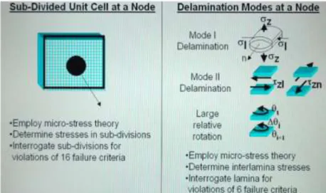
This sub-division is shown in figure 3.3 where at the slide level is employ micro-stress theory that determines where the failures are taking place in the fibre or in the matrix using 16 failure criteria. There are also 6 criteria for assessing the occurrence of delamination between the lamina.
Figure 3.3: Sub-division of the unit cell and mode of delamination. All the failure criteria are shown in figure 3.4.
Figure 3.4: Failure criteria.
Close form equations, built at micro-scale level, allow to obtain damage and the consequent reduction of stiffness and strength quickly and then the FEM can run again to assess what happening in the next step of increase of the load.
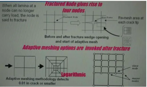
When there is a failure in a particular node (figure 3.5) of the lamina, the code must take into account that the node can no longer bear a load.
Figure 3.5: Route information of damage from the microscale to the macroscale. That node is called fractured so the code removes the node. We need to remesh and GENOA automatic remesh (figure 3.6).
19
Figure 3.6: Outline of the automatic remesh. In figure 3.7 is shown the input and the output of GENOA.
Figure 3.7: Outline of the input and the output in the GENOA code.
The code must be calibrated by knowing the properties of the fibers and matrix. When there is uncertainty on these data it becomes necessary to perform some mechanical tests on specimen of lamina or laminate as shown in figure 3.8.
Figure 3.8: Test necessary to calibrate the code.
As it can be seen in figure 3.9 the test results are input to a routine that exists in GENOA, that provides as an output the properties of the fiber and matrix.
Figure 3.9: Outline for determining the mechanical properties of the fiber and the matrix.
The module named Material Constituent Analyzer (MCA) shown in figure 3.9 calculates lamina (ply) and laminate composite properties knowing the composite architectures and a first estimation of the properties of the fiber and matrix.
21
Figure 3.10: Automated sensitivity analysis.
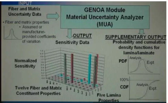
The Sensitivity Analysis, shown in figure 3.9 and in more detail in figure 3.10, is based on the module Material Uncertainty Analyzer (MUA).
This module combines micro-mechanics and probabilistic analysis for study the influence of fundamental primitive variables on the structural response and in particular, on the response sensitivity to constituent material and to other design variables, such as fiber architecture, manufacturing tolerances and defect content. The output of this module are utilized from the Time Dependent Reliability (TDR) for predict the composite system probability of failure and the sensitivity effects of the material properties, loading conditions and service and manufacturing conditions, so it will be possible targeting design parameter changes, that will be most effective in reducing probability of a given failure mode from occurring, and the probability of failure.
GENOA handles a broad spectrum of composite textile architectures (figure 3.11).
4. Constitutive model for a balanced plain weave fabric
The research for a possible commercial environmental had shown that in commercially there are finite element codes based on computational composite engineering micromechanics that could be a good solution for our problems. After the research what emerges is that such products are almost totally developed from the NASA ((National Aeronautics and Space Administration) and when commercialized they are characterized by exorbitant costs.
The high cost of the commercial code that could represent a possible environment for development of a model for the structural analysis of ceramic matrix composite material, has brought us to the decision to internally develop a multiscale code based on the commercial software ABAQUS.
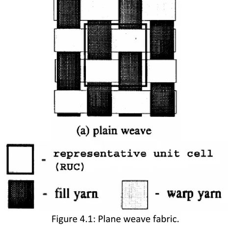
This work deals of developing a constitutive model for balanced plain weave fabric (figure 4.1). The micromechanical model was implemented in Fortran [1] programs and user material subroutine for ABAQUS [2], called UMAT, was created out of these programs.
Figure 4.1: Plane weave fabric.
This model starting from geometrical parameter and mechanical parameter of the single constituents (fiber and matrix), determines the effective moduli of the representative unit cell (RUC) shown in figure 4.2 [3].
23
Figure 4.2: Plain weave RUC geometry and notation.
This model was implemented in the structural analysis software system ABAQUS, writing a specific subroutine called UMAT. This UMAT subroutine provides the capability to combine a new material model with the powerful numerical algorithms for structural analysis available in ABAQUS.
The last part of this job was to determine a material failure mechanism theory for balanced plain weave architecture and implement this model in a specific subroutine in the ABAQUS structural analysis software.
The geometric model was developed with the following assumptions:
1. The yarn spacing (quantity a in figure 4.3) for the fill and warp yarns are
assumed to be equal.
2. There is no gap between adjacent yarns.
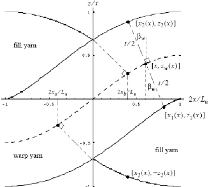
3. The centreline of the yarn path consists of undulation portions and straight portions, with the centreline of undulating portions described by the sine function as drawn in figure 4.4.
4. The cross-section area and the thickness of the yarn normal to its centreline are uniform along the arc-length of the centreline.
Figure 4.3: Cross section of the RUC along the warp yarn.
Figure 4.4: Geometry of an undulation region along the warp yarn.
The input parameters for the Fortran subroutine that solve the nonlinear equations describing the geometry of the balanced plane weave architecture are shown in the flow chart in figure 4.5.
25
Figure 4.5: Flow chart to resolve the geometry.
The first three parameters describe that the warp and fill yarns contain the same
number of filaments n, with all filaments having the same diameter df , and the
same packing density pd, that represents the ratio between the whole area of the
filaments and the yarn cross section area (figure 4.6).
FORTRAN code
All geometry parameters for the plain weave RUC (representative unit cell)
1. n = number of filaments in a yarn 2. df = diameter of a filament 3. pd = yarn packing density 4. a = yarn spacing
5. VfRUC = fiber volume fraction of the RUC (representative unit cell)
Figure 4.6: The yarn is made with n filaments.
Numerical results of the geometric model, for several values of number of filaments in a yarn, are shown in figure 4.7. In these examples the fibre volume fraction is
64 . 0
VfRUC , the diameter of a filament is df 0.007mm, the yarn spacing is
mm 411 . 1
a and the packing density is pd 0.75 while the number of filaments is
changed from 4000 to 14000. In the figure 4.7 it is possible to see the change in the geometry of the balanced plane weave as a function of the number of the filaments; and it is interesting to note that when this number becomes too large, the codes, to avoid discontinuity in the slope, change in automatic way the value of the yarn
spacing that for n14000 becomes a1.626mm.
Yarn
27
Figure 4.7: Some geometric results.
The calculation of the effective moduli of the representative unit cell (RUC) was developed with the following assumptions:
1. The representative unit cell (RUC) is treated as a spatially oriented fibre composite composed of yarns with transversely isotropic material properties
and longitudinal material axes oriented at known angles and how draw in
figure 4.8.
2. The RUC (representative unit cell) is composed of three linear elastic phases: two warp yarns, two fill yarns and matrix.
3. Homogenization of the RUC (representative unit cell) to determine its effective moduli is based on iso-strain assumption.
0.0 0.5 1.0 1.5 2.0 2.5 -1.0 -0.5 0.0 0.5 1.0 mm m m VR U C f = 0 .6 4 df= 0 .0 0 7 m m a = 1 .6 2 6 1 m m pd= 0 .7 5 F ill F ill W a rp
B alanced plain w eave num ber of yarn filam ents n= 14000
0.0 0.5 1.0 1.5 2.0 2.5 -1.0 -0.5 0.0 0.5 1.0 F ill m m mm VR U C f = 0 .6 4 df= 0 .0 0 7 m m a = 1 .4 1 1 m m pd= 0 .7 5
B alanced plain w eave num ber of yarn filam ents n= 10000
W a rp F ill 0.0 0.5 1.0 1.5 2.0 2.5 -1.0 -0.5 0.0 0.5 1.0 VR U C f = 0 .6 4 df= 0 .0 0 7 m m a = 1 .4 1 1 m m pd= 0 .7 5 F ill F ill W a rp mm m m
B alan ced p lain w eave n u m b er o f yarn filam en ts n = 4000
0.0 0.5 1.0 1.5 2.0 2.5 -1.0 -0.5 0.0 0.5 1.0 VR U C f = 0 .6 4 df= 0 .0 0 7 m m a = 1 .4 1 1 m m pd= 0 .7 5 m m mm F ill W a rp F ill
Figure 4.8: Rotations from RUC directions(x,y,z) to yarn directions(1,2,3).
The equivalent elasticity matrix for the RUC is defined by:
wa rp fill ma trix V V matrix V fill warp eq C dV C dV C dV V 1 C (4.1)Where it is evident that the RUC is assumed to be composed of three linear elastic
phases: two warp yarns, two fill yarns and resin matrix. In the formula (4.1) V is the
volume of the RUC, Cwarp is the elasticity matrix of the warp, Cfill is the elasticity
matrix of the fill and Cmatrix is the elasticity matrix of the matrix.
The (4.1) equation can be re-written in the form:
eqr r eqf f eqw w eq v C v C v C C (4.2)
Where vw, vf and vr are the volume fractions of the warp yarns, the fill yarns, and
the resin and Ceqw, Ceqf and Ceqr are the equivalent elasticity matrices for the warp
and fill yarns and for the resin.
The input parameters for the Fortran subroutine that calculated the effective moduli of the RUC for the balanced plane weave architecture are shown in the flow chart in figure 4.9.
29
Figure 4.9: Flow chart to calculate the effective moduli of the RUC.
Therefore the calculation of the effective moduli of the RUC needs, knowing the mechanical elastic properties of the warp and fill yarns and the resin mechanical elastic properties, the determination of the following quantities:
A. Elasticity matrix for the warp yarn in the global coordinate directions that we
identified with C1
0,w(x)
, where 0 and w denotes the angle betweenthe x-axis and the tangent to the centreline. This quantity will be function of the direction x. In figure 4.10 are shown some results for the input data reported in table 4.1.
B. Elasticity matrix for the fill yarn in the global coordinate directions that we
identified with , (y)
2
C1 f , where /2 and f denotes the angle
between the y-axis and the tangent to the centreline. This quantity will be Fortran code
1) Geometry parameters (calculated in the previous point) 2) Yarn properties y 23 y 12 y 12 y 2 y 1 ,E ,G , , E 3) Matrix properties Er,Gr,r
Effective stiffness matrix of the RUC (representative unit cell)
• 3 Young Moduli Exx,Eyy,Ezz
• 3 Shear Moduli Gxy,Gyz,Gxz
function of the direction y. In figure 4.11 are shown some results for the input data reported in table 4.1.
C. Elasticity matrix for the resin in the RUC. The resin elasticity matrix is assumed to be homogeneous and isotropic, so it isn’t function of the orientation angles.
The elasticity matrix for the yarn that we have identified with C1 is the off-axis
matrix that is calculated from the on-axis symmetric six-by-six elasticity matrix
0
C and the transformation of the stress and strain orthogonal six-by-six matrices
T and T. The relation is defined by:
, ) T C T ( C1 T 0 (4.3)
For the warp yarn angle 0 and the angle w(x). For the fill yarn angle
2 /
and the angle f(y).
I would like to remember that since the yarns are isotropic in the plane orthogonal to their direction we need five independent material properties.
mm
0.7812
L
mm
0.4727
t
mm
1.411
a
10000
n
u
Material r y 1 ,E E [GPa] r y 2 ,E E [GPa] r y 12,G G [GPa] r y 12, [GPa] r y 23, [GPa] Yarn 144.80 11.73 5.52 0.23 0.30 Resin 3.45 3.45 1.28 0.35 0.35Geometry and Mechanical INPUT
31
Fill yarn 0.00.20.40.60.81.01.21.4 0 1 2 3 4 5 6 7 8 9 10 11 12 13 14 15 C 11 (G Pa ) x (m m )
E le m e n t o f th e e la s tic ity m a trix C1(/2 ,f(y ))
0.00.20.40.60.81.01.21.4 0.0 0.5 1.0 1.5 2.0 2.5 3.0 3.5 4.0 x (m m )
E le m e n t o f th e e la s tic ity m a trix C1(/2 ,f(y ))
C21 (G Pa ) 0.00.20.40.60.81.01.21.4 0.0 0.5 1.0 1.5 2.0 2.5 3.0 3.5 4.0 x (m m ) C 31 (G Pa )
E le m e n t o f th e e la s tic ity m a trix C1(/2 ,f(y ))
0.00.20.40.60.81.01.21.4 -0.04 -0.03 -0.02 -0.01 0.00 0.01 0.02 0.03 0.04 x (m m ) C 41 (G Pa)
E le m e n t o f th e e la s tic ity m a trix C1(/2 ,f(y ))
0 0 0.00.20.40.60.81.01.21.4 0.0 0.5 1.0 1.5 2.0 2.5 3.0 3.5 4.0 x (m m )
E le m e n t o f th e e la s tic ity m a trix C1(/2 ,f(y ))
C21 (G Pa ) 0.00.20.40.60.81.01.21.4 0 20 40 60 80 100 120 140 160 x (m m ) C 22 (G Pa)
E le m e n t o f th e e la s tic ity m a trix C1(/2 ,f(y ))
0.00.20.40.60.81.01.21.4 0 5 10 15 20 25 30 35 40 x (m m ) C 32 (G Pa)
E le m e n t o f th e e la s tic ity m a trix C1(/2 ,f(y ))
0.00.20.40.60.81.01.21.4 -40 -20 0 20 40 x (m m ) C 42 (G Pa )
E le m e n t o f th e e la s tic ity m a trix C1(/2 ,f(y ))
0 0 0.00.20.40.60.81.01.21.4 0.0 0.5 1.0 1.5 2.0 2.5 3.0 3.5 4.0 x (m m ) C 31 (G Pa )
E le m e n t o f th e e la s tic ity m a trix C1(/2 ,f(y ))
0.00.20.40.60.81.01.21.4 0 5 10 15 20 25 30 35 40 x (m m ) C 32 (G Pa)
E le m e n t o f th e e la s tic ity m a trix C1(/2 ,f(y ))
0.00.20.40.60.81.01.21.4 0 5 10 15 20 25 30 35 40 45 x (m m ) C 33 (G Pa)
E le m e n t o f th e e la s tic ity m a trix C1(/2 ,f(y ))
0.00.20.40.60.81.01.21.4 -40 -30 -20 -10 0 10 20 30 40 x (m m ) C 43 (G Pa )
E le m e n t o f th e e la s tic ity m a trix C1(/2 ,f(y ))
0 0 0.00.20.40.60.81.01.21.4 -0.04 -0.03 -0.02 -0.01 0.00 0.01 0.02 0.03 0.04 x (m m ) C41 (G Pa)
E le m e n t o f th e e la s tic ity m a trix C1(/2 ,f(y ))
0.00.20.40.60.81.01.21.4 -40 -20 0 20 40 x (m m ) C42 (G Pa )
E le m e n t o f th e e la s tic ity m a trix C1(/2 ,f(y ))
0.00.20.40.60.81.01.21.4 -40 -30 -20 -10 0 10 20 30 40 x (m m ) C 43 (G Pa )
E le m e n t o f th e e la s tic ity m a trix C1(/2 ,f(y ))
0.00.20.40.60.81.01.21.4 0 5 10 15 20 25 30 35 40 x (m m ) C44 (G Pa )
E le m e n t o f th e e la s tic ity m a trix C1(/2 ,f(y ))
0 0 0 0 0 0 0.00.20.40.60.81.01.21.4 0 1 2 3 4 5 x (m m ) C55 (G Pa )
E le m e n t o f th e e la s tic ity m a trix C1(/2 ,f(y ))
0.00.20.40.60.81.01.21.4 -0.6 -0.4 -0.2 0.0 0.2 0.4 0.6 x (m m ) C 65 (G Pa )
E le m e n t o f th e e la s tic ity m a trix C1(/2 ,f(y ))
0 0 0 0 0.00.20.40.60.81.01.21.4 -0.6 -0.4 -0.2 0.0 0.2 0.4 0.6 x (m m ) C 65 (G Pa )
E le m e n t o f th e e la s tic ity m a trix C1(/2 ,f(y ))
0.00.20.40.60.81.01.21.4 0 1 2 3 4 5 x (m m ) C66 (G Pa )
E le m e n t o f th e e la s tic ity m a trix C1(/2 ,f(y ))
■ ■ ■ ■ ■ ■ ■ ■ ■ ■ ■ ■ ■ ■ ■ ■ ■ ■ ■ ■ 0 0 0 0 0 0 0 0 0 0 0 0 0 0 0 0 ) y ( , 2 C1 f
Figure 4.11: Elasticity matrix for the fill yarn
The equivalent elasticity matrices for the warp and fill yarns in equation (4.2) can be expressed as line integrals rather than three dimensional integrals through the following equations:
■ ■ ■ ■ ■ ■ ■ ■ ■ ■ ■ ■ 0 0 0 0 0 0 0 0 0 0 0 0 0 0 0 0 0 0 0 0 0 0 0 0 dx )] , 0 ( C [ function C a 2 0 w 1 eqw (4.4)33
■ ■ ■ ■ ■ ■ ■ ■ ■ ■ ■ ■ 0 0 0 0 0 0 0 0 0 0 0 0 0 0 0 0 0 0 0 0 0 0 0 0 dy )] , 2 ( C [ function C a 2 0 f 1 eqf Where the elements in the matrices indicated by filled squares denote non-zero values. It can be noted how the material couplings indicated in the equations in figure 4.10 and 4.11 between shear stress and normal strains, and between shear stresses and shear strains, vanish when the integrations in equations (4.4) are performed over the unit cell so the form of the equivalent elasticity matrices for the warp and fill yarns have the same form as for an orthotropic material.
With the input data reported in table 4.1 the results are:
5.32 0 20.03 0 0 0 0 4.68 0 22.88 3.95 18.41 0 3.95 12.95 3.90 0 18.41 3.90 107.17 ■ ■ ■ ■ ■ ■ ■ ■ ■ ■ ■ ■ 0 0 0 0 0 0 0 0 0 0 0 0 0 0 0 0 0 0 0 0 0 0 0 0 0 0 0 0 0 0 0 0 0 0 0 0 0 0 0 0 dx )] , 0 ( C [ function C a 2 0 w 1 eqw (4.5)
5.32 0 0 4.68 20.07 0 0 0 0 22.88 18.41 3.95 0 18.41 107.17 3.90 0 3.95 3.90 12.95 ■ ■ ■ ■ ■ ■ ■ ■ ■ ■ ■ ■ 0 0 0 0 0 0 0 0 0 0 0 0 0 0 0 0 0 0 0 0 0 0 0 0 0 0 0 0 0 0 0 0 0 0 0 0 0 0 0 0 dy )] , 2 ( C [ function C a 2 0 f 1 eqf As we have just said the resin is assumed to be homogeneous and isotropic therefore to build the elasticity matrix we need two independent material
properties: the modulus of elasticity Er and the Poisson’s ratior. With the input
1.28 0 0 1.28 1.28 0 0 0 0 5.54 2.98 2.98 0 2.98 5.54 2.98 0 2.98 2.98 5.54 ■ ■ ■ ■ ■ ■ ■ ■ ■ ■ ■ ■ 0 0 0 0 0 0 0 0 0 0 0 0 0 0 0 0 0 0 0 0 0 0 0 0 0 0 0 0 0 0 0 0 0 0 0 0 0 0 0 0 dV C V 1 C sin re V sin re sin re eqr (4.6)Knowing the equivalent elasticity matrices for the warp and fill yarns and for the resin, it is possible, by applying the equation (4.2), to calculate the equivalent elasticity matrix for the RUC.
4.58 0 0 10.34 10.34 0 0 0 0 19.72 9.69 9.69 0 9.69 50.13 3.73 0 9.69 3.73 50.13 0 0 0 0 0 0 0 0 0 0 0 0 0 0 0 0 C v C v C v
Ceq w eqw f eqf r eqr
(4.7)
From the equivalent elasticity matrix it is possible to calculate the compliance matrix [4]: xy xz yz zz yy yz xx xz zz zy yy xx xy zz zx yy yx xx 1 0 0 1 1 0 0 0 0 E 1 E -E -0 E -E 1 E -0 E -E -E 1 0.218221 0 0 0.096736 0.096736 0 0 0 0 0.061590 0.011076 -0.011076 -0 0.011076 -0.022051 0.000497 0 0.011076 -0.000497 0.022051 G 0 0 0 0 G 0 0 0 0 0 0 G 0 0 0 0 0 0 0 0 0 0 0 0 0 0 0 0 0 0 0 0 0 0 Ceq Seq 1 (4.8)
Now we can calculate the effective material coefficients for the RUC using the relation between the elements of the compliance matrix and the elastic engineering material constants shown in equation (4.8).
In particular for the input date reported in table 4.1 we have gotten the results shown in table (4.2), where the RUC material properties are represented with the
35
three Young moduli Exx, Eyy and Ezz the three shear moduli Gxy, Gyz and Gxz the
three Poisson’s ratio xy, yz and xz.
The geometry module and the module to calculated the effective moduli of the RUC are been integrated following the flow chart shown in figure 4.12.
Figure 4.12: Integration of Geometric Modelling and Effective Moduli Calculation. Numerical results of this integrated model, for several values of number of filaments in a yarn, are shown in figure 4.13. The mechanical properties of the yarns and the resin are that shown in table 4.1. Also the geometry inputs are in table 4.1, but the number of filaments is changed from 2000 to 14000. In the figure 4.13 it is possible to see the change in the geometry and the elastic engineering material constants of the balanced plane weave as function of the number of the filaments. The possibility to change the mechanical properties varying the fabrication architectures enable
Geometry input ] V , a , p , d , n [ f d fRUC
Yarn and matrix property input
] , E [ ] , , G , E , E [ r r y 23 y 12 y 12 y 2 y 1
Fortran solve Geometry Fortran solve Effective Moduli of the RUC
Geometry data Effective stiffness matrix of the RUC
] , , , G , G , G , E , E , E [ xx yy zz xy yz xzxy yzxz 02256 . 0 ; 50229 . 0 ; 50229 . 0 GPa 58 . 4 G ; GPa 34 . 10 G ; GPa 34 . 10 G 16.24GPa; E 45.35GPa; E 45.35GPa; E xy xz yz xy xz yz zz yy xx Table 2.2:
advanced design concepts including structural tailoring, multifunctional feature and performance enhancements.
Figure 4.13: Geometric Modelling and Effective Moduli Calculation. In figure 4.13 the symbols have the following meaning:
c
Beta = tangent of the undulation region where x0 (Crimp angle);
t = thickness of the yarn; a = yarn spacing;
u
L = length of the undulation region; E** = Young moduli;
* *
G = Shear moduli; **= Poisson’s ratios;
RUC f yarnVol V
V = volume fraction of the yarns; VolrVolVrRUC = volume fraction of
the resin.
Until now we have developed a numerical constitutive model to determine the plain weave effective stiffness matrix. The next step was to implement these constitutive models in the ABAQUS structural analysis software system and to define an incremental finite element approach to progressive failure. Therefore in this last phase we had to determine a material failure mechanism theory for the balanced plain weave architecture.
2000 4000 6000 8000 10000 12000 14000 0.0 0.2 0.4 0.6 0.8 1.0 1.2 1.4 1.6 nu m b er of fila m e n ts a rc hi te c tur e pa ra m e te rs ( m m ) a t Lu Beta 10 15 20 25 30 35 40 45 C rim p a n g le s ( d e g ) 2000 4000 6000 8000 10000 12000 14000 0.1 0.2 0.3 0.4 0.5 0.6 0.7 0.8 0.9 C rim p a n g le s ( d e g ) n um be r o f fila m e nts a rc hi te c tur e pa ra m e te rs VyarnVol volrVol Beta 10 15 20 25 30 35 40 45 2000 4000 6000 8000 10000 12000 14000 0 10 20 30 40 50 60 70 Y oun g m o dul i (GPa) nu m b e r o f filam en ts C rim p a n g le s ( d e g ) Ex=Ey Ez G yz=G xz G xy Beta 10 15 20 25 30 35 40 45 2000 4000 6000 8000 10000 12000 14000 -0.05 0.00 0.05 0.10 0.15 0.20 0.25 0.30 0.35 0.40 0.45 0.50 0.55 P oi s s o n's r a ti os C rim p a n g le s ( d e g ) n um be r of fila m e nts vyz vxy Beta 10 15 20 25 30 35 40 45
37
The prediction of failure at each increment step was obtained by using a quadratic failure criterion, applied to the local strains with stiffness and strength reduction scheme to account for damage within the yarns. In particular we thought to use the Tsai theory [5] to account for progressive degradation of the strengths and stiffnesses of the yarns. The theory does not consider delamination phenomena at the interface between the yarn and the resin system within the RUC.
The Tsai-Wu quadratic criterion in the strain space is:
1 G G G G G 2 G1112 1212 2222 6662 11 22 (4.9)
Where the parameters G are:
22 2 12 1 2 12 2 11 1 1 2 66 66 66 22 12 22 2 12 22 11 12 12 11 11 12 2 22 22 22 12 12 2 12 11 22 2 12 22 12 11 12 2 11 11 11 Q F Q F G Q F Q F G Q F G Q Q F ) Q Q Q ( F Q Q F G Q F Q Q F 2 Q F G Q F Q Q F 2 Q F G (4.10)
The strength parameters F are given as function of the material strengths for the
yarns. They are: the tensile strength in the yarn direction Xt, the compressive
strength in the yarn direction Xc, the tensile strength in the transverse direction Yt,
the compressive strength in the transverse direction Yc and the in-plane longitudinal
c t c t * 12 12 2 66 c t 2 c t 1 c t 22 c t 11 Y Y X X F F S 1 F Y 1 Y 1 F X 1 X 1 F Y Y 1 F X X 1 F (4.11)
Where 1F12* 1 and we take the generalized von Mises value F12* 1/2.
The reduced stiffnesses for the yarns along the axis are obtained from the five yarn independent material properties that are the modulus of elasticity along the yarn
y 1
E , the modulus of elasticity transversally to the yarn E2y, the Poisson ratio
y 13 y 12
, the Poisson ratio y
23
and the shear modulus y
12 G . y 12 66 22 y 12 11 y 21 12 y 21 y 12 y 2 22 y 21 y 12 y 1 11 G Q Q Q Q ) 1 ( E Q ) 1 ( E Q (4.12)
As you can note we assume that the users know the material properties of the yarns. But the code can start the analysis from the properties of the constituents of the yarn therefore filaments and resin. We have used a modified rule of mixtures based on the definition of the stress partitioning parameter that is treated as an empirical constant, so the model needs to have as input two stress partitioning
parameters: one for the transverse Young’s modulus *
y
P and one for the longitudinal
shear modulus *
s
39
properties that is assumed to be transversely isotropic so we need five independent
parameters: the modulus of elasticity along the filament f
1
E , the modulus of
elasticity transversally to the filament f
2
E , the Poisson ratio 12f 13f , the Poisson
ratio f
23
and the shear modulus f
12
G . We also need to know the properties of the
resin into the yarn that is assumed to be isotropic so there are two independent
parameters the modulus of elasticity y
r
E and the Poisson’s ratio ry. The relations
are: y r y f f 1 y f y 1 V E (1 V ) E E y r y f f 12 y f y 12 V (1 V ) y r * y f 2 * y y 2 E P E 1 P 1 1 E 1 (4.13) y r * s f 12 * s y 12 G P G 1 P 1 1 G 1 y r * s f 23 * s y 23 G P G 1 P 1 1 G 1 Where:
y
r y r y r 1 2 E G (4.14)
y
23 y 2 y 23 1 2 E G Tsai developed a method to account for degradation of lamina strength and stiffeness that we can use for the yarn. This model is based on the sign of the local (on-axis) transverse normal strain to determine if there is matrix or filament failure in the yarn.
If the transverse yarn strain is positive, and there is no prior failure to this yarn, the event is assumed to be a matrix failure inside the yarn. Matrix stiffness and transverse strength are reduced but filament stiffness is retained.
If the transverse yarn strain is negative, or a prior failure has occurred in the yarn, the event is assumed to be a filament failure inside the yarn. This time is used an alternate material degradation model which also reduces the axial stiffness.
The stiffness and strength parameters that are modified in case of damage are: the
modulus of elasticity along the yarn y
1
E , the modulus of elasticity transversally to
the yarn y
2
E , the Poisson ratio 12y , the shear modulus G12y , the compressive strength
in the yarn direction Xc and the parameter F12* that we can write in a row form:
*
12 c y 12 y 12 y 2 y 1 E G X F E (4.15)If either matrix or filament failure is detected within a yarn, degradation of the local effective yarn stiffnesses and material strengths is obtained by multiplying the yarn material data subject to be modified, equation (4.15), by the following associated column factors: * m * n y 12 ydm 12 y 12 ydm 12 * m y 2 ydm 2 m E G G G G E E E 1 D (4.16)
41 * f * n y 12 ydf 12 y 12 ydf 12 * f y 2 ydf 2 * f f E G G G G E E E E D Constants * m
E and E*f are, respectively, the matrix and filament degradation factors
while n* is a constant that governs the reduction in axial compression strength Xc.
The quantities E2ydm and E2ydf are, respectively, the degraded modulus of transverse
elasticity to the yarn due to matrix and filament damage:
y r * m * y f 2 * y ydm 2 E E P E 1 P 1 1 E 1 (4.17) y r * f * y f 2 * y ydf 2 E E P E 1 P 1 1 E 1
The quantities ydm
12
G and G12ydf are, respectively, the degraded shear modulus to the
yarn due to matrix and filament damage:
y r * m * s f 12 * s ydm 12 E G P G 1 P 1 1 G 1 (4.18) y r * f * s f 12 * s ydf 12 E G P G 1 P 1 1 G 1
In a RUC we have two warp yarns and two fill yarns. The matrix failure can precede a filament failure. Filament failure can occur once for yarn and a second indication of filament failure is interpreted as ultimate failure and the strength and stiffnesses are not degraded further. In figure 4.14 is shown the flow chart of the progressive failure analysis algorithm.
43
We have discretized the warp and fill yarns into slices and for every slice we have computed the Tsai-Wu criterion (figure 4.15).
Figure 4.15: Sketch of a part of the RUC subject to discretization.
The yarns in the RCU can be either in one of the four failure states: (1) No failure; (2) Matrix failure; (3) Single filament failure; (4) Matrix failure followed by filament failure. The information on the warp and fill yarns failure states are contained in a specific array in the ABAQUS environmental. The name is STATEV(NSTATV) and it contains the solution-dependent state variables; the values can be updated in the user subroutine. The first row corresponds to the warp yarn and the second row to the fill yarn. Therefore the array STATEV can take four different integer values related to four failure states. NSTATV is the number of solution dependent state variables that are associated with this material and they are defined in the *DEPVAR ABAQUS option.
The geometric model, the effective moduli calculation and the material failure model for a balanced plain weave fabric are been included within ABAQUS using the user subroutine UMAT that allows the definition of a particular material’s mechanical behaviour. This subroutine is called, in the ABAQUS analysis process, at all material calculation points of elements for which the material definition includes the *USER MATERIAL option.
In figure 4.16 is shown the flow chart of the implementation of the code in ABAQUS. A basic concept in ABAQUS is the division of the problem history into steps. Within each step, a number of solution increments may be performed depending on the type of analysis for that solution step. The time increment variable is used to scale the applied loads and displacements.
Figure 4.16: Flow chart of the implementation of the code in ABAQUS.
For the th
1
k solution increment, the strains may be written:
i 1 k k i 1 k (4.19)
Where k represents the strains from the previous
th
k converged solution
increment (denoted by letting the iteration index i go to infinity), ki1 represents
the increment of strain from the previous th
k converged step to the ith iteration of
the current th
1
45
strains for the strains for the th
i iteration of the current k 1th solution increment.
The total strains at the beginning of the increment k are provided to the
subroutine UMAT through the array STRAN(NTENS) while the strain increment i
1 k
are provided through the array DSTRAN(NTENS) where NTEN is the size of the strain component array.
As it is shown in figure 4.16 the current version of the UMAT subroutine requires the user to specify 26 input values that define the geometric and material properties. These values are provided through the array PROPS(NPROPS) in the *USER MATERIAL ABAQUS option.
With these variables passed, the user subroutine UMAT calculated the yarns mechanical properties by taking into consideration the information on the warp and fill yarns failure states that are contained in the array STATEV(NSTATV). Then it is calculated the current total strains for the present iteration by summing the total strains from the previous increment and the corresponding iterative increments of strain.
The yarns in the RUC are discretized into slices and for every slice is calculated the value of the Tsai-Wu quadratic criterion in the strain space (4.9). If a new failure mode is detected the stiffnesses and strengths of the yarns are reduced. With the mechanical properties updated, of the warp and fill yarns, it is calculated the effective stiffness matrix of the RUC. Now it is possible to calculate the stress state, using the reference deformation state defined by the previous converged solution, and the increment of stress computed using the current local stiffness matrix. As result, the stress strain relations are written as:
i 1 k i 1 k k i 1 k k i 1 k J (4.20)
Where k represents the stress state at the previous kth converged solution
increment, i
1 k
J represents the local stiffness matrix for the ith iteration of the
current th
1
k solution increment.
Example problems have been solved using this user subroutine. We have studied a square panel of side 600 mm and thickness 3.43 mm where all the edges are clamped and the load is a uniform pressure applied to the bottom surface.
Figure 4.17: Input records for the UMAT subroutine.
The full plate was modelled using 10X10 eight node linear brick C3D8I of the ABAQUS element library. The results of the progressive failure method are shown in figure 4.18. For the post processing visualization we used a specific method developed to represent the results of a progressive failure analysis in composite materials [6]. A pressure increase of 0.09 MPa was used for the analyses and the number of load step was 59. In the right top there is the load central deflection graph; on its left it is possible to see the deformation of the plate. In the bottom there are representation of the type and the defect positions. The change in the central deflection respect to the situation without damage around the pressure of 0.63 MPa was due to the start of the filaments breakage failure in the yarns, while the change at 1.48 MPa was imputable to the rapid increase of the filaments failure.
47
Figure 4.18: Graphical visualization of the results.
5. Validation of the model by testing
The example shown in figure 4.18 was a way to verify the code itself for the presence of macroscopic errors. After this preliminary check was necessary to validate and modify the code using specific experimental results. ENEA in recent years has worked, in collaboration with Italian industry, to create ceramic composite materials.
The aim was to use these materials to validate the code, but preliminary tests have shown insufficient thermal and mechanical characteristics, so we are studying a new strategy of manufacturing to get a better material.
In the meantime, we are studying the results obtained by Japanese colleges for a reference CVI _ SiC/SiC composite shown in part 2 of the final report RP IFERC-R_T1_09-JA-002 [7]. This report refers to a plain weave 2D SiC/SiC composite, fabricated by the CVI method, that we have used as reference material for the verification of the code.
0 5 10 15 20 25 30 35 40 0.0 0.5 1.0 1.5 N o d am ag e m odel TS A I-W U C riterion Pr es su re ( M P a) D isplac em en t a t the C en te r (m m )
Green = Fill matrix failure Yellow=Warp matrix failure
Green = Fill fiber failure Yellow=Warp fiber failure
START MATRIX FAILURE IN THE YARN
START FIBER FAILURE IN THE YARN Fi ll d ire cti on Fi ll d ire cti on Fi ll d ire cti on Fill yarn Warp yarn
In the report of the Japanese colleagues have been described the guidelines followed for the mechanical characterization of the material with an indication of the geometry used for the specimens.
Figure 5.1 shows typical tensile stress vs. strain relationships for axial tensile loading case (0-degree) and for the off-axial cases (30- and 45-degrees).
Figure 5.1: Tensile stress vs. tensile curves for reference CVI-SiC/SiC composites. Figure 5.2 shows a typical stress vs. strain curve of the compression tests.
Figure 5.2: Compressive stress vs. compressive strain curves for reference CVI-SiC/SiC composites.
Figure 5.3 shows a typical stress vs. strain curve of the in-plane shear test where the loading angle set apart from the fiber longitudinal direction is 45°.