2020-12-01T14:24:37Z
Acceptance in OA@INAF
ALMA survey of Class II protoplanetary disks in Corona Australis: a young region
with low disk masses
Title
Cazzoletti, P.; Manara, C. F.; Baobab Liu, H.; van Dishoeck, E. F.; Facchini, S.; et
al.
Authors
10.1051/0004-6361/201935273
DOI
http://hdl.handle.net/20.500.12386/28600
Handle
ASTRONOMY & ASTROPHYSICS
Journal
626
Astronomy
&
Astrophysics
https://doi.org/10.1051/0004-6361/201935273© P. Cazzoletti et al. 2019
ALMA survey of Class II protoplanetary disks in Corona
Australis: a young region with low disk masses
?
P. Cazzoletti
1, C. F. Manara
2, H. Baobab Liu
2,3, E. F. van Dishoeck
1,4, S. Facchini
2, J. M. Alcalà
5, M. Ansdell
6,7,
L. Testi
2, J. P. Williams
8, C. Carrasco-González
9, R. Dong
10, J. Forbrich
11,12, M. Fukagawa
13, R. Galván-Madrid
9,
N. Hirano
3, M. Hogerheijde
4,14, Y. Hasegawa
15, T. Muto
16, P. Pinilla
17, M. Takami
3, M. Tamura
13,18,19,
M. Tazzari
20, and J. P. Wisniewski
21(Affiliations can be found after the references) Received 14 February 2019 / Accepted 3 April 2019
ABSTRACT
Context. In recent years, the disk populations in a number of young star-forming regions have been surveyed with the Atacama Large
Millimeter/submillimeter Array (ALMA). Understanding the disk properties and their correlation with the properties of the central star is critical to understanding planet formation. In particular, a decrease of the average measured disk dust mass with the age of the region has been observed, consistent with grain growth and disk dissipation.
Aims. We aim to compare the general properties of disks and their host stars in the nearby (d = 160 pc) Corona Australis (CrA) star
forming region to those of the disks and stars in other regions.
Methods. We conducted high-sensitivity continuum ALMA observations of 43 Class II young stellar objects in CrA at 1.3 mm
(230 GHz). The typical spatial resolution is ∼0.300. The continuum fluxes are used to estimate the dust masses of the disks, and a
survival analysis is performed to estimate the average dust mass. We also obtained new VLT/X-shooter spectra for 12 of the objects in our sample for which spectral type (SpT) information was missing.
Results. Twenty-four disks were detected, and stringent limits have been put on the average dust mass of the nondetections. Taking
into account the upper limits, the average disk mass in CrA is 6 ± 3 M⊕. This value is significantly lower than that of disks in other
young (1–3 Myr) star forming regions (Lupus, Taurus, Chamaeleon I, and Ophiuchus) and appears to be consistent with the average disk mass of the 5–10 Myr-old Upper Sco. The position of the stars in our sample on the Herzsprung-Russel diagram however seems to confirm that CrA has an age similar to Lupus. Neither external photoevaporation nor a lower-than-usual stellar mass distribution can explain the low disk masses. On the other hand, a low-mass disk population could be explained if the disks were small, which could happen if the parent cloud had a low temperature or intrinsic angular momentum, or if the angular momentum of the cloud were removed by some physical mechanism such as magnetic braking. Even in detected disks, none show clear substructures or cavities.
Conclusions. Our results suggest that in order to fully explain and understand the dust mass distribution of protoplanetary disks and
their evolution, it may also be necessary to take into consideration the initial conditions of star- and disk-formation process. These conditions at the very beginning may potentially vary from region to region, and could play a crucial role in planet formation and evolution.
Key words. protoplanetary disks – submillimeter: ISM – planets and satellites: formation – stars: pre-main sequence – stars: variables: T Tauri, Herbig Ae/Be – stars: formation
1. Introduction
Planets form in protoplanetary disks around young stars, and the way these disks evolve also impacts what kind of planetary sys-tem will be formed (Morbidelli & Raymond 2016). The evolution of the disk mass with time is one of the key ingredients of plane-tary synthesis models (Benz et al. 2014). For a long time, infrared telescopes (e.g., Spitzer) have shown how the inner regions of disks dissipate on a timescale of ∼3–5 Myr (Haisch et al. 2001; Hernández et al. 2007;Fedele et al. 2010;Bell et al. 2013).
It is only recently however that we have been able to mea-sure the bulk disk mass for statistically significant samples of disks, thanks to the high sensitivity of the Atacama Large Millimeter/submillimeter Array (ALMA). Pre-ALMA sur-veys of disk masses were restricted to the northern hemi-sphere Taurus, Ophiuchus, and Orion Nebula Cluster regions
?Based on observations made with ESO Telescopes at the La Silla
Paranal Observatory under programme ID 299.C-5048 and 0101.C-0893.
(Andrews & Williams 2005;Andrews et al. 2009,2013;Eisner et al. 2008;Mann & Williams 2010). In the first years of oper-ations of ALMA this changed dramatically: hundreds of disks have now been surveyed to determine the disk population in the ∼1–3 Myr old Lupus, Chamaeleon I, Orion Nebula Clus-ter, Ophiuchus, IC348, and Taurus regions (Ansdell et al. 2016; Pascucci et al. 2016; Eisner et al. 2018; Cieza et al. 2019; Ruíz-Rodríguez et al. 2018;Long et al. 2018), in the ∼3–5 Myr old σ-Orionis region (Ansdell et al. 2017), and in the older ∼5–10 Myr Upper Scorpius association (Barenfeld et al. 2016). These surveys have shown that the typical mass of protoplan-etary disks decreases with the age of the region, in line with observations showing that the inner regions of disks are dis-sipated within ∼3–5 Myr, similar to the dissipation timescale measured in the infrared. A positive correlation between disk and stellar mass was also found, and a steepening of its slope with time was identified (Ansdell et al. 2016, 2017; Pascucci et al. 2016). This is consistent with the result that massive plan-ets form and are found preferentially around more massive stars
A11, page 1 of18
Open Access article,published by EDP Sciences, under the terms of the Creative Commons Attribution License (http://creativecommons.org/licenses/by/4.0), which permits unrestricted use, distribution, and reproduction in any medium, provided the original work is properly cited.
Fig. 1.Spatial distribution of the CrA sources from thePeterson et al.(2011) catalog on top of the Herschel 250 µm map of the CrA molecular
cloud. The different colors represent the classification of the YSOs. The blue star indicates the position of R CrA.
(e.g.,Bonfils et al. 2013;Alibert et al. 2011). Finally, the steep-ening of the relation with time is explained with more efficient radial drift around low-mass stars (Pascucci et al. 2016), and it suggests that a significant portion of the planet formation pro-cess, especially around low-mass stars, must happen in the first ∼1–2 Myr when enough material to form planets is still avail-able in disks (Testi et al. 2016;Manara et al. 2018). Studying the evolution of the Mdisk− M?relation in as many different environ-ments as possible is therefore critical for understanding how the planet formation process is affected by the mass of the central stars.
We present here a survey of the Class II disks in the Corona Australis (CrA) star-forming region. Located at an average dis-tance of about 154 pc (Gaia Collaboration 2018; Dzib et al. 2018), the CrA molecular cloud complex is one of the near-est star-forming regions (see review in Neuhäuser & Forbrich 2008). It has been the target of many infrared surveys, the most recent being the Gould Belt (GB) Spitzer Legacy program pre-sented inPeterson et al.(2011). At the center of the CrA region is located the Coronet cluster, which is a region of young embed-ded objects in the vicinity of R CrA (Herbig Ae star, Neuhäuser et al. 2000), on which many of the previous studies have focused. All studies agree in assigning the Coronet an age of <3 Myr (e.g., Meyer & Wilking 2009; Sicilia-Aguilar et al. 2011). However, there are also some indications of a more evolved population (e.g.,Neuhäuser et al. 2000;Peterson et al. 2011;Sicilia-Aguilar et al. 2011). A deep, sub-millimeter (sub-mm) wavelength sur-vey of the disk population in the region could help to further understand the formation and evolutionary history of CrA.
We therefore use ALMA to conduct a high-sensitivity millimeter-wavelength survey of all the known Class II sources in CrA and compare the results with other regions surveyed to date. In Sect. 2 the sample is described, while the ALMA observations are detailed in Sect.3. In Sect. 3 we also describe new VLT/X-shooter observations to determine the stellar charac-teristics. The continuum millimeter measurements, their conver-sion to dust masses, and a comparison with other star-forming
regions is presented in Sect. 4. Our findings are interpreted in the context of disk evolution in Sect. 5. Finally, the study is summarized in Sect.6.
2. Sample selection
Peterson et al. (2011) present in their work a comprehensive catalog of known young stellar objects (YSOs) in the CrA star-forming region selected based on Spitzer, 2MASS, ROSAT, and Chandra data. In addition to these, they also added more YSOs from the literature. Their final catalog includes a total of 116 YSOs, 14 of which are classified as Class I, 5 as flat spectrum (FS), 43 as Class II, and 54 as Class III. The Infrared Class was determined by calculating the spectral slope α over the widest possible range of IR wavelengths as follows.
α =∆log (λFλ)
∆log λ , (1)
where λ is the wavelength and Fλ the flux at λ. Sources with α ≥ 0.3 are classified as Class I; FS have −0.3 ≤ α < 0.3; Class II have −1.6 ≤ α < −0.3; and sources with α < −1.6 are Class III (Evans et al. 2009;Peterson et al. 2011). Figure1shows the spatial distribution of the sources and their classification on top of the Herschel 250 µm map of the molecular cloud.
Our sample includes all the Class II sources from the Peterson et al.(2011) catalog. Two of them (CrA-49 and CrA-51) were later identified as background evolved stars based on par-allax measurements with Gaia (Gaia Collaboration 2016,2018; Lindegren et al. 2018;Luri et al. 2018) and on our VLT/X-shooter spectra (see Sect. 3.2). We then checked our sample against the more recently published survey byDunham et al.(2015) in which the Spitzer data are re-analyzed and the spectral slopes re-calculated. We find broad agreement between the classifica-tion inPeterson et al.(2011) andDunham et al.(2015), except for a few very marginal cases at the boundaries of classes.
Our final sample contains 41 targets, two of which are clearly resolved binaries (S CrA and CrA-45). Of the 43 targeted disks,
24 are detected with ALMA. The spectral type (SpT) was known for only 26 of the stars from the literature. We obtained VLT/ X-shooter spectra for 11 of the remaining targets, and derived their properties as explained in Sect.4.1.
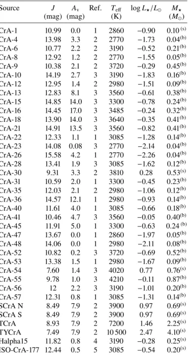
The basic stellar properties for the CrA sample are given in Table1, the distribution of SpTs is shown in Fig.2, while the mil-limeter observations, flux densities, and calculated disk masses are presented in Table3.
3. Observations
3.1. ALMA observations
We have carried out three executions of observations at 1.3 mm towards 43 Class II YSOs in the CrA molecular cloud using ALMA (2015.1.01058.S, PI: H. B. Liu). Each one of the 43 target sources was integrated for approximately 1 min in each epoch. The spectral setup consists of six spectral windows, of which the central frequency (GHz), total bandwidth (MHz), and fre-quency channel width (kHz) are (216.797, 1875, 488), (219.552, 59, 61), (219.941, 59, 61), (220.390, 117, 61), (230.531, 117, 31), and (231.484, 1875, 488), respectively. Additional observational details are summarized in Table2. The12CO (2–1),13CO (2–1), and C18O (2–1) transitions were also targeted with our spectral setup, but no clear detection was found because of strong fore-ground contamination. SO (6–5) and SiO (5–4) lines were also covered and not detected.
The data were manually calibrated using the CASA v5.1.1 software package (McMullin et al. 2007). The gain calibrator for the first epoch of observations was faint. To yield reasonably high signal-to-noise ratios (S/N) when deriving the gain phase solutions, the phase offsets among spectral windows were first solved using the passband calibration scan. After applying the phase offsets solution, the gain phase solution was then derived by combining all spectral windows. The calibration of the other two epochs of observations followed the standard procedure of ALMA quality assurance (i.e., QA2). The bootstrapped flux values of the calibrator quasar J1924-2914 were consistent with the SMA Calibrator list1 (Gurwell et al. 2007) to ∼10%. After
calibration, we fit the continuum baseline and subtract it from the spectral line data, using the CASA task uvcontsub.
The continuum data imaging was performed with multi-frequency synthesis (MFS) imaging of the continuum data using the CASA-clean task, and correcting for the primary beam. By jointly imaging all three epochs of data, for each target source field, the achieved continuum root-mean-square (RMS) noise level is ∼0.15 mJy beam−1, and the synthesized beam is θmaj× θmin= 0.0033 × 0.0031 (PA = 67◦), corresponding to a spatial resolution of ∼50 au at d = 154 pc. The imaged detections are presented in Fig.3.
It is important to note that because of an error when setting the observation coordinates, the decimal places of the target RAs have been trimmed: this results in an offset of the sources of up to 1500 east of the phase center: as a consequence, our images had to be primary beam corrected. The images in Fig. 3 have therefore been re-centered using the best-fit positions in Table3. 3.2. VLT/X-shooter observations
The spectroscopic follow-up observations for the 13 targets with missing SpT information were carried out in Pr.Id. 299.C-5048 (PI Manara) and Pr.Id. 0101.C-0893 (PI Cazzoletti) with the VLT/X-shooter spectrograph (Vernet et al. 2011). This
1 http://sma1.sma.hawaii.edu/callist/callist.html
Table 1. Stellar properties of the central sources of the disks in the sample.
2MASS ID Name RA Dec SpT Ref.
J18563974-3707205 CrA-1 18:56:39.76 −37:07:20.8 M6 1 J18595094-3706313 CrA-4 18:59:50.95 −37:06:31.6 M8 2 J19002906-3656036 CrA-6 19:00:29.07 −36:56:03.8 M4 3 J19004530-3711480 CrA-8 19:00:45.31 −37:11:48.2 M8.5 4 J19005804-3645048 CrA-9 19:00:58.05 −36:45:05.0 M1 3 J19005974-3647109 CrA-10 19:00:59.75 −36:47:11.2 M4 5 J19011629-3656282 CrA-12 19:01:16.29 −36:56:28.3 M5 6 J19011893-3658282 CrA-13 19:01:18.95 −36:58:28.4 M2 7 J19013232-3658030 CrA-15 19:01:32.31 −36:58:03.0 M3.5 7 J19013385-3657448 CrA-16 19:01:33.85 −36:57:44.9 M2.5 7 J19014041-3651422 CrA-18 19:01:40.41 −36:51:42.3 M1.5 7 J19015112-3654122 CrA-21 19:01:51.12 −36:54:12.4 M2 8 J19015180-3710478 CrA-22 19:01:51.86 −37:10:44.7 M4.5 1 J19015374-3700339 CrA-23 19:01:53.75 −37:00:33.9 M7.5 7 J19020682-3658411 CrA-26 19:02:06.80 −36:58:41.0 M7 1 J19021201-3703093 CrA-28 19:02:12.00 −37:03:09.4 M4.5 5 J19021464-3700328 CrA-29 19:02:14.63 −37:00:32.9 ... ... J19022708-3658132 CrA-30 19:02:27.07 −36:58:13.1 M0.5 5 J19023308-3658212 CrA-31 19:02:33.07 −36:58:21.2 M3.5 1 J19031185-3709020 CrA-35 19:03:11.84 −37:09:02.1 M5 3 J19032429-3715076 CrA-36 19:03:24.29 −37:15:07.7 M5 1 J19012576-3659191 CrA-40 19:01:25.75 −36:59:19.1 M4.5 1 J19014164-3659528 CrA-41 19:01:41.62 −36:59:52.7 M2 9 J19015037-3656390 CrA-42 19:01:50.48 −36:56:38.4 ... ... J19031609-3714080 CrA-45 E 19:03:16.09 −37:14:08.2 M3.5 1 J19031609-3714080 CrA-45 W 19:03:16.09 −37:14:08.2 M3.5 1 J18564024-3655203 CrA-47 18:56:40.28 −36:55:20.8 M6 1 J18570785-3654041 CrA-48 18:57:07.86 −36:54:04.4 M5 1 J19000157-3637054 CrA-52 19:00:01.58 −36:37:06.2 M1 10 J19011149-3645337 CrA-53 19:01:11.49 −36:45:33.8 M5 1 J19013912-3653292 CrA-54 19:01:39.15 −36:53:29.4 K7 9 J19015523-3723407 CrA-55 19:01:55.23 −37:23:41.0 K5 11 J19021667-3645493 CrA-56 19:02:16.66 −36:45:49.4 M4 4 J19032547-3655051 CrA-57 19:03:25.48 −36:55:05.3 M4.5 1 J19010860-3657200 SCrA N 19:01:08.62 −36:57:20 K3 6 J19010860-3657200 SCrA S 19:01:08.62 −36:57:20 M0 6 J19015878-3657498 TCrA 19:01:58.78 −36:57:49 F0 6 J19014081-3652337 TYCrA 19:01:40.83 −36:52:33.88 B9 6 J19041725-3659030 Halpha15 19:04:17.25 −36:59:03.0 M4 12 J19025464-3646191 ISO-CrA-177 19:02:54.65 −36:46:19.1 M4.5 4 ... G09-CrA-9 19:01:58.34 −37:01:06.0 ... ... J19015173-3655143 Haas17 19:01:51.74 −36:55:14.2 ... ... J19020410-3657013 IRS10 19:02:04.09 −36:57:01.2 ... ...
Notes.The RA and Dec in J2000 are from the Spitzer data presented in
Peterson et al.(2011).
References. (1) This work, (2)Bouy et al.(2004), (3)Romero et al. (2012), (4)López Martí et al.(2005), (5)Sicilia-Aguilar et al.(2011), (6) Forbrich & Preibisch (2007), (7) Sicilia-Aguilar et al. (2008), (8) Currie & Sicilia-Aguilar (2011), (9) Meyer & Wilking (2009), (10) Walter et al. (1997), (11) Herczeg & Hillenbrand (2014), (12)Patten(1998).
instrument covers the wavelength range from ∼300 to ∼2500 nm simultaneously, dividing the spectrum in three arms: the UVB (λλ ∼ 300–550 nm), the VIS (λλ ∼ 500–1050 nm), and the NIR (λλ ∼ 1000–2500 nm). All targets were observed both with a narrow slit – 1.000in the UVB, 0.900in the VIS, and NIR arms – leading to R ∼ 9000 and ∼10 000, respectively, and a wide slit
Table 2.ALMA observations towards Class II objects in the CrA molecular cloud.
Epoch 1 2 3
time (UTC; 2016) (Aug.01) 03:32-04:54 (Aug.01) 05:01-06:23 (Aug.02) 03:18-04:40
Project baseline lengths (min-max) (m) 14-1108 15-1075 15-1110
Absolute flux calibrator Pallas Pallas Pallas
Gain calibrator J1937-3958 J1924-2914 J1924-2914
Bootstrapped gain calibrator flux (Jy) 0.26 3.9 4.1
Passband calibration J1924-2914 J1924-2914 J1924-2914
Bootstrapped passband calibrator flux (Jy) 4.1 3.9 4.1
M0 M5 L0
K3
G8
G0
F0
A0
Spectral Type
0.00
0.05
0.10
0.15
0.20
U Sco
Lupus
CrA
Fig. 2. Distribution of the SpTs of the stars in CrA (Red) compared to
that of Lupus (Orange) and Upper Sco (Blue).
of 5.000used to obtain an accurate flux calibration of the spectra. The log of the observations is reported in TableB.2. The spec-tra of all the observed targets are detected in the NIR arm, while only five targets are bright enough and not too extinguished to be detected also in the UVB arm.
The reduction of the data was performed using the ESO X-shooter pipeline 2.9.3 (Modigliani et al. 2010). The pipeline performs the typical reduction steps, such as flat fielding, bias subtraction, order extraction and combination, rectification, wavelength calibration, and flux calibration using standard stars observed in the same night. We extracted the 1D spectra from the 2D images produced by the pipeline using IRAF and then removed telluric absorption lines in the VIS and NIR arms using telluric standard stars observed close in time and airmass (see e.g., Alcalá et al. 2014). The S/N of the spectra at different wavelengths is reported in TableB.2.
4. Results and analysis
4.1. Stellar properties
The SpTs for the targets were obtained from the literature (see Table1) or from the VLT/X-shooter spectra. The procedure used for the analysis of the X-shooter spectra was as follows. First, we corrected the spectra for extinction using the values from the literature (Dunham et al. 2015;Sicilia-Aguilar et al. 2008,2011) and the reddening law byCardelli et al.(1989) with RV= 3.1, as suggested bySicilia-Aguilar et al.(2008). We then calculated the values of a number of spectral indices both at wavelengths in the
VIS and the NIR arms, taken by those calibrated byRiddick et al. (2007),Jeffries et al.(2007), andHerczeg & Hillenbrand(2014), as inManara et al.(2017), and byTesti et al.(2001), as inManara et al.(2013). The SpTs derived from these indices are presented in TableB.1. The spectral indices in the VIS arms are more reli-able, and we select the SpT from these indices when available. The observed spectra along with a template of the relative SpTs are presented in Fig.B.1.
The SpTs are converted in effective temperatures (Teff) using the relation byHerczeg & Hillenbrand(2014). Stellar luminosity (L?) is obtained from the reddening-corrected J-band mag-nitudes and using the bolometric correction from Herczeg & Hillenbrand(2014), assuming for all targets the average distance of 154 pc calculated byDzib et al.(2018). With this information, we have been able to plot our data on the HR diagram (Fig.6) and to estimate the stellar masses (M?) for all the targets using the evolutionary tracks byBaraffe et al.(2015) for M?<1.4 M and Siess et al. (2000) for higher M? and ages younger than 1 Myr . The stellar parameters for the targets are reported in TableA.1.
4.2. Millimeter continuum emission
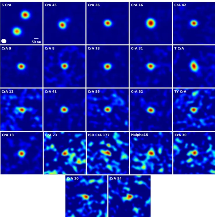
Among the 41 targets, 20 of them show a clear (≥4σ) detec-tion within a 100 radius from the nominal Spitzer location from Peterson et al. (2011). In addition, CrA-42 and T CrA show a ∼36σ and a ∼22σ detection, respectively, at a slightly larger dis-tance from their nominal Spitzer positions (100.05 for CrA-42 and 100.34 T CrA), and are also regarded as detections. The object S CrA is a known binary (Reipurth & Zinnecker 1993; Ghez et al. 1997; Takami et al. 2003), and we detected millimeter emission associated with both binary components. The object CrA-45 is also identified as a binary. The total number of detec-tions is therefore 24 out of the 43 targeted disks, and therefore the detection rate is ∼56%.
None of the disks show clear substructures, no transition disks with cavities with radii >25 au are found, and all of them appear to be unresolved or marginally resolved: a Gaussian is therefore fitted to the detected sources (two Gaussians for the binaries) in the image plane using the imfit task in CASA. The task returns the total flux-density F1.3 mm of the source along with the statistical uncertainty, the FWHM along the semi-major (amaj) and semi-minor (amin) axis, and the position angle (PA). The results of the fit are shown in Table32. The right ascension
(∆α) and declination (∆δ) offsets with respect to the Spitzer coor-dinates are also shown. The rms noise for the nondetections was calculated using the imstat task within a 100radius centered at
2 We note that the F1.3 mm uncertainty only includes the statistical
uncertainty from the fit, and not the 10% absolute flux calibration uncertainty.
50 au
Fig. 3.ALMA Band 6 1.3 mm continuum images of the 24 detections in CrA. The size of the images is 300× 300. The size of the beam is indicated
in the bottom-left corner of the first panel (000.31 × 000.33). The north of each image is upwards. The presented images have not been primary beam
corrected.
the Spitzer coordinates; for the detection, it was calculated in an annular region centered on the source and with inner and outer radii equal to 200and 400, respectively.
In order to constrain the average flux density of individ-ually undetected sources, a stacking analysis was also per-formed. The images were centered at their Spitzer coordinates (Table 1) and then stacked. Even after the stacking, no detec-tion was found and the average rms noise is 0.017 mJy beam−1, corresponding to a 3σ upper limit of 0.051 mJy assuming unresolved disks. However, it should be noted that the aver-age right ascension and declination offsets between the disks and the Spitzer positions, measured on the detections, are h∆αi = −0.1300 and h∆δi = 0.4700 respectively: it is therefore
possible that the undetected sources did not overlap during the stacking, and that the upper limit is actually higher than that quoted.
4.3. Dust masses
Assuming that the observed sub-millimeter emission is optically thin and isothermal, the relation between the emitting dust mass (Mdust) and the observed continuum flux at frequency ν (Fν) is as follows (Hildebrand 1983): Mdust= Fνd 2 κνBν(Tdust) ≈2.19 × 10 −6 d 160 !2 F1.3 mm(M ), (2)
Table 3.1.3 mm continuum properties of the sources targeted in our sample.
Name ∆α(a) ∆δ(a) F1.3 mm RMS amaj amin PA Mdust
(00) (00) (mJy) (mJy beam−1) (00) (00) (◦) (M⊕)
CrA-1 ... ... ... 0.10 ... ... ... ... CrA-4 ... ... ... 0.14 ... ... ... ... CrA-6 ... ... ... 0.08 ... ... ... ... CrA-8 −0.14 0.39 2.06 ± 0.17 0.16 0.365 ± 0.018 0.31 ± 0.014 81.90 ± 13.3 1.50 ± 0.12 CrA-9 −0.01 0.35 5.07 ± 0.16 0.33 0.389 ± 0.008 0.31 ± 0.005 81.07 ± 3.4 3.70 ± 0.12 CrA-10 0.07 0.34 0.65 ± 0.11 0.22 0.481 ± 0.119 0.25 ± 0.034 73.11 ± 7.9 0.48 ± 0.15 CrA-12 −0.05 0.42 1.37 ± 0.24 0.10 0.661 ± 0.100 0.32 ± 0.030 90.67 ± 4.8 1.00 ± 0.17 CrA-13 0.06 0.27 2.77 ± 0.26 0.21 0.367 ± 0.021 0.35 ± 0.019 126.02 ± 60.2 2.02 ± 0.19 CrA-15 ... ... ... 0.08 ... ... ... ... CrA-16 −0.23 0.45 20.34 ± 0.53 1.00 0.478 ± 0.008 0.44 ± 0.007 13.42 ± 11.5 14.84 ± 0.39 CrA-18 −0.20 0.52 5.36 ± 0.19 0.35 0.380 ± 0.008 0.32 ± 0.006 93.93 ± 5.3 3.92 ± 0.14 CrA-21 ... ... ... 0.08 ... ... ... ... CrA-22 ... ... ... 0.12 ... ... ... ... CrA-23 −0.26 0.76 0.35 ± 0.15 0.12 0.401 ± 0.120 0.28 ± 0.061 108.44 ± 24.8 0.26 ± 0.11 CrA-26 ... ... ... 0.11 ... ... ... ... CrA-28 ... ... ... 0.09 ... ... ... ... CrA-29 ... ... ... 0.11 ... ... ... ... CrA-30 −0.36 0.61 0.51 ± 0.18 0.09 0.504 ± 0.139 0.27 ± 0.046 96.59 ± 10.6 0.37 ± 0.13 CrA-31 −0.28 0.60 2.82 ± 0.19 0.19 0.416 ± 0.019 0.33 ± 0.013 80.58 ± 7.3 2.05 ± 0.14 CrA-35 ... ... ... 0.11 ... ... ... ... CrA-36 −0.14 0.38 12.9 ± 0.21 0.82 0.384 ± 0.004 0.32 ± 0.002 74.97 ± 2.1 9.41 ± 0.15 CrA-40 ... ... ... 0.11 ... ... ... ... CrA-41 −0.34 0.62 2.80 ± 0.19 0.21 0.384 ± 0.017 0.30 ± 0.011 85.01 ± 6.7 2.04 ± 0.14 CrA-42 −1.00 0.34 4.87 ± 0.21 0.34 0.377 ± 0.010 0.31 ± 0.007 81.88 ± 4.9 3.55 ± 0.16 CrA-45 E −0.36 0.63 29.82 ± 0.35 1.92 0.400 ± 0.003 0.34 ± 0.002 46.21 ± 1.7 21.76 ± 0.26 CrA-45 W 0.05 0.28 6.36 ± 0.34 1.92 0.393 ± 0.013 0.33 ± 0.009 87.43 ± 7.0 4.64 ± 0.25 CrA-47 ... ... ... 0.09 ... ... ... ... CrA-48 ... ... ... 0.12 ... ... ... ... CrA-52 0.05 −0.27 1.95 ± 0.17 0.16 0.404 ± 0.023 0.29 ± 0.012 70.00 ± 5.4 1.43 ± 0.12 CrA-53 ... ... ... 0.10 ... ... ... ... CrA-54 0.61 −0.14 0.48 ± 0.19 0.09 0.577 ± 0.189 0.26 ± 0.044 105.67 ± 7.8 0.35 ± 0.14 CrA-55 −0.26 0.24 0.81 ± 0.14 0.10 0.354 ± 0.037 0.29 ± 0.025 96.62 ± 19.4 0.59 ± 0.10 CrA-56 ... ... ... 0.10 ... ... ... ... CrA-57 ... ... ... 0.10 ... ... ... ... S CrA S −0.36 1.34 129.53 ± 2.09 10.4 0.451 ± 0.005 0.40 ± 0.004 75.03 ± 4.3 94.51 ± 1.52 S CrA N 0.23 0.13 140.30 ± 2.00 10.4 0.439 ± 0.004 0.39 ± 0.003 80.73 ± 3.7 102.36 ± 1.46 T CrA −0.06 1.34 4.99 ± 0.37 0.28 0.568 ± 0.033 0.37 ± 0.016 20.25 ± 4.3 3.64 ± 0.27 TY CrA 0.01 0.46 0.91 ± 0.18 0.13 0.362 ± 0.044 0.28 ± 0.026 90.13 ± 14.6 0.66 ± 0.13 IRS10 ... ... ... 0.08 ... ... ... ... Halpha15 −0.07 0.54 0.69 ± 0.22 0.08 0.529 ± 0.128 0.39 ± 0.078 142.60 ± 27.2 0.50 ± 0.16 ISO-CrA-177 −0.01 0.49 0.52 ± 0.17 0.11 0.535 ± 0.146 0.25 ± 0.037 71.91 ± 7.3 0.38 ± 0.13 Haas17 ... ... ... 0.11 ... ... ... ... G09-CrA-9 ... ... ... 0.09 ... ... ... ...
Notes. (a)Offset with respect to coordinates listed in Table1.
where d is the distance of the object, Fν is the measured flux-density, Bν(Tdust) is the Planck function for a given dust temperature Tdust, and κνis the dust opacity at frequency ν. To make the comparison with previous surveys easier, for the dust opacity κνwe follow the same approach ofAnsdell et al.(2016), assuming κν =10 cm2g−1 at 1000 GHz (Beckwith et al. 1990) and scaling it to our frequency using β = 1. The adopted value is therefore κν=2.3 cm2g−1 at ν = 230 GHz (1.3 mm). In the right-hand side of Eq. (2), the distance d is measured in parsecs and the flux density F1.3 mm is in millijanskys. For each object, the average distance of the cluster d = 154 pc was used. For the
dust temperature, we use a constant Tdust =20 K (Andrews & Williams 2005), rather than the Tdust =25 K × (L∗/L )0.25 rela-tion based on 2D continuum radiative transfer byAndrews et al. (2013) and used in other works (e.g.,Law et al. 2017). We adopt this simplified approach with a single grain opacity and temper-ature for all the disks in the sample following the approach of Ansdell et al.(2016) and to facilitate the comparison with other star-forming regions (see Sect.4.4). Moreover, it should be noted that no dependence of the average dust temperature on the stel-lar parameters was found with the more detailed modeling by Tazzari et al.(2017) for the Lupus disks.
Table 4.Global properties of the star-forming regions surveyed with ALMA in order of age.
Name Distance Age Average dust mass
(pc) (Myr) (M⊕) Taurus 129.5(1) 1–3 13 ± 2 Lupus 160(1), (a) 1–3 14 ± 3 CrA 154(1) 1–3 6 ± 3 Chameleon I 192(1) 2–3 24 ± 9 IC 348 321(1) 2–3 4 ± 1 σOri 388(1) 3–5 7 ± 1 Upper Sco 144(2) 5–10 5 ± 3
Notes.(a)The average distance of the 4 Lupus clouds was used. References. (1)Dzib et al.(2018); (2)de Zeeuw et al.(1999).
The dust masses of the disks in our sample are presented in Table3, along with the relative uncertainty calculated from the flux uncertainty. Only 3 disks out of 24 detections have a dust content ≥10 M⊕3 and are therefore large enough to form the core of a giant planet in the future. However, it is still pos-sible that a similar amount of dust mass is hidden in the inner disk regions due to very high optical depth (e.g.,Zhu et al. 2010; Liu et al. 2017;Vorobyov et al. 2018). We also note that very recent high-angular-resolution ALMA and VLA observations of disks are revealing that an important amount of dust is located in dense regions such as rings (e.g.,Andrews et al. 2018), which are optically thick at wavelengths around 1 mm (Dullemond et al. 2018). When optically thin emission is detected, higher masses are estimated (Carrasco-González et al. 2016).
The stacking of the nondetections gives an average 3σ upper limit corresponding to 0.036 M⊕, or about three lunar masses. 4.4. Comparison with other regions
The surveys of nearby star-forming regions over the last years have shown growing evidence of a decrease in the mass of the disks with age, reflecting dust growth and disk dispersal. Ansdell et al. (2016,2017) found consistent results, calculating the highest average mass in the youngest regions (1–3 Myr), and the lowest for the oldest Upper Sco association (5–10 Myr). The 2–3 Myr-old IC 348 is the only exception, showing an average dust mass of only 4 ± 1 M⊕(between the average σ Orionis and that of Upper Sco) despite its young age. This can be explained by the low-mass stellar population in the region (Ruíz-Rodríguez et al. 2018, also see Table4).
The same analysis was done here for CrA. The dust masses are uniformly calculated following the approach used byAnsdell et al.(2016), namely using Eq. (2) with the continuum fluxes (or the 3σ upper limits) from our ALMA data or from the literature, assuming a uniform T = 20 K, and inputting the frequency of the observation for each specific dataset. The distances assumed for each region are listed in Table4. For the Upper Sco region, only the disks classified as “full”, “evolved” and “transitional” from theBarenfeld et al.(2016) sample are included, while the “debris” and Class III YSOs, which likely represent a separate evolutionary stage, are excluded. Finally, in order to facilitate the comparison with the other samples, in this analysis we only
3 Five sources in total have a dust content ≥10 M
⊕if we also consider
CrA-16 and CrA-36, which have dust masses only marginally below 10 M⊕.
10
1
10
0
10
1
10
2
M
dust
[M ]
0.0
0.2
0.4
0.6
0.8
1.0
P
M
du
st
Cham I
Lupus
Ori
USco
CrA
Fig. 4. Comparison of the cumulative dust mass distributions of Lupus,
CrA, Cham I, σ Ori and Upper Sco, derived using a survival analysis accounting for the upper limits.
include the disks around stars with masses above the brown-dwarf limit (M? ≥ 0.1 M ). The Kaplan-Meier estimator from the lifelines4 and ASURV (Lavalley et al. 1992) packages
were then used to estimate the cumulative mass distribution and to calculate the average dust mass and its uncertainty while prop-erly accounting for the upper limits by using well-established techniques for left-censored data sets.
Figure4presents the results accounting for the upper limits given by the nondetections. With an average dust mass of 6 ± 3 M⊕, the distribution of the CrA disks appear closer to that of the old Upper Sco region rather than to those of the younger systems.
4.5. Mdisk–M?relation
A clear correlation between the dust mass of disks and the mass of the central star has been identified across all surveyed protoplanetary disk populations (Pascucci et al. 2016; Ansdell et al. 2017). This finding highlights how the disk properties are affected by the central star, and is consistent with the correla-tion between the frequency of giant planets and the masses of the host stars, both from observational and theoretical points of view (Alibert et al. 2011;Bonfils et al. 2013). Moreover, the slope of this relation has been observed to steepen with time, with the young Taurus, Lupus, and Chemeleon I regions (∼1–3 Myr) having slopes similar to each other and shallower than that found for the disks in the Upper Sco association (5–10 Myr).
Studying the Mdust− M? relation for the disks in the CrA sample provides useful information on the origin of the over-all low mass of the disk population found in Sect. 4.4. We derive the Mdust− M?relation using the same linear-regression Bayesian approach followed by Ansdell et al.(2017) and pre-sented byKelly(2007)5. Unlike other linear regression methods,
this approach is capable of simultaneously accounting for the uncertainties in both the measurements of Mdust and M?, of the intrinsic scatter of the data and of the disk nondetections, which result in upper limits on the disk masses. We note that the SpT, and therefore the stellar mass, is missing for five of our targets: for these objects the stellar mass is randomly drawn from the stellar mass distribution of the entire sample. In particular, four
4 10.5281/zenodo.1495175
0.1
1.0
M [M ]
0.1
1
10
100
1000
Flux at 150 pc [mJy]
USco Lupus CrAFig. 5. Correlation between dust disk flux scaled at 330 GHz (assuming
α =2.25, as inAnsdell et al. 2018) and at a distance of 150 pc with stellar mass for the objects in CrA. The slopes of Lupus and Upper Sco are also plotted for comparison. We show the results of the Bayesian fitting procedure byKelly (2007). The solid line represents the best-fit model, while the light lines show a subsample of models from the chains, giving an idea of the uncertainties.
of the objects with unknown SpT are also not detected with ALMA, while the other one (CrA-42) shows a clear detection of a disk at mm wavelengths. For the four nondetections, the stellar mass is therefore randomly drawn among the masses of the stars with nondetected disks, while the mass of CrA-42 is drawn from those showing a detection with ALMA. This uncer-tainty is also taken into account in the Bayesian approach we adopt by performing 100 different draws. In our fit, a standard uncertainty of 20% of M?on the stellar mass is assumed (Alcalá et al. 2017; Manara et al. 2017), while the uncertainties shown in Table 3were used for the Mdust values. Finally, it should be noted that only 1 out of 89 sources in Lupus was a Herbig Ae/Be star, while Upper Sco did not include any Herbig. We therefore decided not to include T CrA and TY CrA in the fit, for which the Mdust− M?relation might not hold.
The best-fit relation we find is then plotted in Fig.5in dark red, along with a subsample of all the models in the chains to show the uncertainty. As in the other surveys, we also find a cor-relation, where the best-fit model has a slope β = 2.32 ± 0.77 and intercept α = 1.29 ± 0.60. This regression intercept is lower that that of other regions, as a consequence of the low disk masses found in the region. The uncertainties of the best-fit parameters reflect the large scatter in the data and the low number statistics. In order to test that no strong bias was introduced by our pro-cedure, we also run the fit described above without any random draw, finding consistent results.
5. Discussion
5.1. Is CrA old?
The observed low dust masses of the disks suggest that the CrA objects targeted in our survey may have an age compa-rable to that of the Upper Sco association, rather than to the young Lupus region. Unlike CrA however, Upper Sco shows no presence of Class 0 or Class I sources, as expected for regions of 5–10 Myr old (Dunham et al. 2015). Moreover, most studies agree in assigning CrA an age of <3 Myr (e.g.,Meyer & Wilking 2009;Nisini et al. 2005;Sicilia-Aguilar et al. 2008,2011).
On the other hand, most of these studies focused only on the Coronet cluster, a small region extending ∼1 pc around the
3000
4000
5000
T
eff
[K]
3
2
1
0
1
lo
g
(L
*
/L
)
0.02 M 0.05 M 0.10 M 0.2 M 0.4 M 0.8 M 1.2 MCrA
CrA-XS
Lupus
Upper Sco
Fig. 6. HR diagram showing the sources in our CrA sample (red),
in the Lupus sample fromAnsdell et al. (2016) (orange), and in the Upper Sco sample (blue) fromBarenfeld et al.(2016). The evolution-ary tracks for different stellar masses and the relative isochrones from
Baraffe et al.(2015) are also plotted for reference. The isochrones refer (from top to bottom) to the 1, 2, 5, and 10 Myr isochrones. The colored solid lines show the approximate median value of the luminosity at each temperature.
R CrA YSO, and where most of the young embedded Class 0 and Class I sources are located (see Fig. 1). The hypothesis that the large-scale YSO population of the whole CrA cloud also includes a population of older objects therefore cannot be entirely ruled out. Some evidence of an additional older population has already been presented in previous studies. Neuhäuser et al. (2000) for example identify two classical T Tauri stars located outside the main cloud with an age of ∼10 Myr using ROSAT data. In addition,Peterson et al.(2011) perform a clustering analysis of the 116 YSOs in their sample, identifying a single core (corresponding to the Coronet) and a more extended population of PMS stars showing an age gradient west of the Coronet. They also observe that in the central core the ratio Class II/ Class I = 1.8, while the same ratio is Class II/ Class I = 2.3 when all the objects in the sample are considered, again hinting at a younger population inside the Coronet. Finally,Sicilia-Aguilar et al.(2011) point out that the relatively low disk fraction observed in the Coronet (∼50%López Martí et al. 2010, based on near IR photometry) is in strong contrast with the young age of the system: this inconsistency could be solved if an older population were also present. The large scatter in the Mdust− M? relation could also be a consequence of two stellar populations of different ages.
In order to further test if the Class II population in our sam-ple indeed includes an older population, we have placed them on the HR diagram using the SpTs listed in Table 1 and by deriving effective temperatures and bolometric corrections using the relationships inHerczeg & Hillenbrand(2014) and tables in Herczeg & Hillenbrand(2015), respectively. The obtained dia-gram is presented in Fig.6. For comparison, the Upper Sco and Lupus objects are also plotted. In contrast with what Fig.4 sug-gests, the HR diagram supports the scenario of a young CrA cluster with an age more consistent with that of Lupus than that of Upper Sco.
In order to make this conclusion evident, the median val-ues of the bolometric luminosities for each temperature are also shown (solid coloured lines in Fig. 6). The indicative age of the cluster is the isochrone closer to those median values: these
lines also suggest that CrA is younger than Upper Sco. However, a more extended spectral classification for a larger number of objects in CrA would be needed to fully test this older-population scenario.
5.2. Is CrA young?
If the whole CrA is coeval with an age of 1–3 Myr, some other mechanism has to be invoked to explain the low observed mm fluxes. For example, these fluxes could be due to low metallicity. However,James et al.(2006) determined metallicities for three T Tauri stars in CrA, finding them to be only slightly sub-solar, and not low enough to explain our observations.
External photo-evaporation is also known to play an impor-tant role in the disk mass evolution (Facchini et al. 2016;Winter et al. 2018a), and evidence of it occurring has been found in σ Ori (Maucó et al. 2016; Ansdell et al. 2017) where a clear corre-lation between disk mass and distance from the central Herbig O9V star has been observed, and in the Orion Nebula Cluster (Mann & Williams 2010;Eisner et al. 2018). However, in CrA no correlation between the mass of the disks (or the disk detection rate) and the distance from the brightest star (R CrA) is found. Moreover, in σ Ori external photo-evaporation has been shown to affect disks up to 2 pc away from the Herbig star, where the geometrically diluted far-ultraviolet (FUV) flux reached a value of ∼2000 G0. The SpT of R CrA is still uncertain, ranging from F5 (e.g.,Garcia Lopez et al. 2006) to B8 (e.g.,Hamaguchi et al. 2005). Even in the latter case, assuming a typical FUV lumi-nosity for a B8 star of LFUV ∼ 10 L (Antonellini et al. 2015) and accounting for geometric dilution, we find that the FUV flux would drop to ∼ 1 G0 in the first inner parsec from R CrA, thus ruling out external photo-evaporation as an explanation. Also, this calculation neglects dust absorption, which is probably very effective in the Coronet cluster around R CrA.
In view of the Mdisk− M?relation presented in Sect.4.5, it is also possible that a system dominated by low-mass stars shows a low-mass disk population, regardless of its age, as in the case of IC 348 (Ruíz-Rodríguez et al. 2018). It is therefore important, when comparing disk dust masses from different regions, to ver-ify that they have the same stellar mass distribution. In order to do this, we employ a Monte Carlo (MC) approach similar to that used byAndrews et al.(2013). We first normalize the stellar pop-ulations by defining stellar mass bins and randomly drawing the same number of sources in each bin from the reference sample (CrA) and from a comparison sample (Lupus, Chamaeleon I or Upper Sco). We then perform a two-sample logrank test for cen-sored datasets between the disk dust masses of the two samples to test the probability (pφvalue) that the two samples are randomly drawn from the same parent population. A low pφvalue indicates that the difference in disk masses cannot only be ascribed to dif-ferent stellar populations and that some other factor, such as disk evolution or the age of the system, must play a role. This pro-cess is repeated 10 000 times, and the results are used to create the cumulative distributions shown in Fig.7. When using Upper Sco as a comparison sample, we find a median pφvalue of 0.53, while the median pφfor Lupus is only 0.004. The conclusion is that even when accounting for the Mdust− M?relation, the disk dust mass distribution of CrA appears to be statistically differ-ent from that of Lupus, while it is significantly more similar to that of Upper Sco. Therefore, the comparably low masses of the protoplanetary disks in CrA cannot be explained in terms of low stellar masses.
Another way a disk can lose part of its mass is via tidal inter-action with other stars (e.g., Clarke & Pringle 1993; Pfalzner et al. 2005). This mechanism is however only effective in much
0.0001
0.001
0.01
0.1
1.0
p
0.0
0.2
0.4
0.6
0.8
1.0
f(
p
)
3
2
Upper Sco
Lupus
Fig. 7. Comparison of the mass distributions of Lupus and USco to that
of CrA, following the MC analysis proposed byAndrews et al.(2013). pφis the probability that the synthetic population drawn from the
com-parison sample (Lupus and Upper Sco) and the reference sample come from the same parent population. f (< pφ) is the cumulative distribution
for pφresulting from the logrank two-sample test for censored datasets
after 104MC iterations.
denser environments than CrA (e.g.,Winter et al. 2018b). In prin-ciple, it is possible to imagine that at very early stages most of the stars were located in a dense region (e.g., the Coronet) where they interacted violently before being ejected. However, the very low velocity dispersion of the stars in the cluster makes this sce-nario very unlikely (Neuhäuser et al. 2000). Tidal interaction can be effective in removing dust mass from a disk even in later stages when the disk is in a binary system (e.g.,Artymowicz & Lubow 1994), as was proposed byLong et al.(2018) to explain the low mm flux of some objects in Taurus. A higher-than-usual binary fraction could therefore explain the low disk masses observed in CrA. However, Ghez et al. (1997) show that the binary fraction of CrA is indistinguishable from those of Lupus and Chameleon I.
Finally, it is possible that the low mass distribution observed today is a consequence of a population of disks that has formed with a low mass from the very beginning. For example, the disk formation efficiency in a cloud with mass M0 depends on the sound speed cs and on the solid body rotation rate Ω0, where we have defined the disk-formation efficiency as the fraction of M0 that is in the disk at the end of the collapse stage, or as the ratio between Mdisk/M?at that time (Cassen & Moosman 1981; Terebey et al. 1984). In particular, clouds with higher csand Ω0 (i.e., warmer or more turbulent) will form more massive disks (also see Appendix A inVisser et al. 2009). Therefore, a cold parent cloud or one with low intrinsic angular momentum Ω0 will form disks with a lower mass and with a lower Mdisk/M?, as observed in CrA. Consistently, observations of dense cloud cores in the CrA cloud show line widths that are lower than in other regions (Tachihara et al. 2002). Moreover, because of the smaller circularization radius, the formed disks would also be smaller (e.g.,Dullemond et al. 2006) and potentially mostly optically thick, thus hiding an even larger fraction of the mass . Alternatively, small and optically thick disks could result from magnetic braking of the disks by means of the magnetic field threading the disk and the surrounding molecular cloud at the formation stage (e.g.,Mellon & Li 2008;Herczeg & Hillenbrand 2014;Krumholz et al. 2013). The same scenario was proposed by Maury et al.(2019) to explain the low occurrence of large (>60 AU) Class 0 disks in the CALYPSO sample.
Such scenarios, although not testable with the present data set, are consistent with the low disk mass distribution and with the low intercept of the Mdisk− M? in CrA and are not in con-tradiction with the young age of the stellar population. If the parent cloud initial conditions are indeed responsible for the low masses observed, this would be an additional critical aspect to be considered when studying planet formation and evolution. Since the conditions at the epoch of disk formation can be different in each star-forming region, proper modelling is required in order to ascertain the extent to which they can affect the initial disk mass distribution, the subsequent disk evolution, planet formation, and planetary populations.
Observationally, this could be tested by observing the mass of disks around Class 0 and Class I objects in CrA: if the disks are born with a low mass, the disk mass distribution even at these younger stages should be significantly lower than in other regions.
6. Conclusion
Here we present the first ALMA survey of 43 Class II protoplan-etary disks in the CrA nearby (d = 160 pc) star-forming region in order to measure their dust content and understand how it scales with the stellar properties. The ultimate goal was to test whether the relations found in other surveys between disk propertiesand age of the stellar population also hold for this region. The results presented here lead us to the following conclusions.
1. The average mm fluxes from the disks in CrA is low. This in turn converts into a low disk-mass distribution. Even though our observations are able to constrain dust masses down to ∼0.2 M⊕, the detection rate is only 56%. Moreover, we find that only three disks in our sample have a dust mass ≥10 M⊕ and thus sufficient mass to form giant planet cores.
2. We obtained VLT/X-shooter spectra for eight objects with previously unknown SpT, and derived their stellar physical properties.
3. Despite the apparent young age of the CrA stellar population, we find that the dust mass distribution of the disks in CrA is much lower than that of the young Lupus star-forming region which shares a similar age, while it appears to be consistent with that in the 5–10 Myr-old Upper Sco association. The correlation between disk dust mass Mdust and stellar mass M? previously identified in all other surveyed star-forming regions is confirmed. However, because of the low mass of the disks in our sample we find a much lower intercept. The large scatter of the data points does not allow the slope of the relation to be well constrained for CrA.
4. Since most of the age estimates of the CrA regions are based on the population of the compact Coronet cluster, a possible explanation for the low disk masses might be in principle that CrA also hosts an old population of disks, consistently with previous observations. The position of the objects of our sample on the HR diagram however seems to support the idea of a mostly coeval, young population.
5. Low disk masses in a young star-forming region can be explained by external photo-evaporation (as in the case of σOri) or by a low stellar mass population (as in IC 348). With our analysis, we can rule out both these scenarios for CrA. The stripping of material from the disks due to tidal interaction between different members of CrA or to close binaries can also be ruled out.
6. We suggest that initial conditions may play a crucial role in setting the initial disk mass distribution and its subsequent evolution. Small disks with low mass can originate from
a cloud with very low turbulence or sound speed, or can alternatively result from disk magnetic braking. It is there-fore important to better study the impact of initial conditions on the disk properties, especially if planet formation occurs even before 1 Myr age, as the recent results fromTychoniec et al.(2018) andManara et al.(2018) suggest.
Future surveys including younger Class 0 and I objects in CrA and other star-forming regions will help to test whether or not initial conditions play a critical role in shaping the physical properties of circumstellar disks.
Acknowledgements. We thank S. van Terwisga, S. Andrews, G. Lodato and A. Hacar for very useful discussions, and Dr. Mark Gurwell for compiling the SMA Calibrator List (http://sma1.sma.hawaii.edu/callist/callist.html).
We also acknowledge the DDT Committee and the Director of the La Silla and Paranal Observatory for granting DDT time. This work was partly sup-ported by the Italian Ministero dell’Istruzione, Università e Ricerca through the grant Progetti Premiali 2012 – iALMA (CUP C52I13000140001), by the Deutsche Forschungs-gemeinschaft (DFG, German Research Foundation) – Ref no. FOR 2634/1 TE 1024/1-1, and by the DFG cluster of excellence Ori-gin and Structure of the Universe (www.universe-cluster.de). This project
has received funding from the European Union’s Horizon 2020 research and innovation programme under the Marie Skłodowska-Curie grant agreement No 823823. H.B.L. is supported by the Ministry of Science and Technology (MoST) of Taiwan (Grant Nos. 108-2112-M-001-002-MY3 and 108-2923-M-001-006-MY3). J.M.A. acknowledges financial support from the project PRIN-INAF 2016 The Cradle of Life–GENESIS-SKA (General Conditions in Early Plane-tary Systems for the rise of life with SKA). C.F.M. and S.F. acknowledge an ESO Fellowship. M.T. has been supported by the DISCSIM project, grant agreement 341137 funded by the European Research Council under ERC-2013-ADG and by the UK Science and Technology research Council (STFC). Y.H. is supported by the Jet Propulsion Laboratory, California Institute of Technology, under a con-tract with the National Aeronautics and Space Administration. C.C.G and R.G.M acknowledge financial support from DGAPA UNAM. This paper makes use of the following ALMA data: ADS/JAO.ALMA#2015.1.01058.S. ALMA is a part-nership of ESO (representing its member states), NSF (USA) and NINS (Japan), together with NRC (Canada) and NSC and ASIAA (Taiwan), in cooperation with the Republic of Chile. The Joint ALMA Observatory is operated by ESO, AUI/NRAO and NAOJ. All the figures were generated with the python-based package matplotlib (Hunter 2007).
References
Alcalá, J. M., Natta, A., Manara, C. F., et al. 2014,A&A, 561, A2
Alcalá, J. M., Manara, C. F., Natta, A., et al. 2017,A&A, 600, A20
Alibert, Y., Mordasini, C., & Benz, W. 2011,A&A, 526, A63
Artymowicz, P., & Lubow, S. H. 1994,ApJ, 421, 651
Andrews, S. M., & Williams, J. P. 2005,ApJ, 631, 1134
Andrews, S. M., Wilner, D. J., Hughes, A. M., Qi, C., & Dullemond, C. P. 2009,
ApJ, 700, 1502
Andrews, S. M., Rosenfeld, K. A., Kraus, A. L., & Wilner, D. J. 2013,ApJ, 771, 129
Andrews, S. M., Huang, J., Pérez, L. M., et al. 2018,ApJ, 869, L41
Ansdell, M., Williams, J. P., van der Marel, N., et al. 2016,ApJ, 828, 46
Ansdell, M., Williams, J. P., Manara, C. F., et al. 2017,AJ, 153, 240
Ansdell, M., Williams, J. P., Trapman, L., et al. 2018,ApJ, 859, 21
Antonellini, S., Kamp, I., Riviere-Marichalar, P., et al. 2015,A&A, 582, A105
Baraffe, I., Homeier, D., Allard, F., & Chabrier, G. 2015,A&A, 577, A42
Barenfeld, S. A., Carpenter, J. M., Ricci, L., et al. 2016,ApJ, 827, 142
Beckwith, S. V. W., Sargent, A. I., Chini, R. S., & Guesten, R. 1990,AJ, 99, 924
Bell, C. P. M., Naylor, T., Mayne, N. J., et al. 2013,MNRAS, 434, 806
Benz, W., Ida, S., Alibert, Y., Lin, D., & Mordasini, C. 2014,Protostars and Planets VI(Tucson, AZ: University of Arizona Press), 691
Bonfils, X., Delfosse, X., Udry, S., et al. 2013,A&A, 549, A109
Bouy, H., Brandner, W., Martín, E. L., et al. 2004,A&A, 424, 213
Cardelli, J. A., Clayton, G. C., & Mathis, J. S. 1989,ApJ, 345, 245
Carmona, A., van den Ancker, M. E., & Henning, T. 2007,A&A, 464, 687
Carrasco-González, C., Henning, T., Chandler, C. J., et al. 2016,ApJ, 821, L16
Cassen, P., & Moosman, A. 1981,Icarus, 48, 353
Cieza, L. A., Ruíz-Rodríguez, D., Hales, A., et al. 2019,MNRAS, 482, 698
Clarke, C. J., & Pringle, J. E. 1993,MNRAS, 261, 190
Comerón, F. 2008,Handbook of Star Forming Regions, Volume II(San Fran-cisco: Astronomical Society of the Pacific), 5, 295
Cutri, R. M., Skrutskie, M. F., van Dyk, S., et al. 2003,VizieR Online Data Catalog: II/246
Deller, A. T., Forbrich, J., & Loinard, L. 2013,A&A, 552, A51
de Zeeuw, P. T., Hoogerwerf, R., de Bruijne, J. H. J., Brown, A. G. A., & Blaauw, A. 1999,AJ, 117, 354
Dullemond, C. P., Natta, A., & Testi, L. 2006,ApJ, 645, L69
Dullemond, C. P., Birnstiel, T., Huang, J., et al. 2018,ApJ, 869, L46
Dunham, M. M., Allen, L. E., Evans, N. J., II, et al. 2015,ApJS, 220, 11
Dzib, S. A., Loinard, L., Ortiz-León, G. N., Rodríguez, L. F., & Galli, P. A. B. 2018,ApJ, 867, 151
Eisner, J. A., Plambeck, R. L., Carpenter, J. M., et al. 2008,ApJ, 683, 304
Eisner, J. A., Arce, H. G., Ballering, N. P., et al. 2018,ApJ, 860, 77
Evans, N. J., II, Dunham, M. M., Jørgensen, J. K., et al. 2009,ApJS, 181, 321
Facchini, S., Clarke, C. J., & Bisbas, T. G. 2016,MNRAS, 457, 3593
Fedele, D., van den Ancker, M. E., Henning, T., et al. 2010,A&A, 510, A72
Forbrich, J., & Preibisch, T. 2007,A&A, 475, 959
Gaia Collaboration (Prusti, T., et al.) 2016,A&A, 595, A1
Gaia Collaboration (Brown, A. G. A., et al.) 2018,A&A, 616, A1
Galván-Madrid, R., Liu, H. B., Manara, C. F., et al. 2014,A&A, 570, L9
Garcia Lopez, R., Natta, A., Testi, L., & Habart, E. 2006,A&A, 459, 837
Ghez, A. M., McCarthy, D. W., Patience, J. L., & Beck, T. L. 1997,ApJ, 481, 378
Gurwell, M. A., Peck, A. B., Hostler, S. R., Darrah, M. R., & Katz, C. A. 2007, From Z-Machines to ALMA: (Sub)Millimeter Spectroscopy of Galaxies,ASP Conf. Ser., 375, 234
Haisch, K. E., Jr., Lada, E. A., & Lada, C. J. 2001,ApJ, 553, L153
Hennebelle, P., & Ciardi, A. 2009,A&A, 506, L29
Herczeg, G. J., & Hillenbrand, L. A. 2014,ApJ, 786, 97
Herczeg, G. J., & Hillenbrand, L. A. 2015,ApJ, 808, 23
Hernández, J., Hartmann, L., Megeath, T., et al. 2007,ApJ, 662, 1067
Hildebrand, R. H. 1983,QJRAS, 24, 267
Hamaguchi, K., Yamauchi, S., & Koyama, K. 2005,ApJ, 618, 360
Hunter, J. D. 2007,Comput. Sci. Eng., 9, 3
James, D. J., Melo, C., Santos, N. C., & Bouvier, J. 2006,A&A, 446, 971
Jeffries, R. D., Oliveira, J. M., Naylor, T., Mayne, N. J., & Littlefair, S. P. 2007,
MNRAS, 376, 580
Kelly, B. C. 2007,ApJ, 665, 1489
Kenyon, S. J., Gómez, M., & Whitney, B. A. 2008,Handbook of Star Forming Regions, Volume I(San Francisco: ASP), 4, 405
Krumholz, M. R., Crutcher, R. M., & Hull, C. L. H. 2013,ApJ, 767, L11
Lavalley, M., Isobe, T., & Feigelson, E. 1992, Astronomical Data Analysis Software and Systems I,ASP Conf. Ser., 25, 245
Law, C. J., Ricci, L., Andrews, S. M., Wilner, D. J., & Qi, C. 2017,AJ, 154, 255
Luhman, K. L. 2008, Handbook of Star Forming Regions, Volume II (San Francisco: ASP), 5, 169
Liu, H. B., Galván-Madrid, R., Forbrich, J., et al. 2014,ApJ, 780, 155
Liu, H. B., Vorobyov, E. I., Dong, R., et al. 2017,A&A, 602, A19
Lindegren, L., Hernandez, J., Bombrun, A., et al. 2018,A&A, 616, A2
Long, F., Pinilla, P., Herczeg, G. J., et al. 2018,ApJ, 869, 17
López Martí, B., Eislöffel, J., & Mundt, R. 2005,A&A, 444, 175
López Martí, B., Spezzi, L., Merín, B., et al. 2010,A&A, 515, A31
Luri, X., Brown, A. G. A., Sarro, L. M., et al. 2018,A&A, 616, A9
Manara, C. F., Testi, L., Rigliaco, E., et al. 2013,A&A, 551, A107
Manara, C. F., Testi, L., Herczeg, G. J., et al. 2017,A&A, 604, A127
Manara, C. F., Morbidelli, A., & Guillot, T. 2018,A&A, 618, L3
Mann, R. K., & Williams, J. P. 2010,ApJ, 725, 430
Maucó, K., Hernández, J., Calvet, N., et al. 2016,ApJ, 829, 38
Maury, A. J., André, P., Testi, L., et al. 2019,A&A, 621, A76
McMullin, J. P., Waters, B., Schiebel, D., Young, W., & Golap, K. 2007, Astro-nomical Data Analysis Software and Systems XVI,ASP Conf. Ser., 376, 127
Mellon, R. R., & Li, Z.-Y. 2008,ApJ, 681, 1356
Meyer, M. R., & Wilking, B. A. 2009,PASP, 121, 350
Morbidelli, A., & Raymond, S. N. 2016,J. Geophys. Res. Planets, 121, 1962
Mordasini, C., Alibert, Y., Benz, W., et al. 2012,A&A, 541, A97
Modigliani, A., Goldoni, P., Royer, F., et al. 2010,Proc. SPIE, 7737, 773728
Neuhäuser, R., & Forbrich, J. 2008,Handbook of Star Forming Regions, Volume II(San Francisco: ASP), 5, 735
Neuhäuser, R., Walter, F. M., Covino, E., et al. 2000,A&AS, 146, 323
Nisini, B., Antoniucci, S., Giannini, T., & Lorenzetti, D. 2005,A&A, 429, 543
Ortiz-León, G. N., Loinard, L., Kounkel, M. A., et al. 2017,ApJ, 834, 141
Pascucci, I., Testi, L., Herczeg, G. J., et al. 2016,ApJ, 831, 125
Patten, B. M. 1998, Cool Stars, Stellar Systems, and the Sun,ASP Conf. Ser., 154, 1755
Peterson, D. E., Caratti o Garatti, A., Bourke, T. L., et al. 2011,ApJS, 194, 43
Pfalzner, S., Vogel, P., Scharwächter, J., & Olczak, C. 2005,A&A, 437, 967
Reipurth, B., & Zinnecker, H. 1993,A&A, 278, 81
Riddick, F. C., Roche, P. F., & Lucas, P. W. 2007,MNRAS, 381, 1067
Romero, G. A., Schreiber, M. R., Cieza, L. A., et al. 2012,ApJ, 749, 79
Ruíz-Rodríguez, D., Cieza, L. A., Williams, J. P., et al. 2018,MNRAS, 478, 3674
Schaefer, G. H., Hummel, C. A., Gies, D. R., et al. 2016,AJ, 152, 213
Sicilia-Aguilar, A., Henning, T., Juhász, A., et al. 2008,ApJ, 687, 1145
Sicilia-Aguilar, A., Henning, T., Kainulainen, J., & Roccatagliata, V. 2011,ApJ, 736, 137
Siess, L., Dufour, E., & Forestini, M. 2000,A&A, 358, 593
Tachihara, K., Onishi, T., Mizuno, A., & Fukui, Y. 2002,A&A, 385, 909
Takami, M., Bailey, J., & Chrysostomou, A. 2003,A&A, 397, 675
Tazzari, M., Testi, L., Natta, A., et al. 2017,A&A, 606, A88
Terebey, S., Shu, F. H., & Cassen, P. 1984,ApJ, 286, 529
Testi, L., D’Antona, F., Ghinassi, F., et al. 2001,ApJ, 552, L147
Testi, L., Natta, A., Scholz, A., et al. 2016,A&A, 593, A111
Tychoniec, Ł., Tobin, J. J., Karska, A., et al. 2018,ApJS, 238, 19
Vernet, J., Dekker, H., D’Odorico, S., et al. 2011,A&A, 536, A105
Visser, R., van Dishoeck, E. F., Doty, S. D., & Dullemond, C. P. 2009,A&A, 495, 881
Vorobyov, E. I., Akimkin, V., Stoyanovskaya, O., Pavlyuchenkov, Y., & Liu, H. B. 2018,A&A, 614, A98
Walter, F. M., Vrba, F. J., Wolk, S. J., Mathieu, R. D., & Neuhauser, R. 1997,AJ, 114, 1544
Winter, A. J., Clarke, C. J., Rosotti, G., et al. 2018a,MNRAS, 478, 2700
Winter, A. J., Clarke, C. J., Rosotti, G., & Booth, R. A. 2018b,MNRAS, 475, 2314
Zhu, Z., Hartmann, L., & Gammie, C. 2010,ApJ, 713, 1143
1 Max-Planck-Institute for Extraterrestrial Physics (MPE),
Giessen-bachstr. 1, 85748 Garching, Germany e-mail: [email protected]
2 European Southern Observatory (ESO), Karl-Schwarzschild-Str. 2,
85748 Garching, Germany
3 Academia Sinica Institute of Astronomy and Astrophysics,
Roo-sevelt Rd, Taipei 10617, Taiwan
4 Leiden Observatory, Leiden University, Niels Bohrweg 2, 2333 CA
Leiden, The Netherlands
5 INAF – Osservatorio Astronomico di Capodimonte, Via Moiariello
16, 80131 Napoli, Italy
6 Center for Integrative Planetary Science, University of California at
Berkeley, Berkeley, CA 94720, USA
7 Department of Astronomy, University of California at Berkeley,
Berkeley, CA 94720, USA
8 Institute for Astronomy, University of Hawai‘i at M¯anoa, Honolulu,
HI 96822, USA
9 Instituto de Radioastronomía y Astrofísica (IRyA-UNAM),
Univer-sidad Nacional Autónoma de México, Campus Morelia, Apartado Postal 3-72, 58090 Morelia, Michoacán, Mexico
10 Department of Physics & Astronomy, University of Victoria,
Victoria, BC, V8P 1A1, Canada
11 Centre for Astrophysics Research, University of Hertfordshire,
Col-lege Lane, Hatfield AL10 9AB, UK
12 Harvard-Smithsonian Center for Astrophysics, 60 Garden St,
Cambridge, MA 02138, USA
13 National Astronomical Observatory of Japan, 2-21-1 Osawa,
Mitaka, Tokyo 181-8588, Japan
14 Anton Pannekoek Institute for Astronomy, University of Amsterdam,
PO Box 94249, 1090 GE, Amsterdam, The Netherlands
15 Jet Propulsion Laboratory, California Institute of Technology,
Pasadena, CA 91109, USA
16 Division of Liberal Arts, Kogakuin University, 1-24-2
Nishi-Shinjuku, Shinjuku-ku, Tokyo 163-8677, Japan
17 Department of Astronomy/Steward Observatory, The University of
Arizona, 933 North Cherry Avenue, Tucson, AZ 85721, USA
18 Department of Astronomy, The University of Tokyo, 7-3-1, Hongo,
Bunkyo-ku, Tokyo 113-0033, Japan
19 Astrobiology Center of NINS, 2-21-1, Osawa, Mitaka, Tokyo
181-8588, Japan
20 Institute of Astronomy, University of Cambridge, Madingley Road,
Cambridge CB3 0HA, UK
21 Homer L. Dodge Department of Physics and Astronomy, University
Appendix A: Additional stellar properties
TableA.1shows a compilation of the most relevant stellar param-eters used in our analysis. The J magnitude is taken from the 2MASS survey (Cutri et al. 2003). The extinctions are either derived from our VLT/X-shooter spectra or from the references in Col. 4. We note that the extinctions fromDunham et al.(2015) were not derived from the stellar spectra but from extinction maps and might therefore systematically overestimate the real extinction towards the star by 1–2 mag (see Sect. 4.1 inPeterson et al. 2011). In order to make sure that the extinction values from Dunham et al.(2015) were accurate, we compared them to those derived from the spectra bySicilia-Aguilar et al.(2011) for eight targets common to the two samples. We found that the extinc-tions derived with the two methods are consistent within the uncertainties. The effective temperatures and bolometric lumi-nosities were derived as explained in Sect.5.1and then used to determine the stellar masses as explained in Sect.4.1.
Table A.1.Compilation of the most relevant stellar properties used in our analysis.
Source J Av Ref. Teff log L?/L M?
(mag) (mag) (K) (M ) CrA-1 10.99 0.0 1 2860 −0.90 0.10(s) CrA-4 13.98 3.3 2 2770 −1.73 0.04(b) CrA-6 10.77 2.2 2 3190 −0.52 0.21(b) CrA-8 12.92 1.2 2 2770 −1.55 0.05(b) CrA-9 10.38 2.1 2 3720 −0.29 0.45(b) CrA-10 14.19 2.7 3 3190 −1.83 0.16(b) CrA-12 12.95 1.4 2 2980 −1.51 0.09(b) CrA-13 12.83 8.1 3 3560 −0.61 0.38(b) CrA-15 14.85 14.0 3 3300 −0.78 0.24(b) CrA-16 14.45 17.0 3 3485 −0.24 0.32(b) CrA-18 13.90 14.0 3 3640 −0.35 0.41(b) CrA-21 14.91 13.5 3 3560 −0.82 0.41(b) CrA-22 12.33 1.1 1 3085 −1.28 0.14(b) CrA-23 14.08 0.08 3 2770 −2.14 0.04(b) CrA-26 15.58 4.2 1 2770 −2.26 0.04(b) CrA-28 13.41 1.9 3 3085 −1.62 0.12(b) CrA-30 9.31 3.3 2 3810 0.28 0.53(s) CrA-31 10.59 2.0 1 3300 −0.45 0.23(b) CrA-35 12.03 2.1 2 2980 −1.06 0.12(b) CrA-36 14.57 12.1 1 2980 −0.93 0.14(b) CrA-40 11.61 4.0 1 3085 −0.66 0.18(b) CrA-41 10.46 4.7 3 3560 −0.05 0.40(b) CrA-45 11.91 5.0 1 3300 −0.63 0.24(b) CrA-47 13.67 0.0 1 2860 −1.97 0.05(b) CrA-48 14.06 0.0 1 2980 −2.11 0.08(b) CrA-52 10.82 0.2 3 3720 −0.69 0.52(b) CrA-53 13.38 1.5 1 2980 −1.67 0.09(b) CrA-54 7.60 1.4 3 4020 0.77 0.76(s) CrA-55 9.78 1.0 3 4210 −0.11 0.87(b) CrA-56 12 2.2 3 3190 −1.01 0.20(b) CrA-57 12.31 0.8 1 3085 −1.31 0.14(b) SCrA N 8.49 7.9 2 3900 0.97 0.69(s) SCrA S 8.49 7.9 2 3900 0.97 0.69(s) TCrA 8.93 7.9 2 7200 1.46 2.25(s) TYCrA 7.49 7.9 2 10 500 2.47 4.10(s) Halpha15 11.82 0.8 4 3190 −0.28 0.25(s) ISO-CrA-177 12.44 0.5 5 3085 −0.54 0.20(s)
Notes.Only the stars with known SpT were included.
References. (1) This work; (2)Dunham et al.(2015); (3)Sicilia-Aguilar
et al.(2011); (4)Patten(1998); (5)López Martí et al.(2005); (s)Siess et al.(2000); (b)Baraffe et al.(2015).
Appendix B: VLT/X-shooter spectra
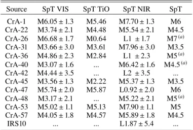
In this section we present the VLT/X-shooter spectra obtained and presented in Fig.B.1. The SpTs derived from the different spectral indices calibrated are presented in TableB.1. In particu-lar, SpT VIS was obtained from the average values fromRiddick et al. (2007), as in Manara et al. (2013, 2017); SpT TiO was obtained with the index byJeffries et al.(2007); SpT NIR was obtained with the indices byTesti et al. (2001), as in Manara et al.(2013); and the uncertainties represent the spread between the different indices in the VIS and NIR arms. The adopted SpTs reported in the last column of TableB.1are taken from the indices calculated in the VIS arm of the spectrum. In addition, the log of our X-shooter observations is presented in TableB.2 along with the S/N achieved at different wavelengths.
Table B.2.Night log and basic information on the spectra.
Source Date of observation (UT) Exp. time (Nexp× s) Slit width (00) S/N at λ (nm) Hα Li
UVB VIS NIR UVB VIS NIR 400 700 1000
Pr.Id. 299.C-5048 (PI Manara)
CrA-31 2017-09-01T03:30:30.048 4 × 215 4 × 135 4 × 3 × 75 1.0 0.9 0.9 8 20 21 Y Y
CrA-36 2017-09-17T02:22:50.221 4 × 600 4 × 690 4 × 3 × 250 1.0 0.9 0.9 0 0 23 Y N
CrA-42 2017-09-09T02:14:39.978 4 × 630 4 × 700 4 × 3 × 250 1.0 0.9 0.9 0 0 1 N N
CrA-45 2017-09-06T00:37:53.044 4 × 440 4 × 340 4 × 3 × 150 1.0 0.9 0.9 0 24 1110 Y Y
Pr.Id. 0101.C-0893 (PI Cazzoletti)
CrA-1 2018-05-28T04:25:20.708 4 × 90 4 × 150 4 × 150 1.0 0.9 0.9 24 14 35 Y Y CrA-22 2018-06-14T06:36:52.359 4 × 190 4 × 250 4 × 250 1.0 0.9 0.9 3 20 58 Y ... CrA-26 2018-06-12T05:54:41.945 4 × 190 4 × 250 4 × 250 1.0 0.9 0.9 0 2 13 Y N CrA-40 2018-05-26T08:08:42.457 4 × 190 4 × 250 4 × 250 1.0 0.9 0.9 1 56 69 Y Y CrA-47 2018-06-15T04:01:23.919 4 × 190 4 × 250 4 × 250 1.0 0.9 0.9 1 13 309 Y Y CrA-48 2018-05-26T05:05:48.019 4 × 190 4 × 250 4 × 250 1.0 0.9 0.9 11 21 20 Y N CrA-53 2018-05-26T06:41:48.012 4 × 190 4 × 250 4 × 250 1.0 0.9 0.9 1 14 52 Y Y CrA-57 2018-05-27T05:18:45.651 4 × 90 4 × 150 4 × 150 1.0 0.9 0.9 3 17 83 Y Y IRS10 2018-06-11T06:08:20.787 4 × 190 4 × 250 4 × 250 1.0 0.9 0.9 0 0 2 N N
Notes.Column 1 contains the name of the source, Col. 2 the date and time of the observations, Cols. 3–5 the exposure times, Cols. 6–8 the slit widths, Cols. 9–11 the S/N measured at the indicated wavelengths, and Cols. 12 and 13 indicate whether or not the Hαand Li lines have been
detected.
Table B.1.Spectral types derived from different spectral indices.
Source SpT VIS SpT TiO SpT NIR SpT
CrA-1 M6.05 ± 1.3 M5.46 M7.70 ± 1.3 M6 CrA-22 M3.74 ± 2.1 M4.48 M5.54 ± 2.1 M4.5 CrA-26 M6.68 ± 1.7 M0.64 L1 ± 1.7 M7(a) CrA-31 M3.66 ± 3.0 M3.61 M7.96 ± 3.0 M3.5 CrA-36 M4.86 ± 2.3 M2.84 L1 ± 2.3 M5(a) CrA-40 M3.07 ± 1.6 ... M6.42 ± 1.6 M4.5(a) CrA-42 M4.44 ± 3.5 ... L2 ± 3.5 ... CrA-45 M3.56 ± 1.3 M2.22 M5.37 ± 1.3 M3.5 CrA-47 M5.74 ± 2.0 M5.87 L0.92 ± 2.0 M6 CrA-48 M3.17 ± 2.1 ... M5.22 ± 2.1 M5(a) CrA-53 M5.02 ± 1.1 M5.13 M7.90 ± 1.1 M5 CrA-57 M4.05 ± 1.8 M4.57 M5.89 ± 1.8 M4.5 IRS10 ... ... L1.87 ± 5.4 ...
1000
Wavelength [nm]
10
18
10
16
10
14
Fl
ux
[e
rg
s
1
cm
2
nm
1
]
CrA1
1000
Wavelength [nm]
10
19
10
17
10
15
10
13
Fl
ux
[e
rg
s
1
cm
2
nm
1
]
CrA22
1000
Wavelength [nm]
10
19
10
16
10
13
Fl
ux
[e
rg
s
1
cm
2
nm
1
]
CrA26
Fig. B.1.Spectra observed in our X-shooter programs (black) along with a template with the same SpT (red). The names of the sources are in the