Discovering Exceptional Individuals and Properties in Data

(1)

U

NIVERSITÀ DELLA

C

ALABRIA

Dipartimento di Elettronica,

Informatica e Sistemistica

Dottorato di Ricerca in

Ingegneria dei Sistemi e Informatica

XX ciclo

Tesi di Dottorato

Discovering Exceptional Individuals

and Properties in Data

(2)

(3)

UNIVERSITÀ DELLA

CALABRIA

Dipartimento di Elettronica,

Informatica e Sistemistica

Dottorato di Ricerca in

Ingegneria dei Sistemi e Informatica

XX

ciclo

Tesi

di

Dottorato

Discovering Exceptional Individuals

and Properties in

Data

Fabio Fassetti

Coordinatore

Prof. Domenico Talia

Supervisori

(4)

DEIS – Dipartimento di Elettronica, Informatica e Sistemistica Novembre 2007

(5)

Acknowledgments

I wish to gratefully acknowledge my Ph.D. supervisor Luigi Palopoli for his teachings and for having provided me with ideas and suggestions; my super-visor Fabrizio Angiulli for having been a guidance for me, for his encourage-ments and for his support as a friend. I want to thank my Ph.D. coordinator, Domenico Talia, and all the colleagues I worked with during these years, for many valuable comments and stimulating discussions. My deepest gratitude goes to my family and to all my friends for their help, their unlimited support in any difficult time and for making pleasant my days.

(6)

(7)

List of Figures

3.1 The DOLPHIN distance-based outlier detection algorithm. . . 26

3.2 Analysis of the algorithm. . . 29

3.3 Course of the size of INDEX. . . 35

3.4 Execution time and effectiveness of pruning rules. . . 36

3.5 Sensitivity to parameters R and k. . . 37

3.6 Comparison with other methods. . . 38

4.1 Exact data stream distance-based outlier detection algorithm. . . 44

4.2 Approximate data stream distance-based outlier detection algorithm. . . 45

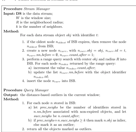
4.3 Precision and Recall of approx-STORM. . . 54

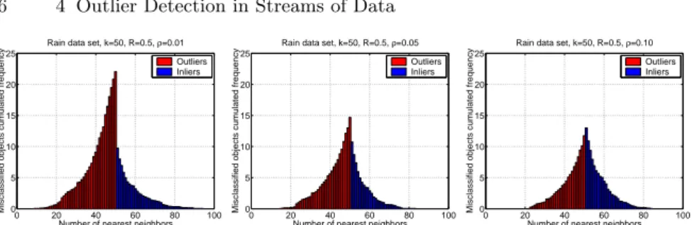
4.4 Number of nearest neighbors associated with the misclassified objects of the Rain data set. . . 56

5.1 Zoo database (A=hair, B=feathers, C=eggs, D=milk, E=airborne, F=aquatic, G=predator, H=toothed, I=backbone, J=breathes, K=venomous, L=fins, M=legs (set of values: 0,2,4,5,6,8), N=tail, O=domestic, P=catsize, Q=type (integer values in range [1,7])). . . 63

5.2 Example Database . . . 70

5.3 Histograms of the example data base. . . 71

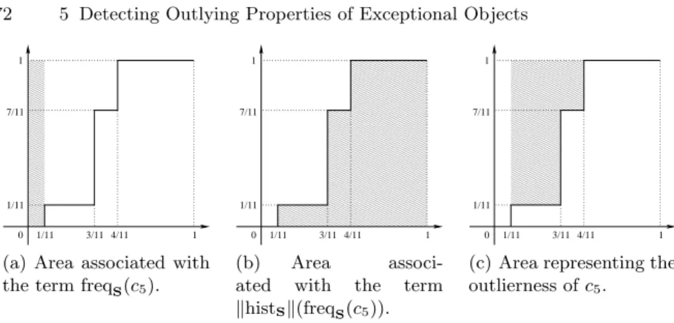
5.4 The areas associated with the curve of the cumulated frequency histogram. . . 72

5.5 Example of outlierness computation. . . 73

5.6 Example of Dataset with Functional Dependencies . . . 75

5.7 An example of the reduction used in Theorem 3 . . . 79

5.8 Example of reduction used in Theorem 4 . . . 81

5.9 Example of upper bounds obtained on the database DBex_{. . . 94}

5.10 The algorithm FindOutliers. . . 97

5.11 The algorithm FindLocalOutliers. . . 98

(10)

2 List of Figures

5.13 Index structure . . . 102

5.14 Example of frequency histogram management. . . 104

5.15 Explanation tree example. . . 106

5.16 Experimental results on the synthetical data set family. . . 108

5.17 Mean number of node visited (starting from the top of each figure the curves are for σ = 0.25, 0.5, 0.75, and 1.0). Notice that, on the Voting records database, curves for σ = 0.75 and σ = 1.0 overlap. . . 109

(11)

List of Tables

3.1 Experiments on a massive dataset. . . 39 4.1 Elaboration time per single object [msec]. . . 57 5.1 Computational complexity results concerning the outlying

property detection problem. . . 87 5.2 Breast cancer data: attribute domains. . . 113 5.3 Random dataset family: experimental results. . . 114

(12)

(13)

List Of Publications

Fabio Fassetti, Gianluigi Greco and Giorgio Terracina. Efficient discovery of loosely structured motifs in biological data. In Proceedings of the 2006 ACM Symposium on Applied Computing(SAC), pages 151–155, 2006.

Fabrizio Angiulli, Fabio Fassetti and Luigi Palopoli. Un metodo per la scoperta di propriet`a inattese. In Proceedings of the Fourteenth Italian Symposium on Advanced Database Systems (SEBD), pages 321–328, 2006.

Fabio Fassetti, Gianluigi Greco and Giorgio Terracina. L-SME: A Tool for the Efficient Discovery of Loosely Structured Motifs in Biological Data. In Proceedings of the Fifteenth Italian Symposium on Advanced Database Systems (SEBD), pages 389–396, 2007.

Fabio Fassetti and Bettina Fazzinga. FOX: Inference of Approximate Func-tional Dependencies from XML Data. In Proceedings of Eighteenth Inter-national Workshop on Database and Expert Systems Applications (DEXA), pages 10–14, 2007.

Fabio Fassetti and Bettina Fazzinga. Approximate Functional Dependencies for XML Data. In Local Proceedings of Eleventh East-European Conference on Advances in Databases and Information Systems (ADBIS), pages 86–95,2007. Fabrizio Angiulli and Fabio Fassetti. Very Efficient Mining of Distance-Based Outlier. In Proceedings of the 2007 ACM CIKM International Conference on Information and Knowledge Management, pages 791–800, 2007.

Fabrizio Angiulli and Fabio Fassetti. Detecting Distance-Based Outliers in Streams of Data. In Proceedings of the 2007 ACM CIKM International Con-ference on Information and Knowledge Management, pages 811–820, 2007. Fabrizio Angiulli, Fabio Fassetti and Luigi Palopoli. Detecting Outlying Prop-erties of Exceptional Objects.Submitted to an international journal, 2007. Fabio Fassetti, Gianluigi Greco and Giorgio Terracina. Mining Loosely Struc-tured Motifs from Biological Data. Submitted to an international journal, 2007.

(14)

(15)

1 Introduction

This thesis aims at providing novel techniques and methods in the complex scenario of knowledge discovery. This research field can be defined as “the nontrivial extraction of implicit, previously unknown, and potentially useful information from data”, and it has witnessed increasing interest in the last few years and a lot of research efforts have been spent on related problems. Knowledge discovery tasks mainly belong to four general categories:

1. dependency inference 2. class identification 3. class description 4. outlier detection

The former three categories focus on the search of characteristics applicable to a large percentage of objects. Many data mining tasks belong to these categories as association rules, classification and data clustering. Conversely, the fourth category deals with a very small percentage of dataset objects, which are often regarded as noise. Nevertheless, “one person’s noise may be another person’s signal”. Indeed, in a lot of real world domains, an object that, for some reasons, is different from the majority of the population which it belongs to, is the real interesting knowledge to be inferred from the population. Think, for example, an anomalous traffic pattern in a computer network that could signal the presence of an hacked computer. Similarly, anomalies in credit card transaction data could represent an illegal action, or in monitoring athlete performances, the detection of data which do not conform to expected normal behavior, is the main issue. Many clustering, classification, and dependency detection methods produce outliers as a by-product of their main task. For example, in classification, mislabeled objects are considered outliers and thus they are removed from the training set to improve the accuracy of the resulting classifier, while, in clustering, objects that do not strongly belong to any cluster are considered outliers. Nevertheless, searching for outliers through techniques specifically designed for tasks different from outlier detection could not be advantageous. As an example, clusters can be distorted by outliers

(16)

8 1 Introduction

and, thus, the quality of the outliers returned is affected by their presence. Moreover, other than returning a solution of higher quality, outlier detection algorithms can be vastly more efficient than non ad-hoc algorithms.

The design of novel and efficient outlier detection techniques is the field in which the first part of this thesis aims to provide novel contributions. Here, the discovery of exceptionalities is tackled by considering a classical setting.

On the contrary, the second part of the thesis is concerned with a novel data mining task related to abnormality search. In classical meaning, outlier detection consists of mining objects which are anomalous, for some reasons, with respect to the population which they belong to. Conversely, here the anomalous object is known in advance and the goal is to find the features it posses that can justify its exceptionality. In more details, it is assumed that you are given a significantly large data population characterized by a certain number of attributes, and you are provided with the information that one of the individuals in that data population is abnormal, but no reason whatso-ever is given to you as to why this particular individual is to be considered abnormal. The interest here is precisely to single out such reasons.

This thesis is organized as follows. In the following of this chapter some data mining concepts and issues are briefly surveyed. Particular attention is dedicated to outlier detection tasks, introducing the basic terminology and some problems that arise in this scenario. Finally, the main contribution of the thesis are presented.

The remainder of the thesis is divided in two parts. The first one regards the detection of anomalous objects in a given population. In particular, ter 2 introduces the outlier detection problem and surveys related work; Chap-ter 3 presents a novel efficient technique for mining outlier objects coming from huge disk-resident data sets. The statistical foundation of the efficiency of the proposed method is investigated. An algorithm, called DOLPHIN, is presented and its performance and its complexity are described. Finally, the results of a large experimental campaign are reported in order to show the behavior of DOLPHIN on both synthetic and real data cases. Furthermore, comparisons with existing methods have been conducted, showing DOLPHIN to outper-form the current state-of-the-art algorithms. Chapter 4 presents a method to detect outliers in streams of data, namely, when data objects are continuously delivered. Two algorithms are presented. The first one exactly answers outlier queries, but has larger space requirements. The second algorithm is directly derived from the exact one, has limited memory requirements and returns an approximate answer based on accurate estimations with a statistical guaran-tee. Several experiments have been accomplished, confirming the effectiveness of the proposed approach and the high quality of approximate solutions.

The second part of the thesis is concerned with the problem of discovering sets of attributes that account for the (a-priori stated) abnormality of an in-dividual within a given data population. A criterion is presented to measure the abnormality of combinations of attribute values featured by the given

(17)

ab-1.1 Overview on Exceptional Object Discovery 9

normal individual with respect to the reference population. The problem of individuating abnormal properties is formally stated and analyzed, and the in-volved computational complexity is discussed. Such a formal characterization is then exploited in order to devise efficient algorithms for detecting outlying properties. Experimental evidence, which is also accounted for, shows that the algorithms are able to mine meaningful information and to accomplish the computational task by examining a negligible fraction of the search space.

1.1 Overview on Exceptional Object Discovery

In exceptional object discovery, the purpose is to find the objects that are dif-ferent from most of the other objects. These objects are referred to as outliers. In many applications, singling out exceptional objects is much more interest-ing than detectinterest-ing common characteristics. For example, consider fraud de-tection, commerce monitoring, athlete performances, and so on. Traditionally, the goal of the outlier detection task is to find outliers in a given population; nevertheless, there are many other emerging applications, such as network flow monitoring, telecommunications, data management, etc., in which the data set is not given, but data arrive continuously and it is either unnecessary or impractical to store all incoming objects. In this context, a hard challenge becomes that of finding the most exceptional objects in the data stream. In the following of this chapter, some preliminary concepts about both outlier detection and data streams are presented.

1.1.1 Outlier Detection

Outlier Detection aims at singling out exceptional objects. A natural ques-tion arises, that is: “What is an excepques-tional object (an outlier)?”. Although there is not a formal and general definition of an outlier, the Hawkins’ def-inition well capture the essence of an outlier: “an outlier is an observation that deviates so much from other observations as to arouse suspicions that it was generated by a different mechanism”[Hawkins, 1980]. Former works in outlier detection rely on statistics, and more than one hundred discordancy tests have been developed to identify outliers. Nevertheless, this kind of ap-proach is not generally applicable either because there may not be a suitable test for a distribution or because no known distribution suitably models the data. Moreover, since in the data mining context data distribution is almost always unknown, a suitable standard distribution modeling data has to be inferred from data and the cost of this operation is often high, especially for large dataset. Thus, in recent years, numerous efforts have been made in this outstanding context to overcome these shortcomings.

Proposed approaches to outlier detection can be mainly classified in super-vised, semi-supersuper-vised, and unsupervised. In supervised methods, an already

(18)

10 1 Introduction

classified data set is available and it is employed as training set. The ob-jects belonging to it are already known to be normal or abnormal, and they are exploited to learn a model to correctly classify any other object. In semi-supervised methods, instead, only a set of normal objects is given and available as the training set. The aim of this methods is to find a rule to partition the object space into regions, an accepting region and a rejecting one. The for-mer contains the normal objects, whereas the latter contains the objects that significantly deviate from the training set. Finally, in unsupervised methods, no training set is given and the goal of finding outliers in a given data set is pursued by computing a score for each object suited to reflect its degree of abnormality. These scores are usually based on the comparison between an object and its neighborhood.

Data mining researchers have largely focused on unsupervised approaches. These approaches can be mainly further classified in deviation-based [Arning et al., 1996], density-based [Breunig et al., 2000], MDEF-based [Papadimitriou et al., 2003], and distance-based [Knorr and Ng, 1998].

Deviation-based techniques [Arning et al., 1996] identify as exceptional the subset Ixof the overall data set I whose removal maximizes the similarity

among the objects in I\Ix.

Density-based methods, introduced in [Breunig et al., 2000], are based on the notion of local outlier. Informally, the Local Outlier Factor (LOF) measures the outlierness degree of an object by comparing the density in its neighborhood with the average density in the neighborhood of its neighbors. The density of an object is related to the distance to its kth_{nearest neighbor.}

Density-based methods are useful when the data set is composed of subpop-ulations with markedly different characteristics.

The multi-granularity deviation factor (MDEF), introduced in [Papadim-itriou et al., 2003], is similar to the LOF score, but the neighborhood of an object consists of the objects within an user-provided radius and the den-sity of an object is defined on the basis of the number of objects lying in its neighborhood.

Distance-based outlier detection has been introduced by Knorr and Ng [1998] to overcome the limitations of statistical methods, this novel notion of outliers, is a very general one and is not based on statistical considerations. They define outliers as follows:

Definition 1. Let DB be a set of objects, k a positive integer, and R a positive real number. An object o of DB is a distance-based outlier (or, simply, an outlier) if less than k objects in DB lie within distance R from o.

The term DB(k, R)−outlier is a shorthand for Distance-Based outlier de-tected using parameters k and R. Objects lying at distance not greater than R from o are called neighbors of o. The object o is considered a neighbor of itself.

This definition is very intuitive since it defines an outlier as an object lying distant from others dataset objects.

(19)

1.1 Overview on Exceptional Object Discovery 11

Moreover, Definition 1 is a solid one, since it generalizes many notions of outliers defined in statistics for standard distributions and supported by statis-tical outlier tests. In other words, for almost all discordancy tests, if an object o is an outlier according to a specific test, then o is also a DB(k, R)−outlier for suitable values of parameters k and R. Nevertheless, this definition can not replace all statistical outlier tests. For example, if no distance can be defined between dataset objects, DB-outlier notion cannot be employed.

Some variants of the original definition have been subsequently introduced in the literature. In the previous one, the number of DB-outliers is not fixed. In some applications can be useful to find the top − n outliers, namely the n outliers scoring the highest score of abnormality. Then, a score function able to rank outliers is needed. In particular, in order to rank the outliers, Ramaswamy et al. [2000] introduced the following definition:

Definition 2. Given two integers k and n, an object o is an outlier if less than n objects have higher value for Dk _{than o, where D}k _{denotes the distance of}

the kth _{nearest neighbor of the object.}

Subsequently, Angiulli and Pizzuti [2002], with the aim of taking into account the whole neighborhood of the objects, proposed to rank them on the basis of the sum of the distances from the k nearest neighbors, rather than considering solely the distance to the kth_{nearest neighbor. Therefore, they introduced the}

following definition:

Definition 3. Given two integers k and n, an object is an outlier if less than n objects have higher value for wk, where wk denotes the sum of the distances

between the object and its k nearest neighbors Last definition was also used by Eskin et al. [2002].

The three definitions above are closely related to one another. In particular, there exist values for the parameters such that the outliers found by using the first definition are the same as those obtained by using the second definition, but not the third one. In this work we will deal with the original definition provided by Knorr and Ng [1998], even if we will compare also with approaches following the definition given by Ramaswamy et al. [2000].

1.1.2 Anomalies in Streams of Data

A data stream is a large volume of data coming as an unbounded sequence where, typically, older data objects are less significant than more recent ones. This is because the characteristics of the data may change over time, and then the most recent behavior should be given larger weight.

Therefore, data mining on evolving data streams is often performed based on certain time intervals, called windows. Two main different data streams window models have been introduced in literature: landmark window and sliding window [Golab and ¨Ozsu, 2003].

(20)

12 1 Introduction

In the first model, some time points (called landmarks) are identified in the data stream, and analysis are performed only for the stream portion which falls between the last landmark and the current time. Then, the window is identified by a fixed endpoint and a moving endpoint.

In contrast, in the sliding window model, the window is identified by two sliding endpoints. In this approach, old data points are thrown out as new points arrive. In particular, a decay function is defined, that determines the weight of each point as a function of elapsed time since the point was observed. A meaningful decay function is the step function. Let W be a parameter defining the window size and let t denote the current time, the step function evaluates to 1 in the temporal interval [t − W + 1, t], and 0 elsewhere.

In all window models the main task is to analyze the portion of the stream within the current window, in order to mine data stream properties or to single out objects conforming with characteristics of interest.

Due to the intrinsic characteristics of a data stream, and in particular since it is neverending, finding outliers in a stream of data becomes a hard challenge.

1.2 Overview on Exceptional Property Discovery

The anomaly detection issues introduced in the previous two sections is a prominent research topic in data mining, as the numerous proposed ap-proaches witness. A lot of efforts have been paid to discover unexpected ele-ments in data populations and several techniques have been presented [Tan et al., 2005].

The classical problem in outlier detection is to identify anomalous objects in a given population. But, what does the term anomalous mean? When an object can be defined anomalous? As discussed in the previous section, there are many definition to establish the exceptionality of an object. An object is identified as outlier if it possesses some characteristics, established by the chosen definition, that the other dataset objects do not possess, or if it does not posses some characteristics that the other dataset objects posses. Hence, in words, the characteristics distinguishing inliers from outliers are a-priori chosen, and then, outliers are detected according to the choice. Nevertheless, in many real situations, a novel but related problem arises, which is someway the inverse of the previous one: it is a-priori known which objects are inliers and which ones are outliers and the characteristics distinguishing them have to be detected. A limited attention has been paid till now to this problem. This problem has many practical applications. For instance, in analyzing health parameters of a sick patient, if a history of healthy patients is given and if the same set of parameters is available, then it is relevant to single out that subset of those parameters that mostly differentiate the sick patient from the healthy population. As another example, the history of the characteristics athlete that has established an exceptional performance can be analyzed to

(21)

1.2 Overview on Exceptional Property Discovery 13

detect those characteristics distinguishing the last exceptional performance from the previous ones.

Hence, in this context, a population is given. It can consist of entries re-ferred to the same individual (performance history of an athlete) or to different individuals (sick and healthy patients), and for each entry several attributes are stored. The outlier is known and the goal is to single out properties it posses, that justify its abnormality. Often, such properties are subsets of at-tribute values featured by the given outlier, that are anomalous with respect to the population the outlier belongs to. Naturally, the following question arises: what does the term anomalous mean? When a property can be defined anomalous? Also in this context, a lot of definitions can be introduced. For example, a property can be defined as anomalous, if it is different from the rest of the population, and this difference is statistically significative. Moreover, different definitions characterize properties referred to numerical attributes and properties referred to categorical attribute. For example, for numerical attributes a distance among properties can be defined, while for categorical attributes the frequency of a property can be meaningful.

(22)

(23)

Part I

(24)

(25)

2 The Outlier Detection Problem

2.1 Introduction

In this part of the thesis, the outlier detection problem is addressed. In par-ticular, two scenarios are considered. In the first one, outliers have to be discovered in disk-resident data sets. These data sets can be accessed many times, even if they are assumed to be very large and then the cost to be spent to read them from disk is relevant. In the second scenario considered in this thesis, data are assumed to come continuously from a given data source. Thus, they can be read only once, and this adds further difficulties and novel constraints to be taken in account.

There exist several approaches to the problem of singling out the objects mostly deviating from a given collection of data [Barnett and Lewis, 1994, Arning et al., 1996, Knorr and Ng, 1998, Breunig et al., 2000, Aggarwal and Yu, 2001, Jin et al., 2001, Papadimitriou et al., 2003]. In particular, distance-based approaches [Knorr and Ng, 1998] exploit the availability of a distance function relating each pair of objects of the collection. These approaches iden-tify as outliers the objects lying in the most sparse regions of the feature space. Distance-based definitions [Knorr and Ng, 1998, Ramaswamy et al., 2000, Angiulli and Pizzuti, 2002] represent an useful tool for data analysis [Knorr and Ng, 1999, Eskin et al., 2002, Lazarevic et al., 2003]. They have robust theoretical foundations, since they generalize diverse statistical tests. Further-more, these definitions are computationally efficient, as distance-based outlier scores are monotonic non-increasing with the portion of the database already explored.

In recent years, several clever algorithms have been proposed to fast detect distance-based outliers [Knorr et al., 2000, Ramaswamy et al., 2000, Bay and Schwabacher, 2003, Angiulli and Pizzuti, 2005, Ghoting et al., 2006, Tao et al., 2006]. Some of them are very efficient in terms of CPU cost, while some others are mainly focused on minimizing the I/O cost. Nevertheless, it is worth to

(26)

18 2 The Outlier Detection Problem

notice that none of them is able to simultaneously achieve the two previously mentioned goals when the dataset does not fit in main memory.

In this thesis a novel technique for mining distance-based outliers in an high dimensional very large disk-resident dataset, with both near linear CPU and I/O cost, is presented.

The proposed algorithm, DOLPHIN, performs only two sequential scans of the data. It needs to maintain in main memory a subset of the dataset and employs it as a summary of the objects already seen. This subset allows to efficiently search for neighbors of data set objects and, thus, to fast determine whether an object is an inlier or not. An important feature of the method is that memory-resident data is indexed by using a suitable proximity search approach. Furthermore, DOLPHIN exploits some effective pruning rules to early detect inliers, without needing to find k neighbors for each of them. Importantly, both theoretical justifications and empirical evidences that the amount of main memory required by DOLPHIN is only a small fraction of the dataset are provided. Therefore, the approach is feasible on very large disk-resident datasets.

The I/O cost of DOLPHIN corresponds to the cost of sequentially reading two times the input dataset file. This cost is negligible even for very large datasets. As for the CPU cost, the algorithm performs in quadratic time but with a little multiplicative constant, due to the introduced optimizations. In practice, the algorithm needs to compute only a little fraction of the overall number of distances (which is quadratic with respect to the size of the data set) in order to accomplish its task. DOLPHIN has been compared with state of the art methods, showing that it outperforms existing ones of at least one order of magnitude.

As previously stated, in the data stream context, new challenges arise along with the outlier detection problems. First of all, data come continuously. Second, with each data stream object, a life time is associated. While in data sets each object is equally relevant, in data streams an objects expires after some periods of time, namely, it is no more relevant in the analysis. Third, the characteristics of the stream, and then the characteristics of the relevant population may change during time.

In this thesis, a contribution in a data stream setting is given. Specifically, the problem of outlier detection adopting the sliding window model with the step function as the decay function is addressed.

The proposed approach introduces a novel concept of querying for outliers. Specifically, previous work deals with continuous queries, that are queries eval-uated continuously as data stream objects arrive; conversely, here, one-time queries are considered. This kind of queries are evaluated once over a point-in-time (for a survey on data streams query models refer to [Babcock et al., 2002]). The underlying intuition is that, due to stream evolution, object prop-erties can change over time and, hence, evaluating an object for outlierness when it arrives, although meaningful, can be reductive in some contexts and

(27)

2.1 Introduction 19

sometimes misleading. On the contrary, by classifying single objects when a data analysis is required, data concept drift typical of streams can be cap-tured. To this aim, it is needed to support queries at arbitrary points-in-time, called query times, which classify the whole population in the current window instead of the single incoming data stream object.

The example below shows how concept drift can affect the outlierness of data stream objects.

Example 1. Consider the following figure.

o1 t2 t1 t3 t4 t5 t6 t7 value o2 o3 R R o7 o5 o4 o6 time o9 t2 t1 t3 t4 t5t6 t7 t8 t9 t10 t11 t12 value o12 R R time o6 o11 o10 o1 o3 o5 o4 o2 o7 o8

The two diagrams represent the evolution of a data stream of 1-dimensional objects. The abscissa reports the time of arrival of the objects, while the ordinate reports the value assumed by each object. Let the number k of nearest neighbors to consider be equal to 3, and let the window size W be equal to 7. The dashed line represents the current window.

The left diagram reports the current window at time t7 (comprehending

the interval [t1, t7]), whereas the right diagram reports the current window at

time t12(comprehending the interval [t6, t12]).

First of all, consider the diagram on the left. Due to the data distribution in the current window at time t7, the object o7 is an inlier, since it has four

neighbors in the window. Then, if an analysis were required at time t7, the

object o7 would be recognized as an inlier. Note that o7 belongs to a very

dense region.

Nevertheless, when stream evolves the data distribution change. The re-gion, which o7 belongs to, becomes sparse, and data stream objects assume

lower values. The right figure shows the evolution of the stream until time t12.

In the novel distribution, o7 has not any neighbor. Then, if an analysis were

required at time instant t12, o7should be recognized as an outlier. Note that

(28)

2.2 Related Work

Distance-based outliers have been first introduced by Knorr and Ng [1998], which also presented the early three algorithms to detect distance-based out-liers. The first one is a block nested loop algorithm that runs in O(dN2_{) time,}

where N is the number of objects and d the dimensionality of the data set. It extends the na¨ıve nested loop algorithm by adopting a strategy to reduce the number of data blocks to be read from the disk. This kind of approach has a quadratic cost with respect to N , that can be impractical for handling large data sets.

The second and the third one are two cell-based algorithms, which are linear with respect to N , but exponential in d. Then, they are fast only if d is small. In particular, the former is designed to work with memory-resident data sets, whereas the latter deals with disk-resident ones and, then, aims at minimizing the number of passes over the data sets (indeed it guarantees at most three passes over the data sets). Basically, the main idea of cell-based algorithms is to partition the space into cells of length R

2√d, and counting

the number of objects within cells. The number of neighbors of an object can be determined by examining only the cells close to the cell which the object belongs to.

A shortcoming of this technique is that the number of cells is exponential with respect to the number of dimensions d.

Therefore, the latter kind of techniques is impractical if d is not small, and the former approach does not scale well w.r.t. N ; then, efforts for develop-ing efficient algorithms scaldevelop-ing well to large datasets have been subsequently made.

Ramaswamy et al. [2000] present two novel algorithms to detect outliers. The first assumes the dataset to be stored in a spatial index, like the R∗_-tree

[Beckmann et al., 1990], and uses it to compute the distance of each dataset object from its kth _{nearest neighbor. Pruning optimizations to reduce the}

number of distance computations while querying the index are exploited. The authors noted that this method is computationally expensive and introduced a partition-based algorithm to reduce the computational cost. The second algorithm first partitions the input points using a clustering algorithm, and then prunes the partitions that cannot contain outliers. Experiments were reported only up to ten dimensions.

Bay and Schwabacher [2003] introduce the distance-based outlier detec-tion algorithm ORCA. Basically, ORCA enhances the naive block nested loop algorithm with a simple pruning rule and randomization, obtaining a near lin-ear scaling on large and high dimensional data sets. The major merit of this work is to show that the CPU time of the their schema is often approximately linear in the dataset size.

In order to improve performances of ORCA, Ghoting et al. [2006] propose the algorithm RBRP (Recursive Binning and Re-Projection). The method has two phases. During the first phase, a divisive hierarchical clustering algorithm

(29)

2.2 Related Work 21

is used to partition objects into bins, i.e. group of objects likely to be close to each other. Then, objects in the same bin are reorganized according to the projection along the principal component. During the second phase, the strategy of ORCA is employed on the clustered data, obtaining improved performances.

Recently, Tao et al. [2006] point out that for typical values of the parame-ters, ORCA has quadratic I/O cost. Then, they present an algorithm, named SNIF (for ScaN with prIoritized Flushing), intended to work with datasets that do not fit into main memory, and whose major goal is to achieve linear I/O cost. They propose two algorithms, the first one retrieves the outliers by scanning the dataset three times but has smaller space requirements, the second algorithm needs to perform in some cases only two data set scans, but has larger space requirements. Roughly speaking, the first algorithm initially accommodates in memory a sample set of objects of fixed size s and then counts and stores the number of neighbors within distance R

2 of these objects

by scanning the data set. Using the stored information, during a second scan, some objects are recognized as inliers, and all the other objects are stored in memory.

The authors show that, in practice, the total amount of memory required is smaller than the available memory. Then, they propose a second algorithm, which stores much more objects in memory, in order to reduce the proba-bility of the third scan. In particular, dataset objects, and for each of them the number of neighbors found till now, are stored. Whenever the available memory gets full, the algorithm halves the occupied memory, by discarding recognized inliers and by storing objects with lower priority in a verification file. The priority is the probability that the object is an outlier. Next, a sec-ond scan is performed to classify the objects in memory and the objects of the verification file that are loaded in memory. If the memory becomes full before the verification file is exhausted, then the second scan is performed to empty the memory and a third scan is required for the remaining verification file objects. Authors show that, in practice, the verification file contains a very small number of objects and in some cases is empty, then SNIF needs only two scans to accomplish its task. Furthermore, authors show that the I/O cost of their algorithm is low and insensitive to the parameters, but time performances of the method were not deeply investigated.

The HilOut algorithm, [Angiulli and Pizzuti, 2005], detects the top distance-based outliers, according to the weight score, in a numerical data sets. It makes use of the Hilbert space-filling curve in order to linearize the data set and con-sists of two phases: the first phase guarantees at least an approximate solution, by scanning at most d+1 times the data set and with temporal cost quadratic in d and linear in N , where d is the number of dimensions of the data set and N is the number of data set objects. If needed, the second phase is performed. It provides the exact solution after a second data set scan examining the can-didates outlier returned by the first phase. Experimental results show that the

(30)

algorithm always stops, reporting the exact solution, during the first phase after much less than d + 1 steps.

In domains where distance computations are very expensive, e.g. the edit distance between subsequences or the quadratic distance between image color histograms, determining the exact solution may become prohibitive. Wu and Jermaine [2006] considered this scenario and describe a sampling algorithm for detecting distance-based outliers with accuracy guarantees. Roughly speaking, the algorithm works as follows. For each data point, α points are randomly sampled from the data set. Using the user-specified distance function, the kth_{-N N distance of the data set objects in those α samples are computed.}

When the data set objects end, the sampling algorithm returns the objects whose sampled kth_{-N N distance is the greatest. The total number of}

com-puted distances is αN , where N is the number of data set objects. Authors analyze the statistical properties of the proposed algorithm to provide accu-racy guarantees thereof.

This thesis presents a novel distance-based outlier detection algorithm, named DOLPHIN (for Detecting OutLiers PusHing data into an INdex), whose goal is to achieve both near linear CPU and I/O cost on very large disk-resident datasets, with a small usage of main memory. It gains efficiency by integrating pruning rules and state of the art database index technologies. It must be preliminary noted that none of the existing methods is able to achieve both these goals. Some algorithms exploit indexing or clustering [Ramaswamy et al., 2000, Ghoting et al., 2006], but require to build the in-dex, or to perform clustering, on the whole dataset, and, in some cases, to store the clustered data in main memory. On the other hand, the technique of detecting outliers by directly exploiting existing indexing techniques [Bentley, 1975, Beckmann et al., 1990, Berchtold et al., 1996, B¨ohm et al., 2001, Ch´avez et al., 2001] in order to search for the kth_{nearest neighbor of an object, suffers}

of the drawback that all the dataset objects have to be stored into the index structure. Besides, note that the approach of computing the k nearest neigh-bors of each object is not very efficient for outlier detection, since, for a lot of objects, this task can be avoided by using clever algorithms. Furthermore, the approach in [Bay and Schwabacher, 2003] works directly on disk-resident data and is efficient in CPU time, being able to achieve roughly near linear time for some combinations of the parameters but, as pointed out by Tao et al. [2006], its I/O cost may be quadratic. On the other hand, the approach in [Tao et al., 2006] keeps low the I/O cost, but it is not as efficient from the point of view of the CPU cost (for example, note that, SNIF compares each dataset object to all the s centroids, but s = 1,000, or greater, is a typical value for this parameter), and cannot be used in nonmetric spaces.

DOLPHIN detects outliers in disk-resident datasets. It performs two se-quential scans of input dataset file. During the first scan, it maintains a data structure storing a small subset of the dataset objects in main memory, to-gether with some additional information. This memory-resident data structure represents a summary of the already seen objects, and it is used to determine

(31)

2.2 Related Work 23

whether the object currently read from disk is an inlier or not. If it can-not be determined that the current object is an inlier, then it is added to the memory-resident data. At the same time, objects already stored in main memory could be recognized as inliers and may be discarded. By retaining a moderate fraction of proved inliers, DOLPHIN is able to effectively exploit the triangular inequality to early prune inliers, without the need of computing k distances per object.

Outlier detection methods previously discussed are designed to work in a batch framework, namely under the assumption that the whole data set is stored in secondary memory and multiple passes over the data can be accom-plished. Hence, they are not suitable for the online paradigm or for processing data streams. While the majority of the approaches to detect anomalies in data mining consider the batch framework, some researchers have attempted to address the problem of online outlier detection. In [Yamanishi et al., 2000], the SmartSifter system is presented, addressing the problem from the view-point of statistical learning theory. The system employs an online discounting learning algorithm to learn a probabilistic model representing the data source. An important feature of the employed algorithm is that it discounts the effect of past data in the on-line process by means of a decay function. It assigns a score to the datum, measuring how large the model has changed after learning. Every time a datum is input, SmartSifter updates the model and assigns a score to the input datum on the basis of the model. In particular, SmartSifter measures how large the model updated with the new datum has moved from the one learned before. The algorithm returns ad outliers the data having high scores, that have, then, an high probability of being statistical outliers.

In [Ghoting et al., 2004], authors present LOADED (Link-based Outlier and Anomaly Detectin in Evolving Data Sets), an algorithm for outlier de-tection in evolving data sets. The authors focus on two main aspects: first, their algorithm accomplishes only one-pass over the data set and, then, it is employable for on-the-fly outlier detection; second, their algorithm deals with both categorical and continuous attributes. In particular, authors define a metric that is able to determine dependencies between both categorical and continuous attributes. As for categorical attributes, they define that there is a link between two objects if they have a pair attribute-value in common. The strength of the link between two objects is the number of links they posses. Conversely, for continuous objects, they employ correlation coefficients be-tween each pair of continuous attributes. Based on these dependencies, they define that an object is linked to another one in the mixed attribute space if there is a link between them in the categorical attribute subspace, and if their continuous attributes adhere according to the correlation coefficients. Objects having few objects linked to them are considered outliers.

In [Aggarwal, 2005], the focus is on detecting rare events in a data stream. Their technique is able to detect exceptional events in a stream in which also some other anomalies are present. These other anomalies are called spurious

(32)

abnormalities and affect the stream in a similar way as rare events. Then, they deal with the further difficulty to capture the subtle differences between rare events of interest and other similar, but more frequent and less interesting, anomalies. Their method is a supervised one, and performs statistical analysis on the stream. In particular, the incoming objects are unlabeled but when an event is recognized as “rare” by external mechanism (for example the user can recognize the rare event for its actual consequences) this information is given to the system for improving the accuracy of the abnormality detection. This algorithm continuously detects events using the data from a history, and rare events are defined on the basis of their deviation from expected values computed on historical trends.

In [Subramaniam et al., 2006] a distributed framework to detect outliers in a sensor network is presented. The main focus of the work is to deal with sen-sors, that are characterized by limited resource capabilities. In the proposed settings, each sensor stores a model that approximates the distribution of the data it receives. In particular, since the sliding window model is adopted, the model refers only to data in the current window. To compute an approxi-mation of data distributions, kernel estimators are employed. Based on these estimations, each sensor can detect the outliers among the data it receives. Next, in order to mine outliers of the overall network, the outliers coming by single sensors are combined. This work detects outliers according two outlier definitions, i.e. distance-based and MDEF-based [Papadimitriou et al., 2003]. According to the latter definition, an object o is an outlier if its number of neighbors is statistically significantly different from the average number of neighbors of the objects in a random sample of the neighborhood of o. It must be said that this method is specifically designed to support sensor networks.

Moreover, all the techniques discussed above, detect anomalies online as they arrive, and one-time queries are not supported.

In this thesis, a novel technique, called STORM, is proposed and two al-gorithms are presented, an exact and an approximate one. The alal-gorithms are designed to mine distance-based outliers in data streams under the sliding window model, and outlier queries are performed in order to detect anomalies in the current window. The exact algorithm always returns all and only the outliers in the window actual at query time. The approximate algorithm re-turns an approximate set of outliers, has smaller space requirements than the exact one, and anyway guarantees an high accuracy of the provided answer.

(33)

3 Outlier Detection in Data

3.1 Contribution

In this chapter the problem of outlier detection in data is addressed, and an efficient algorithm for solving it is presented and analyzed in details.

This chapter is organized as follows. In this section the contribution given by this thesis is stated. Subsequent section 4.3 describes the DOLPHIN al-gorithm. Section 3.3 analyzes the spatial and temporal cost of DOLPHIN. Finally, section 3.4 presents a thorough experimental activity, including com-parison with state of the art outlier detection methods.

The contribution of this thesis in the context of the outlier detection in data can be summarized as follows:

• DOLPHIN, a novel distance-based outlier detection algorithm, is pre-sented, capable on working on huge disk-resident datasets, and having I/O cost corresponding only to the cost of sequentially reading two times the input dataset file;

• both theoretical justification and experimental evidence that, for meaning-ful combinations of the parameters R and k, the number of objects to be retained in memory by DOLPHIN in order to accomplish its task amounts to a small fraction of the dataset, is provided;

• the DOLPHIN algorithm easily integrates database indexing techniques. Indeed, by indexing the objects stored in main memory, the neighbors of the dataset objects are searched as efficiently as possible. Importantly, this task is accomplished without needing to preliminarily index the whole dataset as done by other methods;

• the strategy pursued by DOLPHIN allows to have expected near linear CPU time, for suitable combinations of the parameters R and k;

• DOLPHIN is very simple to implement and it can be used with any type of data;

(34)

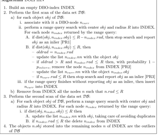
26 3 Outlier Detection in Data Algorithm DOLPHIN

1. Build an empty DBO-index INDEX 2. Perform the first scan of the data set DB:

a) for each object obj of DB:

i. associate with it a DBO-node ncurr

ii. perform a range query search with center obj and radius R into INDEX.

For each node nindex returned by the range query:

A. if dist(obj, nindex.obj) ≤ R − nindex.rad, then stop search and report

obj as an inlier [PR1]

B. if dist(obj, nindex.obj) ≤ R, then

– oldrad = nindex.rad

– update the list nindex.nn with the object obj

– if oldrad > R and nindex.rad ≤ R then, with probability 1 −

pinliers, remove the node nindex from INDEX [PR2]

– update the list ncurr.nn with the object nindex.obj

– if ncurr.rad ≤ R then stop search and report obj as an inlier [PR3]

iii. if the range query finishes without reporting obj as an inlier, then insert

ncurr into INDEX

b) Remove from INDEX all the nodes n such that n.rad ≤ R 3. Perform the second scan of the data set DB:

a) For each object obj of DB, perform a range query search with center obj and

radius R into INDEX. For each node nindexreturned by the range query:

i. if dist(obj, nindex.obj) ≤ R then

A. update the list nindex.nn with obj, taking care of avoiding duplicates

B. if nindex.rad ≤ R the delete nindex from INDEX

4. The objects n.obj stored into the remaining nodes n of INDEX are the outliers of DB

Fig. 3.1. The DOLPHIN distance-based outlier detection algorithm.

• DOLPHIN has been compared with state of the art distance-based outlier detection algorithms, specifically SNIF, ORCA, and RBRP, proving itself more efficient than these ones.

3.2 Algorithm

In this section the algorithm DOLPHIN is described. The algorithm uses a data structure called DBO-index (where DBO stands for Distance Based Outlier) defined next.

Let DB be a disk-resident dataset. First of all the definition of DBO-node is provided.

Definition 4. A DBO-node n is a data structure containing the following information:

(35)

3.2 Algorithm 27

• n.id: the record identifier of n.obj in DB;

• n.nn: a list consisting of at most k − 1 pairs (id, dst), where id is the identifier of an object of DB lying at distance dst, not greater than R, from n.obj;

• n.rad: the greatest distance dst stored in n.nn (n.rad is +∞ if less than k − 1 pairs are stored in n.nn).

A DBO-index is a data structure based on DBO-nodes, as defined in the following.

Definition 5. A DBO-index INDEX is a data structure storing DBO-nodes and providing a method range query search that, given an object obj and a real number R > 0, returns a (possibly strict) superset of the nodes in INDEX associated with objects whose distance from obj is not greater than R.1

Figure 3.1 shows the algorithm DOLPHIN. The algorithm performs only two sequential scans of the dataset.

During the first scan, the DBO-index INDEX is employed to maintain a summary of the portion of the dataset already examined. In particular, for each dataset object obj, the nodes already stored in INDEX are exploited in order to attempt to prove that obj is an inlier. The object obj will be inserted into INDEX only if, according to the schema described in the following, it will be impossible to determine that it is an inlier. Note that, by adopting this strategy, it is guaranteed that INDEX contains at least all the true outliers encountered while scanning the dataset.

After having picked the next object from the dataset, first of all, a range query search with center obj and radius R is performed into INDEX, and, for each DBO-node nindex encountered during the search, the distance dst

between obj and nindex.obj is computed.

Since nindex.rad is the radius of a hyper-sphere centered in nindex.obj and

containing at least k − 1 dataset objects other than nindex.obj, if dst ≤ R −

nindex.rad then within distance R from obj there are at least k objects and

obj is not an outlier. In this case, the range query is stopped and the next dataset object is considered.

Thus, this rule is used to early prune inliers. The more densely populated is the region the object lies in, the higher the probability of being recognized as an inlier through this rule. This can be intuitively explained by noticing that the radius of the hyper-spheres associated to the objects lying in its proximity is inversely proportional to the density of the region. This is the first rule used by the algorithm to recognize inliers. Since other rules will be used to reach the same goal, this one will be called Pruning Rule 1 (PR1 for short).

1 _{More precisely, assume that the method range query search is implemented}

through two functions, i.e. getFirst(obj,R), returning the first node of the re-sult set, and getNext(obj,R), returning the next node of the rere-sult set, so that candidate neighbors are computed one at a time.

(36)

28 3 Outlier Detection in Data

Otherwise, if dst ≤ R then the list nnindex.nn (nncurr.nn, resp.) of

the nearest neighbors of nindex.obj, (ncurr.obj resp.) is updated with n.obj

(nindex.obj resp.). In particular, updating a n.nn list with a neighbor obj

of n.obj, consists in inserting in n.nn the pair (obj, dst), where dst is the distance between obj and nn.obj. Furthermore, if after this insertion n.nn contains more than k − 1 object, than the pair (obj0_{, dst}0_{) in n.nn having the}

greatest value for dst0 _{must be deleted from n.nn.}

After having updated the nearest neighbors lists, if the radius nindex.rad

becomes less than R, then nindex.obj is recognized as an inlier. For clarity,

these objects are called in the following proved inliers. In this case there are two basic strategies to adopt.

According to the first one, the node nindexis removed from INDEX since it

is no longer a candidate outlier (recall that an object is inserted into INDEX only if it is not possible to determine that it is an inlier). This strategy has the advantage of releasing space as soon as it is not strictly needed, and maybe of making cheaper the cost of the range query search (when its cost is related to the size of INDEX), but it may degrade inlier detection capabilities since the PR1 becomes ineffective. Indeed, if this strategy is used, the field n.rad of each node n stored into INDEX is always +∞, otherwise the node n has to be cancelled from INDEX. According to the second strategy, the node nindex

is maintained into the index since it can help to detect subsequent dataset inliers through the PR1.

In between the above two strategies, there is a third intermediate one, that is to maintain only a percentage of the proved inliers. In particular, even though the latter strategy makes the PR1 effective, it must be said that it may introduce an high degree of redundancy. Being real data clustered, often objects share neighbors with many other dataset objects. Thus, it is better to maintain not all the proved inliers, but only a portion of them, say pinliers

percent. According to this third strategy, if nindex.rad is greater than R before

updating nindex.nn, but becomes less or equal to R after updating nindex.nn,

then, with probability pinliers, the node nindex is maintained into INDEX,

while with probability (1 − pinliers) it is removed from INDEX. This pruning

rule will be referred to, in the following, as PR2. The effect of the parameter pinliers, on the size of INDEX and on the ability in early recognizing inliers,

will be studied in the following.

As for the current dataset object obj, if ncurr.rad becomes less or equal to

R, then it is recognized as an inlier. In this case the range query is stopped, the object in not inserted into INDEX (this is the third pruning rule of inliers, PR3, for short, in the following), and the next dataset object is considered.

This completes the description of the first dataset scan. When the first dataset scan terminates, INDEX contains a superset of the dataset outliers. The goal of the second scan is to single out the true outliers among the objects stored in INDEX. Since the proved inliers stored in INDEX at the end of the first scan are no longer useful, they are removed from INDEX before starting the second dataset scan.

(37)

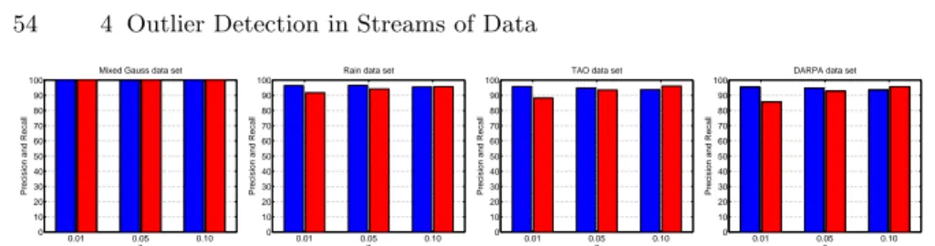
3.3 Analysis of the algorithm 29 0 100 200 300 400 500 0 0.2 0.4 0.6 0.8 1 Index size [m]

Probability of inserting the current object [p

m ] N=1000, x=95 k=20 k=5 (a) 0 200 400 600 800 1000 0 20 40 60 80 100 Circle, k=5, R=0.3

Number of dataset objects

Number of index nodes

pinliers=1.0 pinliers=0.1 pinliers=0.0 (b) 0 200 400 600 800 1000 0 50 100 150 200 250 300 Circle, k=20, R=0.3

pinliers=1.0 pinliers=0.1 pinliers=0.0 (c) 0 0.2 0.4 0.6 0.8 1 0 50 100 150 200 250 Circle, R=0.3 pinliers

Index size after first scan

k=20 k=5 (d) 0 100 200 300 400 500 0 0.2 0.4 0.6 0.8 1 Index size [m]

Probability of inserting the current object [p

m ] N=1000, x=499 k=100 k=25 (e) 0 200 400 600 800 1000 0 10 20 30 40 50 60 70 80 90 Clusters, k=25, R=0.400

pinliers=1.0 p inliers=0.1 pinliers=0.0 (f) 0 200 400 600 800 1000 0 50 100 150 200 250 300 Clusters, k=100, R=0.400

pinliers=1.0 pinliers=0.1 pinliers=0.0 (g) 0 0.2 0.4 0.6 0.8 1 0 50 100 150 200 Clusters, R=0.4 pinliers

Index size after first scan

k=100 k=25

(h) Fig. 3.2. Analysis of the algorithm.

During the second scan, for each dataset object obj, a range query search with center obj and radius R is performed into INDEX. This returns at least all the objects nindex.obj of INDEX such that obj lies in their neighborhood

of radius R. Thus, if dst, the distance between nindex.obj and obj, is less or

equal to R, the list of the nearest neighbors of nindex.obj can be updated using

obj. If nindex.rad becomes less or equal to R then nindex.obj is a proved inlier

and it is removed from INDEX.

At the end of the second dataset scan, INDEX contains all and only the outliers of DB. It can be concluded that, provided INDEX is a DBO-index, DOLPHIN returns all and only the outliers of DB after two sequential scans of DB.

3.3 Analysis of the algorithm

It immediately follows from the description of the algorithm, that the I/O cost of DOLPHIN corresponds to the cost of sequentially reading the input dataset file twice. This cost is really negligible even for very large datasets.

As for the CPU cost, it is related to the size of INDEX. Next it is investi-gated how the size of INDEX changes during the execution of the algorithm. 3.3.1 Spatial cost analysis

Interestingly, it can be provided evidence that, for meaningful combinations of the parameters k and R, even in the worst case setting where objects are not clustered and are never removed from INDEX, the size of any DBO-index INDEX at the end of DOLPHIN is only a fraction of the overall dataset.

Let N be the number of objects of the dataset DB. Say pmthe probability

(38)

30 3 Outlier Detection in Data

m, and assume that pinliers is one, so that no node inserted into INDEX is

removed during the first scan.

Let Ym be a random variable representing the number of objects to be

scanned to insert a novel object into INDEX when it already contains m objects. Assuming that the neighbors of a generic object are randomly picked from the dataset, i.e. that no relationship holds among the neighbors of the dataset objects, the problem is equivalent to a set of independent Bernoulli trials, and

pr(Ym= y) = pm(1 − pm)(y−1).

Hence, the expected number of objects to be scanned before inserting a novel object, when the index has size m is

E[Ym] = N X y=1 y · pr(Ym= y) = 1 pm . Consequently sm= m X i=1 E[Yi] = 1 p1 + . . . + 1 pm (3.1) is the expected number of dataset objects to be scanned in order to insert m nodes into INDEX. It can be concluded that the expected size of INDEX at the end of the first phase is SN = max{m | 1 ≤ m ≤ N and sm≤ N }.

Now we are interested in validating the above analysis by studying the growth of this function, and in empirically demonstrating that the value SN

is a worst case, since the size of INDEX is noticeable smaller for pinliers less

than one.

For simplicity, assume that each dataset object has approximately x neigh-bors. Also, assume that the outliers form a small fraction of the dataset, so that their presence can be ignored in the analysis. With this assumption, the probability that an inlier of DB, but out of INDEX, is inserted into INDEX (recall that it is supposed the neighbors of a generic object are randomly picked objects of the dataset) is

pm= Pk−2 j=0 ¡_n−x m−j ¢¡_x−1 j ¢ ¡_n−1 m ¢ (3.2)

which is the probability, conditioned to the fact that the current object is an inlier, that among the m objects of INDEX there are less than k − 1 neighbors of obj (p1= . . . = pk−2= 1, by definition).

Two synthetical datasets and a radius R such that x is almost constant for all the objects, were considered. The first dataset, named Circle, is composed by 1,000 points equally ranged over a circumference of diameter 1.0, plus a single outlier in the center of the circle. For R = 0.3 each point has x = 95 neighbors. The second dataset, named Clusters, is composed by two well-separated uniform clusters, having 499 points each, plus two outliers. For

(39)

3.3 Analysis of the algorithm 31

R = 0.4 each object has x = 499 neighbors, that are all the objects of the cluster it belongs to.

Figure 3.2(a) shows, for the Circle dataset, the probability pmof inserting

an inlier into INDEX, computed by using formula (3.2) with N = 1,000, x = 95, and k = 5 (solid line) and k = 20 (dashed line). Note that there exists a limit on the index size beyond which the probability of inserting becomes close to zero. Figures 3.2(b) and 3.2(c) show the expected size of INDEX versus the number of dataset objects processed (dashed-pointed line) computed by using formula (3.1). Figures 3.2(b) and 3.2(c) also show the actual size of INDEX for varying values of the parameter pinliers, that is pinliers= 0 (solid

line), pinliers= 0.1 (dashed line), and pinliers= 1 (dotted line).

Interestingly, if objects inserted in INDEX are never removed (pinliers =

1), then the observed final size of INDEX is below the value SN. This behavior

can be explained by noting that in real data common neighbors are biased. Moreover, if pinliersis decreased, then the final size of INDEX may be

notice-ably smaller than the value SN, even a little fraction of the overall dataset.

This behavior is confirmed by Figure 3.2(d), showing the size of INDEX at the end of the first phase of DOLPHIN as a function of pinliers for k = 5

(solid line) and k = 20 (dashed line).

Even though one may expect that by deleting all the proved inliers (pinliers = 0) the size of INDEX should be smaller (see Figure 3.2(b) for

an example of this behavior), it was observed that, in terms of maximum size of the index, the best value of pinliers is either a value close to 0.1 or exactly

zero, depending on the characteristics of the dataset.

Since, for meaningful combinations of the parameters k and R, very often the mean number of objects lying in spheres of radius R is high if compared with k, as we shall see, a value for pinliersslightly greater than zero is optimal

in practice in terms of execution time, and, sometimes, also in terms of index size. As an example, see Figure 3.2(c). For pinliers = 0, after INDEX has

accumulated enough objects to recognize inliers, the algorithm deletes the proved inliers from INDEX and forgets what has already seen. The size of the index becomes thus oscillating. The greater is the value of k, and the greater is the fluctuation of the size. On the contrary, for pinliers= 0.1, after

having accumulated in INDEX enough objects to recognize inliers, a large portion of proved inliers is removed but, since the algorithm has learned the dense regions of the feature space (this information is stored together with the proved inliers left into the index), the PR1 is applied efficiently and the size of the index stabilizes on a small fraction of the dataset. Using a greater value for pinliers has the effect of increasing the size of INDEX, but does not

augment the number of objects pruned by the PR1.

This behavior is much more evident on the dataset Clusters. Figures 3.2(e), 3.2(f), 3.2(g), and 3.2(h) report, on the Clusters dataset, the same kind of ex-periments described above (R = 0.4, x = 499). For pinliers= 0, the fluctuation

is now more pronounced as the objects are strongly clustered and the param-eter k is relatively large. Note that, for pinliers= 0.1 the final size of INDEX