dottorato di ricerca in fisica – xxiv ciclo
Gaetano Scandariato
THE INITIAL MASS FUNCTION OF
THE ORION NEBULA CLUSTER
FROM NEAR-INFRARED PHOTOMETRY
Ph.D. Thesis
Supervisor:
Prof. A.C. Lanzafame Tutors: Doct. I. Pagano Doct. M. Robberto Coordinator: Prof. F. Riggi anno accademico 2011/2012
“Fussiro tutti comu a tia. . . ” “Comu?”
“Forti. . . ”
Abstract 4
Introduction 6
1 Observations and data reduction. The catalog. 14
1.1 ISPI observations . . . 14 1.2 Data reduction . . . 15 1.2.1 Instrumental magnitudes . . . 18 1.2.2 Absolute calibration . . . 18 1.3 Completeness . . . 21 1.4 Results . . . 25
1.5 Analysis of the catalog . . . 25
1.5.1 Two-color diagrams . . . 25
1.5.2 Color-magnitude diagrams . . . 29
1.5.3 Luminosity Functions . . . 31
1.6 Summary . . . 35
2 The extinction map of the OMC-1 molecular cloud behind the Orion Nebula 37 2.1 Overview of previous studies . . . 38
2.2 The OMC-1 extinction map . . . 40
2.2.1 The extinction affecting each background star . . . 44
2.2.2 Computation of the extinction map . . . 45
2.2.3 Biases in the selection of background stars . . . 47
2.3 The Orion Nebula extinction map . . . 49
2.4 Discussion . . . 51
2.4.1 Structure of the OMC-1 beyond the Orion Nebula Cluster 51 2.4.2 Structure of the Orion Nebula . . . 53
2.5 Summary . . . 54
3 Empiric NIR colors for low-mass stars and BDs in the ONC 55 3.1 The data set . . . 57
3.2 Extraction of the reference stars . . . 58
3.2.1 Age spread . . . 58
3.2.2 Circumstellar Activity . . . 59
3.2.3 NIR excess from the inner disk . . . 60
3.3 Accuracy of the Allard et al. (2010) atmospheric model . . . 61
3.3.1 Sistematic uncertainties . . . 62
3.4 The empirical NIR isochrone of the ONC . . . 67
3.5 Comparison with other models and validation . . . 70
3.5.1 Magnitudes and colors vs. temperature . . . 70
3.5.2 Color-Magnitude Diagrams . . . 72
3.6 Summary . . . 72
4 The NIR excess of T Tauri stars in the ONC 76 4.1 The data set . . . 79
4.2 Observational evidences of NIR excess . . . 80
4.2.1 Stars without evidence for accretion . . . 82
4.2.2 Stars with accretion evidences . . . 83
4.2.3 Discussion . . . 84
4.3 The disk frequency . . . 87
4.3.1 Detection limit . . . 88
4.3.2 Disk frequency and trend with stellar mass . . . 89
4.3.3 Trend with stellar age . . . 90
4.3.4 Trend with projected cluster radius . . . 91
4.3.5 Discussion . . . 93
4.4 Summary . . . 94
5 The IMF of the ONC 96 5.1 The corrected Color-Magnitude Diagrams of the ONC . . . 96
5.1.1 Completeness correction . . . 97
5.1.2 Contaminant CMDs . . . 99
5.1.3 The intrinsic CMDs . . . 100
5.2 From photometry to the mass distribution . . . 100
5.2.4 The iterative algorithm . . . 106
5.3 The photometrically-determined IMF of the ONC . . . 108
5.3.1 Comparison with previous studies . . . 112
5.4 Summary . . . 115
Abstract
An important issue for the understanding of the star and planet formation process is the determination of the Initial Mass Function (IMF), in particular in the very low-mass and sub-stellar regimes, where recent investigations give controversial results.
The main goal of this thesis is the complete characterization of the IMF of the Orion Nebula Cluster (ONC) down to the Brown Dwarfs (BDs) regime, using ground-based Near-Infrared (NIR) photometric observations. The data taken in the framework of the Hubble Space Telescope (HST) Treasury Program on the ONC have been obtained with the wide-field imager Infrared Side Port Imager (ISPI) at the Blanco 4m telescope of CTIO, and cover an area of about 0.25 square degrees roughly centered on Θ1OriC. We observed the region in the
JHKS bands with exposure times of 330 s. As a result of our survey, we provide
2MASS-calibrated astrometry and photometry for ∼7000 sources in the ONC region.
Aiming at the photometric determination of the IMF of the ONC, we first clean the catalog for contaminants. We thus analyze the observed (H, H − KS)
Color-Magnitude Diagram (CMD), and we select a sample of bona-fide contam-inant background stars, deriving the interstellar reddenings by comparison with a synthetic galactic model. A statistical analysis is then performed to consis-tently account for local extinction, reddening and star-counts analysis in order to derive the background extinction map of the Orion Molecular Cloud 1 (OMC-1). The derived map has angular resolution <5′
and shows spatial structures of a few arcminutes and a general increase from the outskirts (AV ∼6) to the
direction of the Trapezium asterism (AV &30). Similarly, we select a sample of
bona-fide cluster members and we compare the observed colors to the expected colors for Pre-Main Sequence (PMS) stars, deriving the extinction map of the foreground Orion Nebula (ON) with angular resolution <7.′
5. The ON extinc-tion map is more irregular and optically thinner than the one of the OMC-1,
Orion molecular complex inside which star formation is still taking place. We then analyze a sample of ∼300 stars with previous measurements of luminosities, temperatures and simultaneous optical and NIR photometry. By analyzing their photospheric colors, we find that the synthetic JHKS
photom-etry provided by theoretical spectral templates for late spectral types (>K6) are accurate only to a level of ∼0.2 mag. We can thus provide an empirically-determined isochrone for low mass stars (spectral types later than K6) in the ONC, necessary to convert magnitudes into temperatures and masses.
Comparing the extinction-corrected magnitudes with our empirical isochro-ne, we derive the flux excess in the three JHKS bands, that we attribute to the
presence of a circumstellar disk. The observed fraction of disked stars (& 20% of the total sample) does not show any trend with stellar mass or stellar age. On the other hand, it increases with decreasing distance from the cluster center, consistently with the fact that the UV radiation field in the ON interacts with circumstellar disks forming the inflated structures known as “proplyds”.
Combining the previous results, we derive the contamination-completeness corrected (J,J-H) CMDs of the ONC, canceling out the contribution from the contaminant population. We also develop a statistical algorithm, which com-bines the CMD of the ONC with our reference isochrone and, taking into account the presence of extinction and NIR excess, derives the intrinsic Luminosity Function (LF) of the cluster. We finally combine the LF with our empirical NIR isochrone to derive a statistical estimate of the IMF at different distances from the cluster center. We find that the mass distribution of the cluster is peaked at ∼0.16 M⊙ and falls off crossing the hydrogen burning limit,
contin-uously decreasing in the BDs domain down to ∼0.03 M⊙. We also find that
the substellar-to-stellar objects ratio in the ONC decreases with increasing dis-tance from the cluster center, suggesting that BDs are preferentially formed in the deep gravitational potential well where the most massive stars of the Trapezium cluster are also found.
Introduction
A fundamental relation for understanding star formation and the evolution of stellar systems is the Initial Mass Function (IMF), that specifies the distribution in mass of a newly formed stellar population.
The shape of the IMF describes how long the galactic material will re-main locked up in stars of different masses, since the stellar mass determines both its lifetime and its contribution to enriching the interstellar medium with heavy elements, especially when it dies. During their life, intermediate-mass (1M⊙ <M<8M⊙) and massive stars (M>8M⊙) affect the interstellar medium
through radiation, outflows, winds and supernova explosions. When they die, they expel a large fraction of their mass, enriching the interstellar medium with elements heavier than H and He. On the other hand, lower-mass ob-jects, from Brown Dwarfs (BDs) (0.013M⊙ <M<0.075M⊙) to dim low-mass
stars (0.075M⊙ <M<1M⊙), retain most of their masses over cosmological time
scales. Consequently, the chemical evolution of galaxies is very sensitive to the IMF.
The importance of understanding the origin of the IMF and its apparent universality has therefore triggered much research on star formation, both the-oretical and observational. The history of the subject began in 1955, when E. Salpeter published the first estimate of the IMF for stars in the solar-neighborhood (d.100 pc) and found that it can be described by a power-law on a log N − log M histogram with slope α=1.35 in the range 0.4M⊙ <M<10M⊙
(Salpeter 1955). This result was then extended up to more massive stars (M≃20M⊙) (e.g. Massey 1998), while a significant flattening was found below
∼0.5M⊙ (Kroupa 2002).
Today the IMF has been estimated from low-mass BDs to very massive stars in a variety of systems. The regions that have been studied with direct star counts so far include the local field star population in our Galaxy and many star clusters and associations of all ages and metallicities in both our Galaxy and the
Magellanic Clouds. The sample ranges from present-day star-forming regions in small molecular clouds, to rich and dense massive star-clusters forming in giant clouds, up to ancient and metal-poor exotic stellar populations. This large body of direct evidence is consistent with the IMF being roughly the same for starbursts that have occurred under remarkably different circumstances and across the entire history of the Galaxy. Thus, the average IMF appears to be a universal function and can be approximately described by a power-law above 1M⊙, having a slope between 1 and 1.6, which is in agreement with the Salpeter
determination; below 1M⊙, the IMF shows a flattening down to 0.1M⊙or lower
(Kroupa 2002; Bastian et al. 2010).
Since at the moment there is no a priori reason to suppose that the IMF is a universal function, its apparent universality is a challenge for star formation theory; elementary considerations suggest in fact that the IMF should vary systematically with star-forming conditions, depending on the properties of the natal molecular cloud or of a nearby young stellar population (Elmegreen 1999). Given the still large uncertainties on the IMF determination, the question whether the differences in the observed IMFs under different star-forming con-ditions are real and significant is still an open issue. The IMF is particularly controversial in the very-low mass and substellar regimes. Recent studies have provided more information about Very Low Mass Stars (VLMSs) and BDs, confirming that the IMFs remains approximately constant or shows a moderate decline in the BDs regime. Nevertheless, there is no systematic indication of such a turnover, and certain regions have been found where the IMF appears to rise below the sub-stellar limit (Bastian et al. 2010, and references therein). If the shape of the IMF depends on the environment, it may offer vital insights into the physical processes that regulate the formation of stars and BDs and may also have strong implications for the choice of places in which to look for the most elusive BDs with mass comparable to those of giant planets.
The current differences in the sub-stellar IMFs may be ascribed to the fol-lowing reasons:
• an incomplete census for sub-stellar objects, due to the fact that the sur-veys for such objects concentrate sharply in selected sky areas, in partic-ular in the cores of star-forming regions;
• BDs may form only as unlucky members of small groups of stars, ejected by dynamical interactions before they can accrete to stellar masses
(Rei-8
purth & Clarke 2001). Hence, many sub-stellar objects might have es-caped detection in the pencil-beam surveys in star-forming regions; • alternatively, different processes (turbulent fragmentation, disk
fragmen-tation, core collapse, see e.g. Whitworth et al. 2007, for a review) can produce different initial conditions for star and planet formation, and hence might lead to different mass spectra in different star-forming re-gions. Also, the radiation and winds from OB stars or supernova shock waves that may trigger star formation in OB associations may also have an important effect on mass accretion during the formation process. While in a T association a protostar may accumulate a significant fraction of mass, the mass accretion of a low-mass protostar in a region exposed to the winds of OB stars or supernova shock waves can be terminated abruptly because of the photo-evaporation of the circumstellar matter (Kroupa 2001, 2002; Robberto et al. 2004). Therefore, many low-mass protostars may not complete their accretion and hence can result as sub-stellar objects. Spatially complete deep imaging surveys are then crucial in order to single out VLMSs and BDs with a minimum bias in the search strategy, and hence address problems like mass segregation in star-forming regions and the low end of the IMFs.
Wide-field imaging in the optical and especially in the infrared, as well as in the X-ray domain, are primary tools for the search of very low-mass Pre-Main Sequence (PMS) stars, young BDs and even giant free-floating planets. More-over, one has to take into account that young stellar objects can be interacting with a circumstellar accretion disk. The presence of the disk is revealed by the excess emission in the near-infrared (Meyer et al. 1997; Hillenbrand et al. 1998; Cieza et al. 2005; Fischer et al. 2011), mid infrared (Persi et al. 2000) and far-infrared (Prusti et al. 1992), while the magnetically funneled accretion columns produce broadened emission lines (i.e. strong Hα emission, etc.
Hart-mann 2009). X-ray emission from low-mass PMS stars, on the other hand, is likely to be originated, as in the Sun, from their surface activity involving a dynamo generated magnetic field (Feigelson & Montmerle 1999) and may be therefore less sensitive to the presence of accretion.
In recent years it has been shown that young BDs are also X-ray emitters and may exhibit strong Hα emission (Jayawardhana 2010). The ubiquity of
sce-nario for VLMSs and BDs. Therefore, all the phenomenological characteristics regarding PMS activity can be extrapolated, at a smaller scale, to the BDs regime.
The importance of the Orion Nebula Cluster
The IMF inferred for the local field stars is subject to significant uncertainty because it depends on the assumed evolutionary history of the local Galactic disk and on the assumed stellar lifetimes. In general, determining the IMF of a stellar population with mixed ages requires strong assumptions. Stellar masses cannot be measured directly in most cases, so the mass has to be deduced indirectly by measuring the star luminosity and the spectral type; mass measurements are then affected by the errors on the star distance and the accuracy of theoretical stellar models, which are rather uncertain particularly in the low-mass and substellar regimes (Baraffe et al. 2002).
In contrast, the IMF of homogeneous star clusters or associations can be derived with fewer assumptions and should be more reliable, since all of the stars in each cluster have roughly the same distance and age and, at least in the youngest clusters, all of the stars are still present (with a few possible exceptions for runaway stars) and can be directly counted as a function of mass without the need for evolutionary corrections. The best time to determine the IMF is then early in the life of a cluster or association, before high mass stars burn out and dynamical friction ejects the lower mass systems.
Another important issue is that the luminosity of PMS VLMSs and BDs is a decreasing function of age. Their bolometric luminosity during the gravo-thermal contraction phase evolves with time approximately as t−1/2(Black 1980;
Burrows et al. 1995). Therefore, it may also be easier to detect VLMSs and BDs in star-forming regions, when they are very young. Thus, at ages of a few Myr, one can more readily reach masses below the hydrogen-burning limit. For example, at this age, a 0.075M⊙ object (i.e. the high mass limit for a BD)
is as luminous as a 0.35 M⊙ mid-M spectral type star on the main sequence,
according to the current evolutionary models.
The Orion Nebula (ON) (M42, NGC 1976) (Fig. 1.7) hosts the richest cluster of young (τ ≃1-2 Myr) PMS stars within 1 kpc of the Sun: the Orion Nebula Cluster (ONC) (see Muench et al. 2008; O’Dell et al. 2008, for recent reviews). The ON can be characterized as a bright blister of ionized gas on the surface
10
of the Orion Molecular Cloud 1 (OMC-1). The rapid expansion of the HII region, powered by a small number of massive OB stars mostly clustered in the Trapezium multiplet (θ1 Ori) (O’Dell et al. 2008, 2009), has exposed to our
view the ONC, an extremely rich aggregate of PMS stars ranging from 45 M⊙ to
less than 0.02 M⊙. A foreground veil of neutral gas, marginally optically-thick,
passes through the nearest members of the ONC. The NW part of the nebula, designated M43 (NGC1982), is illuminated by NU Ori (Sp.Type BIV) with its own associated cluster. Two additional sites of embedded star formation are projected on the core region: 1) the cluster associated with the BN-KL infrared sources, ∼1′
NW of the center; 2) the Orion-S sources, with numerous HH sources, ∼1′
SW of the center. Both clusters are younger than the ONC, but the ONC is by far the richest, having bona-fide members located up to the edges of the nebula.
Because the ONC is one of the nearest massive star-forming regions to the Sun and the most populous young cluster within 1 kpc, it has been observed at virtually all wavelengths over the past several decades. However, only re-cently the increased sensitivities of the Near-Infrared (NIR) detectors on larger telescopes allowed us to begin to understand and characterize the extent of the ONC’s young stellar and BD population, which, at ∼1–2 Myr, is just begin-ning to emerge from its giant molecular cloud OMC-1. The whole program was designed to study the ON in great detail. We take advantage of the fact that it is close (d∼400 pc), lies well below the Galactic Plane (b=-19), and in an anti-center quadrant (l=209) with minimal foreground confusion. It lies on the front edge of the OMC-1 Giant Molecular Cloud, whose total extinction (up to AV=50-100 on the main ridge) eliminates background confusion. The
moderate foreground extinction (AV .0.5) allows detailed studies at visible and
NIR wavelengths of individual stars. The richness of the stellar cluster (n∼3500 stars) and its density (∼2·104 stars pc−3 at the core, Hillenbrand & Carpenter
2000) make the ONC a unique target for wide-field imaging. In addition, a number of deep NIR surveys (Hillenbrand et al. 1998; Lucas & Roche 2000; Luhman et al. 2000; Muench et al. 2002) indicate that there are >200 PMS BDs, and perhaps tens of objects below the D-burning limit of 0.013 M⊙, in the
ONC core. Substellar objects are a thousand times brighter at an age of a few Myr than at an age of a few Gyr: this property, combined with the strategic projected position of the cluster in the sky, makes the ONC the ideal laboratory to study the low-mass end of the cluster IMF.
In the last decade, several studies have explored the ONC at substellar masses. Hillenbrand & Carpenter (2000) present the results of an H and KS
imaging survey of the inner 5′
×5′
region of the ONC. Observed magnitudes, colors, and star counts were used to constrain the shape of the ONC mass function across the hydrogen-burning limit down to 0.03 M⊙. They find evidence
in the log N − log M mass function for a turnover above the hydrogen-burning limit, then a plateau into the substellar regime. A similar study by Muench et al. (2002) uses J, H and KS imaging of the ONC to derive an IMF that
rises to a broad primary peak at the lowest stellar masses between 0.3 M⊙ and
the hydrogen-burning limit before turning over and declining into the substellar regime. However, instead of a plateau through the lowest masses, they find evidence for a secondary peak between 0.03 M⊙ and 0.02 M⊙. Luhman et al.
(2000) use H and KS infrared imaging and limited ground-based spectroscopy
to constrain the mass function and again find a peak just above the substellar regime but then a steady decline through the lowest mass objects.
Generally speaking, photometry alone is not sufficient for deriving stellar masses but, on the other hand, it is adequate in a statistical sense for estimating mass distributions given the right assumptions. This is a great advantage with respect to spectroscopy, as it allows to collect data for a large number of stars in a limited observational time. On the other hand, the position of a PMS star in the Color-Magnitude Diagram (CMD) is dependent on mass, age, extinction, and the possible presence of circumstellar activity (either accretion processes or the presence of a circumstellar disk). These characteristics affect the conversion of a star’s magnitudes and colors into its stellar mass.
Specifically for the ONC, photometric observations are hampered by the brightness and non-uniformity of the nebular background. To overcome ob-servational difficulties and theoretical uncertainties, the unique combination of sensitivity and spatial resolution offered by the Hubble Space Telescope (HST) has been exploited to obtain accurate photometry of the cluster, especially at substellar masses (HST Treasury program GO-10246). The HST survey has been complemented by ground-based observations, imaging the ON from the U-band to the KS-band at La Silla and Cerro Tololo (CTIO) observatories. The
ground-based observations, carried out in parallel on the same nights (but at a different epoch than the HST observations), complement the deep HST data which saturate at relatively low brightness levels. Their simultaneity makes the derived stellar colors largely immune to the uncertainties associated with
12
photometry collected at different epochs.
Outline
In the following chapters we aim at the complete characterization of the ONC down to the BDs regime, using the ground-based NIR JHKS photometric
observations presented in Chapter 1. In particular, the main objective of the program is to derive the photometrically-determined IMF of the cluster. As discussed in Lada & Lada (2003), to achieve this goal one needs the intrin-sic Luminosity Function (LF) of the cluster and the most appropriate Mass-Luminosity Relation (MLR). In order to derive the intrinsic LF, the first step is to correct the observed LF for galactic and extragalactic contamination. To this purpose, in Chapter 2 we extract a sample of bona-fide background stars from the catalog and analyze their projected spatial density and color excess to derive the extinction map of the OMC-1. We then combine this map with the galactic population model to derive a statistical estimate of the contaminant LF as seen through the bulk of the OMC-1, to be subtracted from the observed LF.
Another correction needed in order to derive the intrinsic LF is the removal of the NIR excess due to circumstellar disks. To achieve this goal, we first cross-match our NIR catalog with previous spectro-photometric optical observations, selecting a sample of ONC members with no evidence of flux excess due to accretion and/or circumstellar disks. Combining the observed colors of these stars with previous determinations of their Teff, we derive the empirical NIR
isochrone of the ONC (Chapter 3).
With this empirical isochrone at hand, which is meant to closely reproduce the intrinsic colors of the ONC members, in Chapter 4 we analyze the amount NIR excess entering our observed photometry. In particular, we use the sub-sample of ONC members with spectral type to compare the expected colors of stars with the corresponding extinction-corrected colors. We thus derive the excess in the three JHKS bands and we find that correlations between them are
consistent with a circumstellar disk thermally radiating in the NIR.
Combining the previous results, in Chapter 5 we present a numerical method which simultaneously takes into account the effects of interstellar extinction and NIR excess, using the full set of observed JHKSmagnitudes. Our algorithm also
incidence of galactic contamination consistently with the extinction provided by the OMC-1. This allows us to statistically derive the intrinsic NIR LF of the ONC. We then combine the LF with the empirical isochrone, and we derive the complete IMF of the ONC down to the BDs domain.
Chapter 1
Observations and data
reduction. The catalog.
1.1
ISPI observations
The Infrared Side Port Imager (ISPI) is the facility infrared camera at the CTIO Blanco 4 m telescope. ISPI uses a 2k×2k HgCdTe HAWAII-2 array, with reimaging optics providing a scale of 0.3′′
/pixel corresponding to a 10.′
25×10.′
25 field of view. Our target area, about 30′
×40′
, covers the field imaged with the HST.
The observations were performed on the nights of 1 and 2 January 2005 (indicated hereafter as Night A and Night B respectively) in the J, H and KS
filters using the Double Correlated Sampling readout mode. The main filter parameters are listed in Table 1.1. The seeing was ≃0.′′
7 in most of the KS-band
images and occasionally worse on night B.
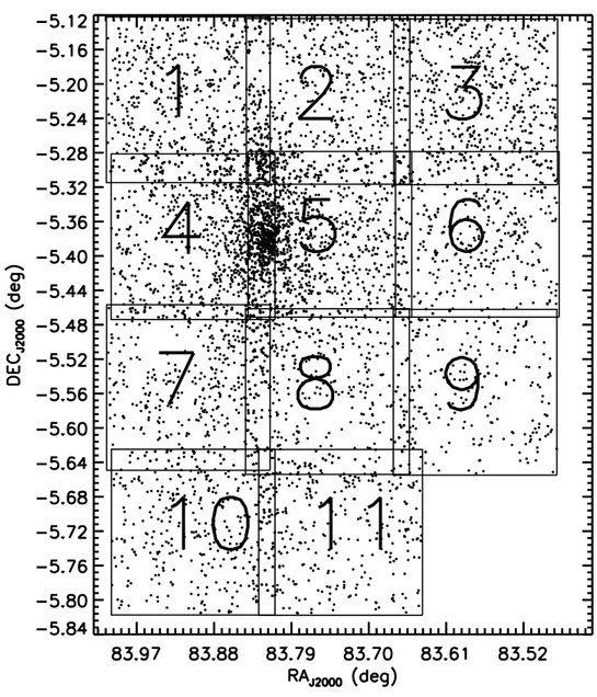
The survey area was divided into eleven fields (Fig. 1.1). The central po-sition of each field, together with the airmass of the observations, is listed in Table 1.2. Each field was observed with an ABBA pattern. After pointing the telescope to the center of a field (A position) a 5 point dithering pattern was executed offsetting the telescope approximately by ±30′′
along the field diago-nals. This first group of 5 dithered exposures was followed by a second group
Table 1.1: ISPI Broad Band Filters.
Filter Central wavelength (µm) ∆λ (80%) (µm)
J 1.250 1.176 - 1.322
H 1.635 1.500 - 1.770
KS 2.150 1.992 - 2.300
Table 1.2: Log of the ISPI observations.
Field Night RA (2000.0) DEC (2000.0) Airmass 1 A 05:35:38.37 -5:12:50.7 1.144 - 1.291 2 A 05:34:59.63 -5:12:57.6 1.123 - 1.139 3 A 05:34:18.52 -5:12:59.6 1.123 - 1.139 4 A 05:35:37.05 -5:22:38.6 1.309 - 1.158 5 A 05:34:59.08 -5:22:28.3 1.319 - 1.938 6 A 05:34:17.98 -5:22:28.3 1.319 - 1.938 7 B 05:35:38.16 -5:33:03.8 1.218 - 1.410 8 B 05:34:59.82 -5:33:18.6 1.104 - 1.211 9 B 05:34:18.50 -5:33:21.4 1.104 - 1.211 10 B 05:35:37.48 -5:43:06.9 1.110 - 1.215 11 B 05:34:56.28 -5:43:09.2 1.110 - 1.215
of sky frames (B position) taken on a nearby field free, or nearly free, of diffuse nebular emission to extend the field coverage and monitor the flat-field response close in time to our observations. The sky-source sequence was then repeated back, completing the ABBA cycle. This provides a total of 10 frames of 30 s exposure for the common part of each field, totaling 300 s integration. Due to the high background, we split the KS-band 30 s exposures in two consecutive
15 s exposures, maintaining the background well within the linear regime. Each dithering sequence was repeated with a 3 s integration time. These short frames were coadded into another image of 30 s total integration time, which we used to extract the photometry of sources saturated in the longer exposures. Due to an error in our observing procedure, the J-band observations of field 3 were obtained only with 3 s exposures.
For absolute calibration we observed at various airmass the faint IR standard stars 9108, 9118 and 9133 of Persson et al. (1998). Unfortunately, on both nights the atmospheric transmission at IR wavelengths turned out to be unstable due to variations in the water vapor opacity, and we eventually derived the zero point calibration of our images through comparison with the extensive set of 2MASS data across our wide field area, as described in Sect. 1.2.2.
1.2
Data reduction
The first step in the data reduction was the correction for the intrinsic non-linearity of the detector, which we performed by applying the correction curve
1.2 Data reduction 16
Figure 1.1: Position of the eleven ISPI fields, superimposed to the positions of the sources detected in our survey.
kindly provided by N. Van der Bliek1. We flat-fielded each image using dome
flats and correct for residual color terms at low-spatial frequency using delta-flats derived from median averaged sky images. The dome delta-flats were also used to flag bad pixels. The sky frames, properly filtered to remove spurious sources arising from the latent images of bright stars on the infrared detectors, were combined and subtracted from the science images.
Since ISPI exhibits significant field distortion, each science image had to be geometrically corrected before being combined in a dithering group. This required a first pass of aperture photometry with DAOPHOT, in order to extract a source catalog with well measured centroids and photometry (to disentangle the case of multiple candidates in the search radius). These sources were then cross-identified with the 2MASS catalog for astrometric reference, building an image distortion map relating their position on the original images to the actual position provided by 2MASS.
Due to the non-uniform distribution of sources, clustered at the center of the nebula, the accuracy of the distortion correction map varies across each field. Therefore, we combined the distortion maps relative to all images taken on the same night to derive, for each filter, a master distortion map. Each individual image was then warped using a 4th-order polynomial fit with coefficients derived from the corresponding distortion map.
Images belonging to the same dithered groups were then combined per in-teger pixels into single 2500×2500 images. The DAOPHOT source extraction was then repeated on these geometrically corrected images to produce a new source catalog from which we derived the final astrometric solution of each im-age by minimizing the residual shift and rotation with respect to the 2MASS positions. The average scatter between our coordinates and the corresponding 2MASS coordinates turns out to be about 0.15′′
, i.e. half of a ISPI pixel. The same procedure has been adopted on the 3 s images.
In conclusion, for each field the final data consist of one combined image in each of the 3 filters (J, H, KS) and exposure times (300 s and 30 s), with the
exception of fields 4, 5, and 6, which have double this number of images, and field 3, which was not observed with deep J images.
1now also available on the ISPI web page: http://www.ctio.noao.edu/instruments/
1.2 Data reduction 18
1.2.1
Instrumental magnitudes
The extraction of source photometry was performed on the final combined im-ages, for both short and long exposure times. The Daophot FIND IDL proce-dure was used to extract an initial list of candidate sources, with rather loose detection thresholds and criteria to include the largest possible number of candi-dates. This initial list, counting more than 60,000 candidates, has been visually inspected on the original images to clean up artifacts and to preliminarily clas-sify real sources as either point-like or extended. The list was then reduced to 7563 sources, divided between 6630 point-like and 933 diffuse.
For all sources we first derived an aperture magnitude by integrating the flux over a 5 pixel (1.5′′
) radius circular aperture, taking sky annuli typically between 10 and 15 pixels (3.0-4.5′′
); for 1416 bright sources, saturated in the 30 s images, we used the photometry extracted from the 3 s images.
We then performed Point Spread Function (PSF) photometry on all point-like sources. Due to the spatial variability of the PSF across the field of view of ISPI, present even after geometric correction, we divided each image in 9 parts (3×3 squares) allowing for some overlap between adjacent sub-images. The samples of stars in each sub-image, still relatively rich, had a more homo-geneous PSF allowing us to reliably derive PSF magnitudes. We subtracted the PSFs and looked at the residual images searching for faint companion stars previously undetected. We found in this way 325 “hidden companions”. Fi-nally, we performed a second pass of PSF photometry, first by removing from the list of stars used to derive the PSF those having a faint companion, and then deriving also the photometry of the newly detected faint companions.
1.2.2
Absolute calibration
As mentioned in Sect. 1.1, the IR photometric quality of our nights turned out to be unsatisfactory due to hygrometric variability. We therefore calibrated our ISPI instrumental magnitudes directly to the 2MASS photometric system. The 2MASS catalog provides absolute photometry in the J (1.25µm), H (1.65µm), and KS (2.17µm) bands to a limiting magnitude of 15.8, 15.1, and 14.3,
respec-tively, with Signal-to-Noise Ratio (SNR) greater than 10.
To estimate the color terms and zero points of each image, we first scaled the instrumental PSF magnitudes of point sources measured in the short 30 s images to the long 300 s images, chosen as the reference time because of their source
richness. To minimize systematic effects due do atmospheric variations, we did not simply add the nominal ∆mag=2.5 factor but compared the instrumental magnitudes of well measured stars to derive for each field and filter a mean magnitude offset ∆mag between the short and long images. By homogenizing in this way the zero points of the short and long images, we add a small uncertainty to the photometric errors of the bright stars measured in the short exposures.
For each bandpass λ we then evaluated the relations
mag2MASS(λ) − magISPI(λ) = ZPλ+ ǫλ1,λ2 ·cISPI(λ1, λ2),
where mag2MASS is the magnitudes in the 2MASS photometric system, magISPI
is the ISPI instrumental magnitude, the intercept ZPλ is the zero point in a
given bandpass, the slope ǫλ1,λ2 is a color coefficient between the wavelengths
λ1 and λ2 and cISPI is the corresponding observed ISPI color. We found the
strongest statistical correlation in the combination:
H2MASS−HISPI= ZPH + ǫJK·(J − K)ISPI.
For each field, we derived the linear fit parameters ZPH and ǫJK using
an iterative procedure to rejects spurious outliers and all sources with errors greater than 0.1m in the 2MASS catalog and 0.05m in our input catalog. As
shown in Table 1.3, the color coefficient ǫJK varies slightly from field to field
during each night, whereas the zeropoint ZPλ shows an increase towards the
middle of the night (observation were scheduled with fields 4 and 10 transiting at the meridian, in the two nights).
For the J and KS bands, we derived the zero-points and the color terms from
a linear fit to the color relations
(J − H)2MASS= ZPJH+ ǫJH ·(J − H)ISPI,
(H − KS)2MASS= ZPHK+ ǫHK ·(H − KS)ISPI.
This allowed us to derive magnitudes calibrated in the 2MASS system for all sources with ISPI JHK instrumental photometry. In Fig. 1.2 we show a com-parison between the magnitudes reported in the 2MASS catalog and our cali-brated magnitudes. The plots show the lack of systematic differences, besides the random errors that we attribute to photometric errors or stellar variability. For sources lacking one or two magnitudes (typically either J or both J and H), we assumed a linear relation of this type
1.2 Data reduction 20
Table 1.3: Best estimate for calibration coefficients Field ZH σZH ǫJK σǫJ K 1 1.09 0.01 -0.010 0.008 2 1.07 0.01 0.001 0.007 3a 1.08 0.04 0.00 0.02 4 1.13 0.01 -0.022 0.006 5 1.11 0.01 -0.023 0.007 6 1.03 0.02 -0.05 0.02 7 0.93 0.02 0.00 0.01 8 0.93 0.01 -0.023 0.008 9 0.95 0.01 -0.02 0.01 10 1.09 0.02 -0.06 0.01 11 1.07 0.02 -0.02 0.01
Notes. (a) Parameters for field 3 are computed using non-normalized J-band
mag-nitudes.
Figure 1.2: Comparison between 2MASS magnitudes and ISPI calibrated mag-nitudes.
Figure 1.3: PSF photometric error as a function of magnitude for our point-like sources. The solid red line indicates the locus of the average relation for the 2MASS sources falling in the ISPI field.
deriving α and β, for each bandpass and field, from the sample of calibrated sources. The parameter α provides a magnitude-dependent correction to the zero point β, which is appropriate since fainter sources have, on average, redder colors. Using these coefficients we calibrated the magnitudes, with the relative uncertainties, of all remaining sources.
Figure 1.3 shows the photometric errors plotted as a function of magni-tude for all point-like sources. The multiple threads in the distribution of the photometric errors are due either to the superposition of deep and short expo-sures (bright stars, measured in short 3 s expoexpo-sures, turn out to have relatively larger errors) or to the sources measured, with higher photometric errors, in the crowded central part of the cluster. For comparison we also plot the average mag vs. ∆mag relation for the 2MASS sources falling in our field.
1.3
Completeness
To determine the completeness of our photometric catalog, we used an artificial star experiment. For each field and filter, we averaged the 9 PSFs created for photometric extraction (Sect. 1.2.1) into a common reference PSF valid for the full image. We scaled the reference PSF in steps of 0.1 mag covering the entire magnitude range measured across each field and injected each scaled PSF at a random position in the image, with the only caveat of leaving enough distance from the border to allow for a meaningful measure. We assumed as a detection criterion a photometric error less than 0.3 mag and less than 0.5 mag difference between the injected and recovered magnitude, making also sure that the stars
1.3 Completeness 22
recovered by the code were the artificial ones and not previously known real stars. The completeness was calculated as the fraction of successful detection after 10000 iterations of the process, for each magnitude bin.
It turns out that the completeness (and the sensitivity) of our survey is signif-icantly affected by the nebular brightness. We have therefore defined three con-centric regions (Fig. 1.4) at increasing distance from Θ1OriC (RA (2000.0)=05h
35m 16.46s, DEC (2000.0)=-05◦
23′
23.′′
18). The limiting radii, respectively 6.′
7, 14.′
3 and 27.′
2 (corresponding to projected distances of 0.81, 1.72 and 3.27 pc at a distance of 414 pc (Menten et al. 2007)) have been set in such a way that the three regions contain the same number of point-like sources. In order to avoid significant contamination from the M43 cluster, we neglect in our anal-ysis a circle with a 5′
radius centered on NU Ori (RA(2000.0)=05h35m31.37s,
DEC(2000.0)=-05◦
16′
02.′′
6) (see Fig. 1.4).
The results of our simulations are shown in Fig. 1.6. For each filter, the com-pleteness estimated in the outer region is slightly, but systematically, larger than that in the intermediate region, which in turn is much larger than in the bright inner region, the most heavily affected by crowding and diffuse emission, where our sensitivity begins to drop at HKS ∼14 mag. A comparison with Hillenbrand
& Carpenter (2000) and Muench et al. (2002), who surveyed the inner part of the cluster (5′
×5′
and 6′
×6′
fields, respectively) deriving HK photometry down to our photometric limit (KS∼18 mag), shows that we detect as point sources
more than 90% of their sources (648/706 in the H-band and 657/698 in the KS-band for Hillenbrand & Carpenter (2000) and 601/662(H) and 665/714(KS)
for Muench et al. (2002)). Figure 1.5, where we overplot the LFs obtained by Hillenbrand & Carpenter (2000) and Muench et al. (2002) (dashed lines) to our observed LFs (gray area) constructed for their same regions, confirms that the missing sources are generally fainter than HKS≃14 mag (the missing bright
sources, detected but not measured by ISPI due to saturation, are not relevant here). If we apply to our H and KS LFs the appropriate completeness
correc-tions, estimated by repeating the artificial star experiment on the same fields of Hillenbrand & Carpenter (2000) and Muench et al. (2002), our LFs become con-sistent with theirs, with the exception of the secondary peak at KS≃15.5 mag
discussed by Muench et al. (2002). In Sect. 1.5.3 we will apply the completeness corrections to the measured counts, when we will compare the LFs at various distances from the cluster center.
Figure 1.4: Projected regions identified in our surveyed area. The solid cir-cles define the three radial areas containing an equal number of point-like sources, with radii of 6.7′
, 14.3′
and 27.2′
respectively. The dashed circle in-dicates the exclusion field centered around NU Ori. The positions of Θ1OriC, Θ2 Ori and NU Ori are also indicated, together with our original field positions.
The axes show the angular offsets from Θ1OriC (RA (2000.0)=05h 35m 16.46s,
DEC (2000.0)=-05◦
23′
23.′′
1.3 Completeness 24
Figure 1.5: Dashed lines: H and KS luminosity functions for the Hillenbrand
& Carpenter (2000) (upper panels) and Muench et al. (2002) (bottom panels) catalogs; gray area: luminosity functions for the same filter and fields from the ISPI observations (point sources only); solid line: ISPI luminosity func-tions corrected for completeness. The error bars have been obtained by adding quadratically the statistical (poissonian) uncertainty on the measured counts to the completeness correction error derived from the Monte Carlo simulations.
Figure 1.6: Completeness levels for the J (left), H (center) and KS (right) bands
derived from the artificial star experiment. Each plot shows the results for the 3 radial regions.
1.4
Results
Our final photometric catalog contains 7759 sources. Having visually inspected all sources, we find that 6630 can be classified as point-like sources and 933 as diffuse objects. The other 174 sources, typically brighter than KS≃10, turned
out to be saturated even in our short 3 s images. We included them in our catalog, adopting the photometry and coordinates reported by 2MASS. We also found that the 2MASS photometric catalog misses 22 sources in the Trapezium region clearly visible in the 2MASS images and saturated even in our short exposures. We have added their JHKS photometry using the Muench et al.
(2002) photometry.
In Table 1.4 we summarize the number of sources measured in different combination of filters, exposure times, and morphological types. The source catalog is available at Centre de Donn´ees astronomiques de Strasbourg (CDS). Figure 1.7 shows a JHKS color composite of our imaged field. The image,
produced by the graphic staff of the Space Telescope Science Institute, has been artificially enhanced to reduce the original dynamic range and more clearly reveal the inner part of the cluster.
1.5
Analysis of the catalog
1.5.1
Two-color diagrams
In Fig. 1.8a we show the NIR J-H versus H-KS Two-Color Diagram (2CD) for
1.5 Analysis of the catalog 26
Figure 1.7: NIR color composite mosaic of the ON from our ISPI images. The image has been digitally enhanced to improve the visibility of the stellar sources in the central region. The RGB colors code the KS, H and J bands, respectively.
Table 1.4: Source Summary.
Source Number of stars
ISPI detected in J-, H- and KS-bands 4851
ISPI detected in J- and H-bands, not in KS-band 92
ISPI detected in H- and KS-bands, not in J-band 1096
ISPI detected in J- and KS-bands, not in H-band 85
ISPI detected only in J-band 175
ISPI detected only in H-band 80
ISPI detected only in KS-band 251
ISPI diffuse 933
ISPI Total 7563
Extracted from the 2MASS catalog 174
Extracted from the Muench et al. (2002) catalog 22
Grand Total 7759
ISPI detected in 30 s images 6147
ISPI detected in 3 s images 1416
ISPI first run detection 6305
ISPI hidden companions 325
ISPI diffuse 933
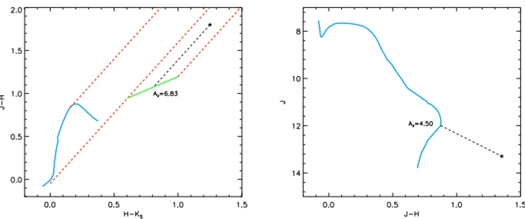
the main-sequence stars and giant branch, together with the locus of Classical T Tauri Stars (CTTSs) surrounded by circumstellar disks (Meyer et al. 1997), given by the relation (J-H)-0.630(H-KS)-0.497=0 in the 2MASS photometric
system. We also plot the interstellar reddening vector of Cardelli et al. (1989), given by the relation E(J-H)/E(H-KS)=1.83 in the 2MASS photometric system.
Accounting for extinction, the locus of the CTTSs lies between the two parallel dotted lines defined by the equations (J-H)-1.83(H-KS)+0.098=0 and
(J-H)-1.83(H-KS)+0.50=0.
For 45.2% (1853/4103) of the sources, the NIR colors are consistent with those of stellar dwarfs (luminosity class V), giants (luminosity class III) or CTTSs reddened by various amounts of foreground extinction. For 11.4% (466/4103) of the sources the NIR excess is compatible only with the red-dened CTTSs, whereas only 0.8% (35/4103) of the sources show NIR excess significantly greater than those of CTTSs, indicative of strong KS-band excess.
To assess how the observed reddening and color excess vary with the dis-tance from the center of the cluster, we consider the so-called Hess diagrams (i.e. the density distribution diagrams) for the three radial regions. The inner field (Fig. 1.8b) shows a peak well detached from the main sequence, with iso-density contours elongated in a direction parallel to the CTTSs locus, together
1.5 Analysis of the catalog 28
Figure 1.8: a) top-left panel : NIR 2CD diagrams for selected point-like sources in our catalog detected in all 3 bands (see text for the selection criteria). Also shown are the main-sequence (magenta solid line), the giant-branch (red solid line) sequence and the CTTSs locus by Meyer et al. (1997) (green solid line). The dotted lines are parallel to the standard reddening vector. b) (top-right panel) - Hess diagrams of the color-color diagram relative to the inner region. c) bottom-left panel : Similar to panel b), for the median region. d) bottom-right panel : Similar to panel b) for the outer region.
with a long tail of stars with high reddening. The Hess diagram for the inter-mediate region (Fig. 1.8c) shows a main peak much closer to the locus of dwarf stars, together with a secondary maximum at higher extinction. The interme-diate contour levels (e.g. the green area) are now elongated along the range of reddened main sequence stars.
Finally, the Hess diagram for the outer region (Fig. 1.8d) shows again a strong peak compatible with dwarf stars affected by a small amount of extinc-tion, whereas the low contour levels appear less pronounced than in the two other regions and well within the limits of reddened main sequence or giant stars.
Overall, the three 2CDs can be interpreted as follows: 1) the inner Trapez-ium region is mostly populated by young stars with NIR excesses typical of CTTSs. They have generally relatively modest amounts of extinction, which is compatible with the fact that the ionizing radiation from the Trapezium stars has cleared the molecular cloud and exposed them to our view; 2) the inter-mediate region contains a relatively larger number of heavily reddened sources. They are seen through denser parts of the OMC-1, not yet reached by the ex-pansion of the ionized cavity; 3) the outer regions mostly contain background objects seen trough the low opacity layers at the edges of the main OMC-1 ridge, which crosses the ONC approximately in north-south direction (Goldsmith et al. 1997).
1.5.2
Color-magnitude diagrams
In Fig. 1.9 we present the (H, J-H) and (KS, H-KS) CMD still for the same
sample. Together with our data, we plot the 1 Myr isochrone of Chabrier et al. (2000), which covers the range 0.001 M⊙ < M < 0.1 M⊙ and is tailored
to model substellar and planetary mass objects in the limit of high opacity photospheres. We also plot the 1 Myr isochrone of Siess et al. (2000) ranging from 0.1 M⊙ to 7 M⊙, well-suited for stellar sources. Both isochrones have
been converted to the 2MASS photometric system using the transformations of Carpenter (2001). The offset between the two isochrones can be regarded as a graphic representation of the uncertainties in theoretical models. An AV = 10
reddening vector is also indicated, as well as the reddening lines starting from the isochrones in correspondence of a 1 M⊙ object (J=10.50, H=9.88 and KS=9.76
1.5 Analysis of the catalog 30
Figure 1.9: NIR CMDs for selected point sources in our catalog detected in all 3 bands, with 1 Myr isochrones, assuming a distance d = 414 pc (DM = 8.01). To derive these isochrones, we used Chabrier et al. (2000) combined to the Siess et al. (2000) model, as discussed in Sect. 1.5.2. The AV=10 mag reddening vector
is also shown. The diamond symbols represent the positions of a M = 0.012 M⊙
(deuterium burning limit) object, a M = 0.075 M⊙ (hydrogen burning limit)
object and a M = 1 M⊙ star from bottom to top respectively.
hydrogen-burning limit mass (J=14.29, H=13.86 and KS=13.56 at 414 pc in
the 1 Myr Chabrier00 isochrone) and a M = 0.012 M⊙ substellar object at
the deuterium-burning limit mass (J=17.33, H=16.90 and KS=16.48 at 414 pc
in the 1 Myr CBAH00 isochrone). For this distance and isochrone, our survey is therefore sensitive to stellar sources down to AV ≃60, BDs down to AV ≃ 40,
and planetary mass objects down to AV ≃15.
Almost all data points lie to the right of the isochrones and are therefore compatible with reddened 1 Myr old sources (as well as heavily reddened field objects). If we discard the blue sources with J-H<0.3, typically affected by large measurement errors, we find that the reddening lines identify 2246 sources in the region of reddened stellar photospheres, 1298 sources in the region of extincted BDs and 142 sources in the region of reddened planetary mass objects. In the (KS, H-KS) color-magnitude diagrams these values are 2134, 1145, and 421,
respectively.
Splitting the cluster in the same three regions of Fig. 1.4, we obtain the CMDs presented in Fig. 1.10. From top to bottom, Fig. 1.10 shows the (H, J-H) (left column) and (KS, H-KS) CMDs for the inner, median and outer
inner and outer regions appear dominated by two different populations. The top diagrams clearly reveal the location of the ONC: an ensemble of stellar sources with modest amounts of foreground extinction. The bottom diagrams are dominated by fainter sources (of course, for background stars the 1 Myr isochrone at 414 pc does not apply), whereas the intermediate region contains a mix of both populations. A careful look at the diagrams show that the peak corresponding to the ONC drifts down (i.e., to lower masses) and left (to lower extinction values) moving from the inner to the outer regions. The shift to lower masses represents an overabundance of higher mass sources at the center of the cluster, in agreement with the evidence for mass segregation found by Hillenbrand & Hartmann (1998). The redder colors of the cluster members in the central field may be due to the fact that they are, on average, either more embedded in the OMC-1 or subject to higher circumstellar extinction from their warped or flared circumstellar disks, or a combination of the two. In any case, these effects seem to point to the central cluster as the region where star formation is more recent (or even still ongoing, e.g. the sources in BN and Orion South). One could therefore coherently deduce a scenario in which low mass stars started to form first in the outer regions, whereas star formation in the inner part followed somewhat later with a relatively higher fraction of massive stars. Such an evolutionary sequence of events could indicate that mass segregation is primordial instead of temporary due to the random motions of massive stars, as recently suggested by Xin-yue et al. (2009).
1.5.3
Luminosity Functions
We conclude our analysis of the catalog showing the J, H and KS-band LFs
for all point-like sources. Once again, we remove stars less than 5′
projected distance from NU Ori and divide the remaining sample in three groups according to the distance criteria adopted in the previous sections. Rather than assuming a certain completeness limit, we fully apply our completeness corrections, derived in Sect. 1.3, to the source counts measured in the various regions.
The histograms for the inner region (Fig. 1.11, thick solid line) show a broad peak at J≃13, H≃12 and KS≃12, corresponding to an M6 star (0.175 M⊙) at
1 Myr, according to the Siess et al. (2000) model with zero reddening. The peak shows an abrupt drop at about JH≃14 and KS≃13, approximately by a
1.5 Analysis of the catalog 32
Figure 1.10: Hess format for the J,J-H (left panels) and KS,H-KS(right panels)
CMDs. Line styles and symbols are the same as in Fig. 1.9. From top to bottom, the diagrams for the inner (r<6.7′
), medium (6.7′
<r<14.3′
) and outer (14.3′
<r<27.2′
Figure 1.11: Top panels: J-band (left), H-band (center ) and KS-band (right)
LFs for the ONC, corrected for completeness. The solid line is relative to the inner region, the dashed line to the intermediate region and the dotted-dashed lines to the outer region. Bottom panels: for each bandpass, LFs of the inner region (gray area), of the outer region shifted by AV = 33 mag of extinction
(dot-dashed line), and difference of the two (solid line). In each plot, we indicate with vertical lines the magnitudes corresponding to stars 1 Myr old at 414 pc with 1 M⊙, 0.075 M⊙and 0.012 M⊙respectively, without interstellar reddening.
The vertical dashed line stands for the 80% sensitivity level in the outer region. e.g. Fig. 5 of Hillenbrand & Carpenter (2000). On the other hand, the lumi-nosity functions corrected for completeness remains remarkably flat across the substellar region down to our sensitivity limit. This is not what has been found by other authors who concentrated on the innermost area. We remark that our completeness correction has the largest effect in the inner region, the one more affected by crowding and by the brightness of the nebular background. On the other hand, we have seen that our completeness correction fails to reproduce the KS≃14 secondary peak of Muench et al. (2002), and for this reason can
hardly be suspected of providing an artificial overcorrection in the central area. Moving from the inner to the outer parts of our survey area, the main peak in the LFs becomes less prominent in the median region and eventually disappears in the outer regions giving to the LFs an increasing monotonic slope.
1.5 Analysis of the catalog 34
If we compare our KS-band LF for the outer cluster with the K-band LF of
the off-cluster control field presented by Muench et al. (2002) (Fig. 3a of their paper), which shows no stars brighter than K ≃ 12, we see that our outer field still contains a fraction of sources belonging to the cluster or, more in general, associated to the recent star formation events in the Orion region (i.e. possible foreground members of the Orion OB1 association). This is in agreement with what we found in the previous section discussing the CMDs, not by chance since the LF represents the projection on the vertical axis of the color–magnitude plot. The flattening of the substellar LFs in the inner region may be due to field star contamination. To address this possibility, we can use our outer field as a control field, knowing that it will probably provide an overestimate of the contribution of non-cluster sources and therefore, after subtraction, a lower limit to the cluster LF. This for two main reasons: first, we have seen that our outer field still contains a fraction of cluster-related sources and, second, background sources should be more easily observed in the outer field rather than in the central region due to the larger background extinction caused by the underlying OMC-1, which has the ridge of highest density crossing the cluster core nearly in a north-south direction (see e.g. the extinction map obtained from the C18O column density data of Goldsmith et al. (1997) presented in Fig. 2 in
Hillenbrand & Carpenter (2000), or the extinction map of the OMC-1 we derive in Chapter 2). Figure 1.11 (bottom, gray area) shows the LFs corrected in this way, having properly normalized the source densities to the same surface area. There is a clear reduction of source density in the substellar regime and the main peak becomes more prominent, but the substellar LFs seem to remain flat or show, at best, a very modest negative slope.
Alternatively, it is possible to account for the higher background extinction beyond the central field, and therefore remove at least some of the systematic bias introduced by using the outer field, by shifting the outer LFs, for each filter, by magnitude values compatible with the interstellar reddening law of Cardelli et al. (1989). This because with a proper, wavelength dependent, change of zero points one can use the outer field counts to reproduce the LFs that would have been observed with higher foreground extinction. If we refer again to the Hillenbrand & Carpenter (2000) extinction map, we see that the very central part of the OMC-1 is characterized by a visual extinction as high as AV =
75m. For a detailed analysis one should account for the spatial variation of
moment let’s simply assume the LFs of the outer region and put all sources under AJ ≃10 mag, AH ≃6 mag, and AKS ≃4 mag, corresponding to AV ≃33 mag.
It is immediate to see that shifting the monotonically increasing field LFs to the right by a few magnitudes and subtracting them from the central ones produces no visible change on the central ones.
One can therefore safely conclude that the true LF of the inner region lies between the one derived above subtracting the outer field source density (cor-responding to a fully transparent background) and the one originally observed (corresponding to a fully opaque background), which means that the inner LFs overall remain quite flat in the BDs regime (0.075-0.012M⊙).
1.6
Summary
In this chapter we have presented a photometric survey of the ONC in the J-, H- and KS-passbands carried out at the 4 m telescope of Cerro Tololo. The
survey, covering a field of about 30′×
40′
centered about 1′
southwest of the Trapezium, has been performed in parallel to visible observations of the same region made in La Silla (Da Rio et al. 2009). The two datasets constitute the first panchromatic survey covering simultaneously the ONC from the U-band to the KS-band.
The final catalog, photometrically and astrometrically calibrated to the 2MASS system, contains 7759 sources, (including 174 and 22 sources whose photometry has been taken directly from the 2MASS and Muench et al. (2002) catalogs, respectively). This represents the largest NIR catalog of the ONC to date. Our sensitivity limits allow to detect objects of a few Jupiter masses under about AV ≃10 magnitudes of extinction.
We present the 2CDs, CMDs and the LFs for three regions centered on the Trapezium containing the same number of sources (excluding the M43 sub-cluster). Sources in the inner region typically show IR colors compatible with reddened T Tauri stars, whereas the outer fields are dominated by field stars seen through an amount of extinction which decreases with the projected distance from the center.
The CMDs allow to clearly distinguish between the main ONC population, spread across the full field, and background sources. The position of the ONC peak slightly drifts to lower mass and bluer colors moving from the inner to the outer region, suggesting that the inner cluster contains a higher fraction of
1.6 Summary 36
massive and young stars. This points to a scenario in which star formation in the ONC has proceeded from the outside to the inside increasing the efficiency of massive star formation. After correction for completeness, the LFs in the inner region remains nearly flat, with marginal contamination from background sources.
The extinction map of the
OMC-1 molecular cloud behind
the Orion Nebula
The closest event of massive star formation is occurring at present in the di-rection of the Galactic anticenter (l=209◦
, b=-19◦
), in the Orion constellation. The ON represents the most spectacular signature of star formation activity in this region. The ON is a blister HII region carved into the OMC-1 giant molecular cloud by the UV flux emitted by a handful of OB stars, the so-called Orion “Trapezium” (Muench et al. 2008; O’Dell et al. 2008), the most massive members of the ONC. Given its youth, vicinity, and low foreground extinction, the observed LF of the ONC can be converted into a true IMF with relatively modest assumptions (Muench et al. 2002, and references therein). It is largely for this reason that the ON and its associated cluster are regarded as a critical benchmark for our understanding of the star formation process.
In order to build a reliable LF, especially in the substellar regime (BDs and planetary mass objects) and to explore its spatial variations with the distance from the cluster center, it is necessary to remove the contribution of non-cluster sources. In principle, this requires the acquisition of thousand of spectra of faint sources distributed over the bright nebular background. On the other hand, the number of contaminant sources, both galactic and extragalactic, can be estimated using the most recent models for stellar and galaxy counts at various wavelengths. The main complication in this case arises from the presence of the OMC-1, which provides a backdrop to the ONC of high and non-uniform extinction. Deriving an accurate extinction map would be beneficial not only to better discriminate the ONC membership, but also to understand the 3-D
2.1 Overview of previous studies 38
distribution of the cluster, still partially embedded within the ONC, and the evolutionary history of the region.
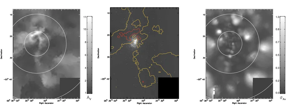
In this chapter we present a reconstruction of the OMC-1 extinction map based on the analysis of the NIR source catalog we compile in Chapter 1. In Sect. 2.1 we briefly review the previous studies relevant to the ON region. In Sect. 2.2 we illustrate our statistical method to disentangle background stars from the cluster population. By combining an estimate of the interstellar ex-tinction affecting each contaminant star with the source count density, we derive the OMC-1 extinction map. In Sect. 2.3 we apply a similar statistical proce-dure to the candidate cluster members, deriving an extinction map for the dust in the foreground ON. Finally, in Sect. 2.4 we compare our maps to previous studies, and we briefly discuss their main features and similarities to stellar distributions.
2.1
Overview of previous studies
A number of previous studies provide results relevant to the issue of the galactic reddening in the direction of OMC-1.
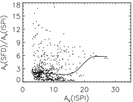
Schlegel et al. (1998) (SFD98 hereafter) combined the COBE /DIRBE ob-servations (100 µm and 240 µm) and the IRAS /ISSA obob-servations (100 µm) to obtain a full-sky 100 µm map with ∼ 6′
resolution. On the basis of the correla-tion between the Mg line strength and the (B − V ) color of elliptical galaxies, they were able to calibrate their column-density map to a E(B −V ) color excess map. Their all-sky reddening map, available through the NASA/IPAC Infrared Science Archive1 Dust Extinction Service web page, represents the benchmark
for the following studies of our region.
The accuracy of the SFD98 maps has been analyzed by Arce & Goodman (1999), who compared the extinction map of the Taurus dark cloud with the extinction maps obtained using four other methods, i.e. 1) the color excess of background stars with known spectral types; 2) the ISSA 60 and 100 µm images; 3) star counts; and 4) optical color excess analysis. These four methods give similar results in regions with AV ≤ 4. Their comparison shows that the
extinction map derived by SFD98 tends to overestimate the extinction by a factor of 1.3 ÷ 1.5. They ascribe this discrepancy to the the calibration sample of ellipticals used by SFD98, which containing few sources with AV > 0.5 may
lead to a lower estimate of the opacity. Arce & Goodman (1999) also find that when the extinctions shows high gradients (& 10m/deg, see their Fig. 1),
its value is generally smaller than that given from SFD98, and argue that the effective angular resolution of the SFD98 map could be somewhat larger than 6′
.
Dobashi et al. (2005) obtained another all-sky absolute absorption map applying the traditional star-count technique to the ”Digitized Sky Survey I” (DSSI) optical database, which provides star densities in the range ∼1– 30 arcmin−2. Comparing the SFD98 maps to their results in the Taurus,
Chameleon, Orion and Ophiucus complexes, they found that SFD98 extinc-tion values are generally up to 2-3 times larger (see their Figs. 46, 47 and 48). A least-squares fit of the two extinction estimates in the AV ≤4 gives a
propor-tionality coefficient of 2.17, while the same analysis in the AV ≥ 4 suggests a
coefficient of ∼ 3. The authors discuss the possible causes of discrepancy. First, they stress that the SFD98 map are mostly sensitive to the total dust along the line of sight, while their maps measure the extinction due to the nearby dust, as the optical thickness is much larger in the visible than in the far infrared. Sec-ond, they point out that the low resolution (∼ 1 deg) of the temperature map adopted by SFD98 cannot reproduce the typical high spatial frequency temper-ature variations across dark dense clouds. Finally, they suggest that SFD98 do not account for enhancement in the far infrared emission by fluffy aggregates: this excess emission could explain the inconsistency between SFD98 map and maps derived using other methods. Unfortunately, DSSI optical plates saturate in proximity of the Trapezium cluster, so a large fraction of the ONC field is excluded from their analysis.
An extinction map limited to the inner ∼5′
×5′
region of the ONC was pro-vided by Hillenbrand & Carpenter (2000) on the basis of the C18O column
den-sity data of Goldsmith et al. (1997), with a 50′′
spatial resolution. A comparison of the extinction map they derive with the extinction obtained by SFD98 shows that that the SFD98 extinction is generally ∼ 3 times larger.
In summary, the SFD98 extinction map for the OMC-1 is still the only one covering the entire ONC field. However, its spatial resolution (6′
) is limited and the accuracy, in a region as complex as the OMC-1, remains questionable.
In Sect. 2.2 we overcome most of the issues listed above using photometric data in the NIR bands, as they offer several well known advantages. First, 90% of the galactic population is made up of M dwarfs which, by virtue of their
2.2 The OMC-1 extinction map 40
Spectral Energy Distribution (SED), radiate mostly in the NIR. Second, the extinction is lower at IR wavelengths and therefore stars here can be more easily detected through optically thick clouds. Third, the high surface density of field stars allows to overcome the limited spatial resolution typical of far-infrared wide-field surveys used to measure diffuse dust emission. As a caveat, however, we anticipate that the number of detected background stars will be limited by the brightness of the background, which affects the completeness limit of the NIR survey (Sect. 2.2). This effect will be taken into account in our analysis.
2.2
The OMC-1 extinction map
To compute a new extinction map of the OMC-1 region, we use the NIR catalog we compile in Chapter 1. We concentrate our analysis on the (H,H-KS) CMD
of the ∼6000 point-like sources with both H and KS measured photometry.
Lombardi & Alves (2001) show that the inclusion of the J magnitudes can reduce the noise of the extinction measurements by a factor of two, especially in regions characterized by low extinctions. Unfortunately, this is not our case. By using the full sample of stars detected in the H and KS bands, we greatly
increase the stellar density and therefore maximize the angular resolution of our map, since our photometric catalog is shallower in the J-band. Our survey also lacks deep J-band observations of the North-East corner of their field, which makes the deep field covered by the the J-band smaller by about 9% than the field covered in H and KS-bands. Later in this chapter we will include the
J-band data, when we will consider the extinction map toward the ONC, which lays in the foreground of the OMC-1.
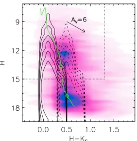
The (H,H-KS) CMD in Fig. 2.1 shows a characteristic bimodal distribution:
a first group of stars (the ONC) is clustered at H-KS=0.5 and H=12, whereas
a second group of fainter objects appears clustered around H∼17. This second group also has a peak, but this is a selection effect, as the number of faint sources drops at H&17.5 in correspondence of the sensitivity limit of our survey.
Figure 2.1 also shows a 2 Myr isochrone appropriate for the ONC (solid green line) and the density contour of the galactic stellar population along the line of sight of the ONC (solid contours). The galactic population has been derived from the Besan¸con galactic model (Robin et al. 2003)2, computed at
the galactic coordinates of the ONC over our survey area of 0.329 deg2. For