Amphipod assemblages of Posidonia oceanica meadows: space, time and metacommunity structure

UNIVERSITÀ DEGLI STUDI DELLA TUSCIA DI VITERBO DIPARTIMENTO DI SCIENZE ECOLOGICHE E BIOLOGICHE

CORSO DIDOTTORATO DIRICERCA IN

ECOLOGIA EGESTIONE DELLE RISORSE BIOLOGICHE- XXVII CICLO

A

P

:

,

TIME AND METACOMMUNITY STRUCTURE

(s.s.d. BIO/07)

Tesi di dottorato di: Dott.ssa Federica Camisa

Coordinatore del corso Tutor

Prof. Daniele Canestrelli Dott.ssa Roberta Cimmaruta

Co-tutor Dott.ssa Loretta Lattanzi

Dott. Bruno Bellisario

T

1. INTRODUCTION AND OBJECTIVES...1

2. BACKGROUND...3

2.1 Posidonia oceanica... 3

2.2 Amphipods... 8

2.3 Spatial/Temporal variation...13

2.4 Metacommunity... 18

3. MATERIALS AND METHODS... 29

3.1 Study area ... 29

3.2 Sampling methods ... 32

3.3 Statistical analyses... 35

3.3.1 Spatio-temporal analysis... 35

3.3.2 Pattern analysis...36

3.3.2.1 Commonness and rarity in community structure... 36

3.3.2.2 Elements of Metacommunity Structure... 37

4. RESULTS AND DISCUSSION...41

4.1 Seasonal fluctuations in amphipod communities associated with Posidonia oceanica meadows of Giannutri Island... 41

4.1.1 Results... 41

4.1.2 Discussion... 48

4.2 Spatial and temporal variation of coastal mainland vs. insular amphipod assemblages on Posidonia oceanica meadows... 53

4.2.1 Results... 53

4.3 Scale matters: the geographic insurgence of metacommunity structures in amphipods

of Posidonia oceanica meadows...65

4.3.1 Results... 65

4.3.2 Discussion... 70

5. CONCLUSIONS...75

1.

INTRODUCTION AND OBJECTIVES

Posidonia oceanica meadows represent a key ecosystem in the Mediterranean Sea, being a highly productive system able to supply a number of important ecosystem services. They play also an important role in marine food webs, by transferring organic matters from producers to first order consumers, and contribute to the maintenance of marine biodiversity by providing habitat for a large set of organisms that cannot live in unvegetated bottoms, such as vagile invertebrates. Among all, amphipod crustaceans represent an important component of the fauna associated with P. oceanica (Gambi et al., 1992). However, their ecology still remains partially unknown, as well as their impact on the functioning of seagrass meadows ecosystems, their feeding preferences and the role of spatial scales and environmental characteristic of habitats on their assemblage structure over time.

The general goal of this study is to deepen the knowledge of amphipod assemblages living on seagrass meadows by checking for their spatial and temporal variability (both on seasonal and annual basis) and the emergence of metacommunity patterns. To achieve this goal, we studied the amphipod assemblages on P. oceanica meadows during two consecutive years from three different localities in central Tyrrhenian Sea at increasing spatial distance. To reach this objective, the research was subdivided in three tasks.

1. The first task was aimed at analyzing the spatial and temporal variability of amphipod assemblages in P. oceanica meadows from insular vs. mainland coastal areas. Diversity and multivariate analyses were used to investigate the role of direct and

indirect effects of space in the patterns of amphipod distribution within seagrasses. To this end, two sampling localities were chosen in close proximity along the northern coasts of Latium (Central Italy), characterized by high anthropogenic disturbance, which is responsible for eutrophication and turbidity of coastal waters (Paganelli et al., 2013). Amphipod assemblages of these two mainland localities were compared with those from Giannutri Island, a Marine Protected Area belonging to the National Park of Tuscan Archipelago. The temporal variability of assemblages in three study localities was also investigated by analyzing their composition across two years (summer 2012 and 2013).

2. The second task aimed at analyzing the structure and yearly seasonal variability of amphipod communities from two localities of Giannutri Island (Punta Secca and Secca di Punta Secca). Diversity and multivariate patterns of assemblages were used to evaluate the role of spatial vs. seasonal factors in structuring P. oceanica amphipods during one year of sampling. Further analyses were carried out in order to shed light on the number and identity of species influencing the seasonal dynamics. A further contribution of this task was to deepen the knowledge of the benthic fauna of Giannutri Island, which was previously lacking.

3. The third task was aimed at understanding whether and how the amphipods-Posidonia system can be considered as a metacommunity. In particular, we tested for the existence of a spatial scale at which patterns of metacommunity structure emerge, and if these scales are conservative in time. The ultimate aim of this task was to provide a rigorous statistical approach able to measure the geographic extent at which regional, dispersal-based processes surpass the local, niche-based ones in explaining the pattern of biodiversity in amphipods-seagrass systems.

Recent findings in conservation biology showed the need to understand patterns of biodiversity in a spatial context, focusing on the dynamic responses of habitat loss at landscape level (i.e. the secondary loss of biodiversity, Cabeza and Moilanen, 2001). Anthropogenic alterations may indeed act at different spatial scales, ranging from local to regional and global, so that a metacommunity perspective becomes fundamental to assess the relative importance of spatial and environmental components in the variability of community assemblages (Heino, 2013).

Peracarid crustaceans are widely used as sensitive indicator of marine environmental alterations (Bellan-Santini, 1980; Conradi et al., 1997), but their responses may be strongly influenced by the spatial heterogeneity of the meadows (Stoner, 1980a, 1980b; Parker et al., 2001), the spatial scale of observations and the fluctuation of the environmental characteristic of habitats over time. We believe that our approach may be useful to test a series of theoretical and conservation issues, providing an insight into the patterns, scales and processes involved in the responses of the amphipods metacommunity to the main structuring processes.

2.

BACKGROUND

2.1 Posidonia oceanica

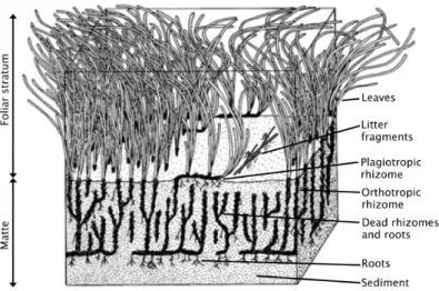
The seagrass Posidonia oceanica is a marine phanerogam belonging to the group of angiosperm monocotyledons. The genus Posidonia includes about 60 species among which the widespread Mediterranean species P. oceanica, Zostera noltii, Cymodocea nodosa, Halophila stipulacea and Nanozostera noltii. Being a vascular plant P. oceanica maintained characteristics similar to those of terrestrial plants, such as the

structure differentiated into roots, rhizome (modified stem) and leaves (Fig. 2.1), and sexual reproduction with flowering.

Figure 2.1 - Schematic representation of the structure of a Posidonia oceanica meadow).

P. oceanica is the most important seagrass species in the Mediterranean area, where it is almost ubiquitous covering 2% of the seabed and colonizing areas less exposed to hydrodynamism (Garcia and Duarte, 2001; Lipkin et al., 2003; Procaccini et al., 2003). It settles mainly on sandy bottoms, but can also colonize irregular substrates and rocky seabeds at a variable depth between less than 1 m up to a maximum of 40 m. The upper limit depends mainly from the intensity of hydrodynamism, while the lower limit is influenced by both light availability and water transparency (Boudouresque et al., 2006).

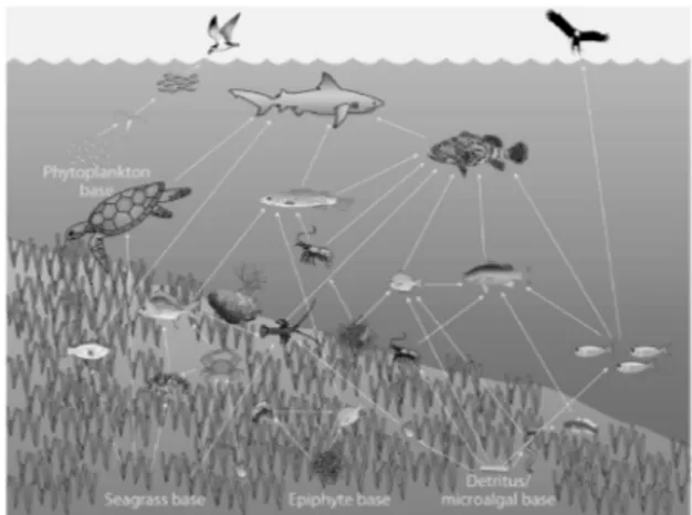
Besides its extension, P. oceanica meadows represent a key ecosystem and play one of the most important ecological roles in the Mediterranean coastal area, being listed among priority habitats (1120*_{) in the Habitats Directive (92/43/EEC). P. oceanica}

such as providing nursery habitat, refuge from predators and representing a direct or indirect source of food for many species (Fig. 2.2) (Macpherson et al., 1997; Cebriàn and Duarte 2001; Guidetti, 2000).

Figure 2.2 - Scheme of a marine trophic web associated with seagrass.

As a consequence, it has a relevant ecological importance as ‘foundation species’ because it defines much of the structure of local communities by creating locally stable conditions for other species, by modulating and stabilizing fundamental ecosystem processes (Dayton, 1972). P. oceanica forms meadows that occur as a continuum of many plants able to mitigate the wave energy, with the leaves favouring the sedimentation of suspended particulates and protecting from coastal erosion. P. oceanica plays a key role in the food web due to its ability to maximize the amount of biomass produced with respect to the energy flow, a strategy that allow to enhance the ecosystem’s resilience (Boudouresque et al., 2006).

Examining the characteristics of the meadows and associated populations allows to assess the health status of the ecosystem, so that P. oceanica has been selected as a

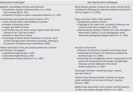
bioindicator of Mediterranean coastal waters quality due to its wide distribution and sensitivity to sources of human disturbance. P. oceanica is extremely sensitive to various kinds of disturbance, despite it is able to establish stable and long-lived systems under undisturbed conditions (Duarte, 1991; Di Carlo et al., 2007). Under both natural (e.g. Pleistocenic climate changes) and human impacts, the regression of the meadow occurs over both small or large scale, usually affecting the superficial zone of the prairie, more exposed to the pressure exerted by human activity and, therefore, more vulnerable (Pérès and Picard, 1975; Bourcier, 1989; Peraino and Bianchi, 1995; Marbà et al., 1996; Boudouresque et al., 2009). Among the main impacts affecting P. oceanica meadows it can be listed the trawling, which destroys the meadows at large scale, all sorts of pollution, including sewage, dumping and oil spills, introduced species and, finally, moorings, dredging and any infrastructure altering the physical characteristics of the environment (Meinesz et al., 1991; Guidetti and Fabiano, 2000; Badalamenti et al., 2006). This latter, in particular, may reduce the hydrodynamic regime, causing an excess of sedimentation that results in a ‘choking’ of P. oceanica. Aquaculture activities can also impact P. oceanica meadows (Pusceddu et al., 2007), by increasing the supply of organic material at the bottom, in the adjacent areas and in the water column, reducing water transparency and limiting the photosynthetic capacity of plants with consequent decrease in biomass and density (Pusceddu et al., 2007). A series of different methodologies, listed in Table 2.1, may thus be performed in order to assess the health status of the meadows in Mediterranean area.

Table 2.1 - The analyses on Posidonia oceanica most routinely employed by the Mediterranean research laboratories, separated in destructive and not destructive techniques (from Montefalcone, 2009)

Given the major role played by P. oceanica in Mediterranean coastal ecology, the regression of the meadows may affect many aspects of the associated community structure, which is moulded by the interactions between the plant, the epiphytes and the animals through processes of co-evolution. Environmental gradients, such as the intensity of hydrodynamics and the temperature, are the driving force that influence, directly and indirectly, the algal fraction (along the layer leaf) and animal community (Mazzella et al., 1989). Changes in environmental parameters can determine differences in the structure of the meadows and, consequently, in the structure and distribution of the community.

The assemblages associated with P. oceanica vary on a geographic, seasonal and bathymetric scale, but some species are constantly present throughout the Mediterranean. P. oceanica habitats are characterized by extremely high levels of

biodiversity. A fundamental contribution to the high biodiversity of P. oceanica system is given by the epiphytic community (Klumpp et al., 1992; Moncreiff et al., 1992; Nelson and Waaland, 1997), characterized by a great variability over a small spatial scale (form cm to m) and by a greater uniformity over large-scale (km), thus showing a patchy distribution (Balata et al., 2007). The epiphytic flora contributes to the overall primary production system of P. oceanica (Cebriàn and Duarte, 2001; Romero, 2004; Boudouresque et al., 2006), furthermore representing the main source of food for most of herbivores associated with seagrass meadows (Fig. 2.2). Another fundamental component in the P. oceanica ecosystem is the vagile fauna (Kikuchi and Pérès, 1977), which includes all of the associated organisms free to move independently although being sedentary. The vagile fauna show a zonation along the depth gradient and in relation to seasonal variation, with a distribution that is the result of adaptation to abiotic conditions, thus reflecting the presence of environmental gradients (Mazzella et al., 1989, 1990; Gambi et al., 1992). The main taxonomic groups of vagile fauna associated with P. oceanica meadows are molluscs, polychaets, annelids, echinoderms and crustaceans. Among the latter amphipods predominate, representing one of the most abundant taxonomic group (Marsh, 1973; Mazzella and Russo, 1989).

2.2 Amphipods

Amphipods, with more than 8,000 described species (Bellan-Santini, 1999), are the most numerically important order inside the superorder of Peracarid Malacostraceans Crustaceans, whose phylogeny remains to a large extent an unresolved mess with the possibility that it may be a polyphyletic group (Martin and Davis, 2001). The

subdivision of amphipods is constantly debating, but traditionally they are subdivided in four sub-orders: Gammaridea (maybe paraphyletic and contain the vast majority of amphipod families), Caprellidea (strictly marine, with a peculiar morphology), Hyperiidea (exclusively planctonic, characterised by important development of the eyes), and Ingolfiellidea (interstitial, with a lower species diversity) (Barnard and Karaman, 1991).

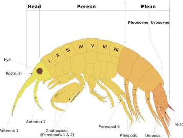
Amphipods exhibit a variety of different morphologies but all have certain basic features. The general ‘type amphipod’ is a small crustacean (about 10 mm), with an arched, laterally flattened body (Fig. 2.3) that can be divided in three main parts. The head is a cephalothorax resulting by the fusion of the head with the first thoracic segment. It bears a pair of sessile compound eyes, two pairs of uniramous antennae and three pairs of mouthparts (mandibles and two pairs of maxillae). The first thoracic segment bears the maxillipeds, prehensile appendages involved in food handling (Bellan-Santini, 1999).

The thoracic part, called pereon, includes seven segments each of them bearing a pair of pereiopods consisting of seven articles: the coxa, the basis, the ischium, the merus, the carpus, the propodus and the dactylus. The first four pairs of pereiopods are pointed towards forwards and the last four pairs backwards, a peculiar feature that gives its name to the order, ‘amphi-’ meaning ‘both’ and ‘poda’ meaning ‘foot’ or ‘leg’ (Bellan-Santini, 1999). The pereiopods of the first two segments are modified to be prehensile appendages and take the name of gnathopods (‘gnato-’ mening ‘jaw’ combined with ‘poda’), while the other five pairs are adapted for locomotion. In most cases, each of the pereiopods of the 6 last segments bear gills. They have separate sexes and some species present accentuated sexual dimorphism (Riedl, 2010). In mature females, the coxa of pereiopods can present a large ventral lamellar projections, called oostegites, that participate in the formation of the thoracic marsupium, a mid-ventral brood pouch characteristic of all peracarids. Breeding takes place with external fertilization, the female’s marsupium hosts the fertilized eggs and subsequent larval stages, then young amphipods are released in the environment under the form of juveniles that are morphologically close to adults (Barnard and Karaman, 1991), so that amphipods completely lack a dispersal larval phase (direct development). Mediterranean amphipods species show a rapid growth and a relatively short life in the range of 4-6 months up to 2 years (Bellan-Santini, 1998, 1999; Delgado et al., 2009).

Pleon is the abdominal part, composed of the last 6 segments of the body. It can be divided in two parts: the pleosome, (or epimeron), constituted of 3 segments (the epimers) each bearing a pair of pleopods used for swimming, and the urosome also contains 3 segments, each of them bearing a pair of appendages (uropodes), which are

very variable in shape and sometimes involved in the mating process. The final segment is the telson, which is can be a single plate, or partially or totally divided into two lobes (Bellan-Santini, 1999).

Amphipods inhabit a variety of different environments, including rivers, ponds, lakes, interstitial or underground waters, coastal marine environments, abyssal trenches and hydrothermal vents. Some of them are terrestrial forms and others are able of various symbiotic associations with vertebrates and invertebrates. This habitat diversity is correlated with an high diversification in the feeding type with herbivores, suspension or deposit feeders, scavengers, parasites, predators, detritivores, etc... (Bellan-Santini, 1999). This important adaptive radiation led the amphipods to become one of the dominant groups of marine invertebrates in numerous ecosystems. The large number of species and their wide dissemination, as well as the variety of ecological niches occupied by different species led the amphipods to become one of the dominant groups of marine invertebrates and puts them in a position to be used in the field of ecological indicators. Amphipods are particularly sensitive to polluted sediments showing an overall decline in the abundance and diversity in species with increasing pollution (Gómez-Gesteira and Dauvin, 2000; Dauvin and Ruellet, 2007) and, therefore, used in monitoring the environmental impacts on the prairies themselves (Sánchez-Jerez and Ramos-Esplá, 1996; Sánchez-Jerez et al., 2000).

Vagile invertebrates, in particular amphipods, are often regarded as key-components of seagrass systems because of their importance in food webs. The knowledge about their trophic ecology is still poor, but amphipods are generally considered to be primary consumers and/or detritivores constituting an important link between producers and higher trophic levels. Amphipods are mainly generalist herbivores, feeding vegetal

epiphytes (diatoms and macroalgae) and associated detritus on the leaves, but some are deposit/suspension feeders, omnivores, deposit feeders, carnivores and detritus feeders (Gambi et al., 1992; Lepoint et al., 2000; Vizzini et al., 2002)

Epiphyte-derived organic matter has a relevant importance in the diet of amphipods associated with P. oceanica meadows, which consume epiphyte growing on various parts of the seagrass, with species-specific preferences (Mazzella et al., 1992), making the organic matter constituting them available to upper trophic levels and so holding a central role in the food webs associated with P. oceanica meadows (Bell and Harmelin-Vivien, 1983; Pinnegar and Poulin, 2000). For these reasons, abundance of leaf epiphytes is an important factor driving the patterns of amphipod community structure (Zakhama-Sraieb et al., 2011).

In seagrass meadows, the seagrass, the epiphytes that grow on it and the grazers able to consume either the seagrass or its epiphytes are linked by a complex interplay of reciprocal interactions, termed seagrass/epiphyte/grazer system. Fluctuations in this system can influence the functioning of the whole meadow (Jernakoff et al., 1996; Valentine and Duffy, 2006) and amphipod crustaceans, because of their great abundance, could play an important role in the determination of the structure of the community (Connell, 1975).

P. oceanica meadows exhibit a higher numerical abundance and specific diversity of amphipods than unvegetated sand bottom areas, showing differences also from communities found in other common soft-bottom Mediterranean macrophytes (Scipione and Zupo, 2010). Although the amphipods fauna associated with P. oceanica is rich and

particular, with a lot of species considered, real exclusive taxa of this biotope do not exist (Buia et al., 2000).

The meadow-associated community can be regarded as a complex assemblage of species that may be encountered also in other biotopes. The fauna of the foliar stratum is very similar to biocenoses encountered in photophilous algae on rocky shores, while the fauna of the rhizome layer matte is comparable to the fauna of precoralligene and coralligene bottoms, or marine caves. Finally, communities of the matte show similarity with those associated to sediment on detrital soft bottoms (Ruffo et al., 1989). Such distinction is, however, unclear because of the ability of this animals to perform vertical migrations creating interaction between the different compartments and causing a partial overlap of the assemblages (Borg et al., 2006).

2.3 Spatial/Temporal variation

Posidonia oceanica meadows are habitats characterized by a high spatial heterogeneity and variability even over small scales, ranging from meters to centimeters (Balestri et al., 2003; Borg et al., 2005, 2006; Montefalcone et al., 2008; Sturaro et al., 2014, 2015). Factors that could modify the morpho-functional traits of the plants include physical disturbance, topographic complexity, nutrient availability as well as differences in microhabitats. Such factors may operate over very small scales, thus altering plants distributional patterns over comparable distances (cm to dozens of m), and so causing the well documented high spatial heterogeneity of meadow features (Balestri et al., 2003; Zupo et al., 2006a, 2006b).

P. oceanica system is also characterized by a certain degree of seasonally-based variability, as observed in many other long-lived seagrasses with large-sized rhizomes (Duarte, 1991). Their ability in storing and reallocating resources allows the plants to support growth patterns that are relatively independent from fluctuating environmental conditions, but prone to be influenced by changing seasons (Marbà et al., 1996; Guidetti et al., 2002). Leaf area index and shoot weight (see Table 2.1) reach their maximum during late spring and summer, when both the foliar production of P. oceanica and the development of epiphytes are higher (Guidetti et al., 2002). During these periods, litter constantly accumulates, especially via erosion of the apexes of the leaves due to the heavy epiphytic load and associated grazing activities. At the beginning of the autumn the significant development of epiphytes together with the increasing hydrodynamism, both contribute to the massive fall of senescent leaves (Guidetti et al., 2002). During the late autumn and winter, most of the litter is degraded or exported, albeit not immediately renewed due to the lowered productivity of P. oceanica (Mateo and Romero, 1997; Gobert, 2002; Gallmetzer et al., 2005).

Seagrass meadows are spatially heterogeneous ecosystems, where a number of microhabitats coexist, creating intricate structures that favour a patchy distribution of associated invertebrates. Effective conservation and management of seagrass communities thus require a clear understanding of the processes controlling the patterns of distribution of associated organisms, with particular regard to the variation in species abundance and diversity through space and time. Temporal and spatial variation of the structure of P. oceanica meadows, as the leaf canopy height and shoot density (Table 2.1), are key drivers in determining spatial and temporal patterns of distribution, therefore influencing species richness and abundance of the leaf-stratum-motile macro

invertebrate assemblages (Bedini et al., 2011; Michel, 2011). Canopy height and shoot density are related to both habitat complexity and availability of different microhabitats, influencing food availability for grazers, in terms of epiphyte abundance, enhancing the role of meadows as refuges from predation (Mazzella and Ott, 1984; Borg et al., 2010). Associated vagile fauna is therefore strongly influenced by the features of both the plant and of its epiphytes, showing specific adaptations to different micro-environments (Mazzella and Ott, 1984).

Among all, amphipods are one of the most important components of the P. oceanica vagile fauna (Ledoyer, 1962; Mazzella et al., 1989), playing a relevant role in the transfer of energy to the higher trophic levels and represent an important source of food for higher trophic levels, as decapods and fishes (Bell and Harmelin-Vivien, 1983; Chessa et al., 1983; Sparla, 1989). Depth is advocated as fundamental in the subdivision of amphipods, and studies on the bathymetric variation suggest that communities are structured in 3 assemblages. The shallow water community, located between the surface and 1-2 m depth, is very similar to the photophilous algae fauna. Such assemblage is able to withstand high hydrodynamism and is mainly represented by herbivores related to the erect algal epiphytic layer, which constitutes the primary food source for amphipods. The intermediate amphipod community ranges from 5-10 m to 20-25 m depth, and is characterized by a more diversified assemblage that is considered the most typical of P. oceanica meadows. It is mainly represented by herbivores-deposit feeders, due to the high deposition of particulate organic matter on leaves that may favour the presence of ‘detritus cleaner’ species (Nagle, 1968; Howard, 1982; Lewis and Hollingworth, 1982; Scipione, 1989). Finally, the third assemblage is found at depths higher than 25 m, and is similar to the amphipod assemblages found in bare soft

bottoms, characterized by a preponderance of deposit-suspension feeders and deposit feeders-carnivores. These features are probably due to the more heterogeneous structure of the meadows and the overlapping with surrounding soft bottoms (Scipione and Fresi, 1984; Mazzella et al., 1989; Gambi et al., 1992; Michel, 2011). This bathymetric pattern of distribution is often related to the trophic structure of assemblages: higher food availability could explain a higher abundance of herbivorous organisms in shallow stands, while carnivorous organisms may colonize the deeper parts of meadows (Mazzella et al., 1992).

Studies on spatial variation of amphipod assemblages have been carried out in meadows from Spain (Sánchez-Jerez et al., 2000; Vazquez-Luis et al., 2009), continental French (Ledoyer, 1968), Corsica (Degard, 2004; Sturaro, 2007), Sardinia (Como et al., 2008; Sturaro, unpublished data), Italian Tyrrhenian coasts (Scipione and Fresi, 1984; Chimenz et al., 1989; Mazzella et al., 1989; Gambi et al., 1992; Scipione et al., 1996), Italian Adriatic coasts (Scipione and Zupo, 2010) and Tunisia (Zakhama-Sraieb et al., 2006; Zakhama-Sraieb et al., 2011). These studies have evidenced that, while common features can be highlighted, it is difficult, if not impossible, to evidence a general pattern (Michel, 2011). Most of the variability in the total abundance, specific diversity of communities and identity of dominant species could be probably explained by local differences of the meadow parameters.

Moreover, many studies suggest that spatial variation could exist at very small scale (e.g. 1-10 m) (Gambi et al., 1992; Sánchez-Jerez et al., 1999a; Degard, 2004; Zakhama-Sraieb et al., 2011), while variations at larger scales (about 100 m) rather concern amphipod specific richness and diversity (Sturaro, 2007). Motile macro-invertebrate assemblages associated with seagrasses may vary spatially in relation to responses of

organisms to environmental gradients and, temporally, in relation to the life cycle of organisms and changes in the structure of seagrass beds (Heck and Orth, 1980). Temporal variation can also be considered scale dependent, particularly in the case of motile animals such as amphipods, the situation is further complicated by vertical (nychthemeral) and horizontal migration patterns.

Nychthemeral variation is an important pattern of movement, showing an increasing abundance of amphipods in the foliar stratum during the night (Ledoyer, 1969; Sánchez-Jerez et al., 1999b). Such pattern of migration is likely explained by the greater nocturnal activity of amphipods (Bellan-Santini, 1999), described as a mechanism of predation avoidance. A large number of predators of the vagile invertebrates are fish (e.g. Labrus merula, Symphodus rostratus), which mostly feed during the day and hunt their preys using visual stimuli (Bell and Harmelin-Vivien, 1983). Like other groups of vagile invertebrates, amphipod crustaceans developed mechanisms of vertical migration as a strategy to avoid this kind of predation. During the day, they preferentially stay in the lower layers of the meadow (rhizomes, matte, Ledoyer, 1969), rising to the foliar stratum (where they are more vulnerable) only during the night when the predation pressure is lower (Ledoyer, 1969). Moreover, these vertical migrations could limit the competition for food or habitat, by allowing animals to exploit available resources in all compartments (foliar stratum, rhizome layer and litter cover) (Sánchez-Jerez et al., 1999b).

Important seasonal influences on the spatial distribution of invertebrates within the meadows may also exist (Bedini et al., 2011). Amphipod abundance and diversity is generally maximal in late summer and autumn and minimal in winter and early spring (Mazzella et al., 1989; Gambi et al., 1992; Scipione et al., 1996). Specific traits of the

meadow often cannot explain such variability so that the autumnal maximum can be linked to seasonal differences of other abiotic and biotic factors, like lower predation pressure and individual dynamics of vagile invertebrates (Nelson, 1979a, 1979b; Michel, 2011; Michel et al., 2014). Other sources of variability in the temporal patterns of abundance of motile fauna are related to temporal changes in epiphyte diversity and covering. Herbivores, probably, follow the seasonal changes of epiphyte biomass and the abundance of carnivorous assemblages would vary less over a one-year period (Mazzella et al., 1992). Long-term temporal variation could also occur, but the different seasonal distributions of dominant species within the same trophic group are most likely due to different life cycles, competition phenomena, or various grazing adaptations to plant epiphytes (Greze, 1968).

2.4 Metacommunity

The knowledge of distribution and abundance patterns of species is fundamental to understand the role of biodiversity in ecosystem functioning (e.g. maintaining water quality, atmospheric CO2 levels, or primary production; Loreau, 2000; Naeem, 2001;

Holyoak et al., 2005). Biodiversity is structured by processes operating at several hierarchical scales, including populations of single species, interacting populations of different species, whole communities and ecosystems. Patterns of biodiversity are innately spatial, scaling from local ecosystems to landscapes to entire biogeographic regions (e.g. Wiens, 1989; Levin, 1992; Holt, 1993; Rosenzweig, 1995; Maurer, 1999; Hubbel, 2001; Chase and Leibold, 2003). Of particular interest are cases where patterns

of diversity are linked to changes in community composition along environmental gradients.

During the last years, ecologists have increasingly questioned whether the existing conceptual framework of community ecology is adequate for describing the dynamics of communities that are connected across space. The metacommunity concept has emerged as a new and exciting way to think about spatially extended communities, leading novel questions about emergent patterns of species diversity and distribution. A metacommunity can be defined as a set of local communities that are linked by dispersal (Hanski and Gilpin, 1991; Wilson, 1992), where a community may be defined as a collection of species occupying a particular locality or habitat. These definitions describe a hierarchy of scales and emphasize the ways in which processes occurring at smaller scales interact with those at larger scales (Levins and Culver, 1971; Vandermeer, 1973; Crowley, 1981; Law et al., 2000; Mouquet and Loreau, 2002).

A motivation for studying metacommunities comes from the need to conserve biodiversity in landscapes experiencing fragmentation. Habitat fragmentation creates patchy landscapes in which dispersal may be required for persistence, and is acknowledged to be an important factor driving the loss of biodiversity (Wilcove et al., 2000). Fragmentation studies typically use empirical trends to predict how communities will change during fragmentation process, investigating the ability of species traits to predict responses to fragmentation itself.

However, such studies rarely attempt to explicitly deal with community structure due to the lack of a general theory framing the measures and analyses of natural fragmented communities. In single species metapopulation models, the subdivision of the habitat

resulting from fragmentation can only be detrimental because, as fragmentation proceeds, previously stable populations in large undivided habitats become increasingly small and isolated. This makes them vulnerable to local extinction through demographic stochasticity, with a reduced capacity for the patches to be recolonized (Harrison and Taylor, 1997). The absence of a theory able to provide mechanisms for responses to fragmentation potentially limits our ability to predict how communities will change under altered circumstances and our ability to effectively manage communities and metacommunities by manipulating habitat factors al landscape scales. These substantial gaps in the knowledge require a clear understanding of the role of spatial structure and dynamics in ecological communities to maintain biodiversity, to manage species and ecosystem properties and to provide adequate practices in conservation biology.

A community is often defined as an area within which all individuals are equally likely to interact, precluding any spatial heterogeneity in distribution or abundance. This simplified view assumes that mass action and mean field conditions are adequate descriptors of the dynamics, as seen in population dynamic models such as the classic Lotka-Volterra equations and their extensions (May, 1973; Pimm and Lawton, 1978; McCann et al., 1998). It is also often not clear whether the results of these investigations are applicable in all generality to more complex systems at larger spatial scales (Naem, 2001).

A metacommunity is easiest to conceptualize when all the interacting species utilize the same set of discrete habitat patches and have local populations that use resources at the same within-patch scale. However, many communities lack discrete boundaries, and many populations are regulated over multiple spatio-temporal scales. In addition, the exact spatial placement (i.e. spatially explicit) of habitats can influence metacommunity

dynamics, so that species can differ in the extent to which they disperse. Inter-patch dispersal at sufficiently low rates can lead to variation in species composition from patch to patch. Although existing models of metacommunities (Hubbell, 2001; Mouquet and Loreau, 2002, 2003) give a highly simplified representation of the spatial complexity of natural assemblages, they are useful in developing theories for more complex metacommunity scenarios. Metacommunity dynamics consist of either the spatial dynamics or regional properties of communities occupying two or more interconnected patches. In contrast to metapopulation dynamics, metacommunity dynamics should involve more than two interacting species. Differently from community dynamics, the metacommunity concepts should be applied to a system in which the dynamics of individual species were altered by both species interactions (of more than two species) and dispersal. Variation in the extent to which species interact has profound consequences for metacommunity dynamics. Dispersal may influence both local and regional dynamics, with different species likely to have their own rates of movement that represent a combination of evolved abilities and responses to their environment (Holling, 1986; Clobert et al., 2001; Rodrìguez 2002).

The number of spatial scales that are required to represent the dynamics of real metacommunities is not yet clear. Many current models of metacommunity dynamics are based on a three-level hierarchy of scales. At the smallest scale, micro-sites can hold a single individual and are nested within localities (equivalent to habitat patches) that hold local communities similar to those in conventional species interaction models. In turn, local communities are connected to other communities as part of a metacommunity occupying a region. Not only the number or the extent, but also the real arrangement of patches/localities (i.e. the so called spatially explicit models) should be considered in

explaining metacommunity patterns, as ignoring explicit spacing may led a too simplified view of the reality (Hanski and Gaggiotti, 2004).

Four conceptual models can be considered to describe metacommunities, and each one illuminates different aspects of spatial community dynamics. Theoretical and empirical work on metacommunity largely falls along four broad perspectives that we refer to as the patch dynamic, species sorting, mass effects and neutral perspectives. The first perspective (patch dynamic) extends metapopulation models for patch dynamics to more than two species, and it can be considered to build on the equilibrium theory of island biogeography (MacArthur and Wilson, 1967). Patch dynamic assumes the existence of multiple identical patches (e.g. islands) that undergo to both stochastic and deterministic extinctions (Harrison and Taylor, 1997). Under this view, dispersal should counteract extinctions by providing a source of colonization into empty patches. For coexistence to occur, dispersal rates must be limited so that dominant species cannot drive their competitors or prey to regional extinctions. The equilibrium theory of island biogeography also assumes a prominent role for extinction and colonization in setting levels of biodiversity on islands: species from a fixed pool of mainland species randomly colonize islands (patches), so that mainland species diversity determines the regional species diversity. However, such a perspective is not always realistic because many systems do not have a large mainland with a fixed species composition. Indeed, the equilibrium theory of island biogeography considers only the number of species in a community and does not include community (trophic) structure, species identities, or niche differentiation (Chase and Leibold, 2003).

The second approach (species sorting perspective) is based on theories of community change over environmental gradients (Whittaker, 1972), and considers the effects of

local abiotic gradients on the population vital rates and species interactions (Leibold, 1998). The ensemble of local patches is heterogeneous in some local factors, and the outcome of local population dynamics (species interaction and individual species responses) depends on these spatially varying aspects of the abiotic environment. This perspective has much in common with traditional theory on niche separation and coexistence (Dobzhansky, 1951; Pianka, 1966; MacArthur and Levins, 1967). The main differences are that, under the metacommunity perspective, local and regional mechanisms of coexistence are intimately linked, and about the role of regional diversity in making local communities appear saturated. The result is that species distributions are closely linked to local conditions and are largely independent of unrelated purely spatial effects (Leibold and Norberg, 2004). Patch dynamic and species sorting perspectives assume a separation of time scale between local dynamics and colonization-extinction dynamics, but important regional dynamics may also emerge when local population dynamics are quantitatively affected by dispersal.

The mass effect perspective (Shmida and Wilson, 1985) represents a multi-species version of source-sink dynamics (Holt, 1985, 1993; Pulliam, 1988) and rescue effects (Brown and Kodric-Brown, 1977). Differences in the population density at different locations (or asymmetric dispersal) can drive both immigration and emigration between local communities. Immigration can supplement birth rates and enhance the densities of local populations beyond what might be expected in closed communities, and emigration can enhance the loss rates of local populations. Such ‘mass effect’ due to dispersal can have potentially strong influence on the relationship between local conditions and community structure (Holt, 1993). Coexistence in such a metacommunity is obtained through a regional balance of local competitive abilities and,

as a consequence, species are locally different but regionally similar in their competitive abilities (Mouquet and Loreau, 2002). The way with which mass effect allows the local coexistence of species is constrained in complex ways (Amarasekare and Nisbet, 2001) as coexistence requires spatial variance in fitness, which cannot be maintained at high levels of dispersal among patch types.

All of the above approaches assume that species differ significantly from each other either in their niche relations with local factors and/or in their abilities to disperse or avoid local extinctions. In the absence of any such differences among species, the behaviour of metacommunities can be dramatically different from models with trade-off or species-specific differences (Caswell, 1978; Hubbel, 2001; Chave, 2004). Neutral models predict a gradual loss of all competing species via a potentially slow process of random walks. The resultant temporal change in species composition has termed ecological drift by Hubbel (2001). Although neutral model, alone, cannot explain how differences in local and regional diversity are maintained, the ‘neutral’ view can be regarded as a null hypothesis for the other three views described above (Bell, 2000), able to describe the dynamics of communities where species are close to being equivalent, or where transient dynamics are very long.

Clearly, all of four perspectives outlined above capture interesting aspects of metacommunity dynamics. However, it is unlikely that all of the species interacting in a given (meta)community will uniformly conform to any one of these perspectives and, therefore, should be viewed as a continuum where each processes will play interactive roles in structuring real metacommunities. Moreover, many other factors not included in these four perspectives are likely to influence metacommunity dynamics, such as local dynamic or the evolution of species pool (Shurin et al., 2000). Such identified

paradigms should indeed be viewed as a starting point, rather than a complete framework, for metacommunity ecology.

The metacommunity concept advanced understanding of meso- and large-scale ecology, as well as the distribution of organisms along environmental gradients (Holyoak et al., 2005; Presley et al., 2010). Spatial variation in species composition can be studied by following complementary avenues based on mechanisms (Cottenie, 2005) and patterns (Leibold and Mikkelson, 2002). In the first approach (mechanistic), variation in community composition at different localities is based on the above mentioned paradigms of patch dynamics, species sorting, mass effects and neutrality (Leibold et al., 2004; Holyoak et al., 2005). A different but complementary approach in studying metacommunities is the evaluation of how species distribute along environmental gradients, emerging from the above mentioned mechanisms and manifest as particular metacommunity structures.

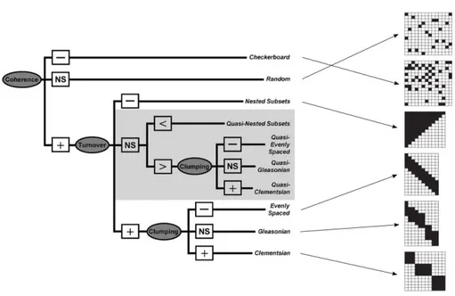
Several conceptual models of spatial structure have been developed to describe patterns of species distribution, each one based on the coherence of the species responses to environmental gradients and species turnover. To distinguish multiple hypothetical patterns, Leibold and Mikkelson (2002) developed a rigorous quantitative approach based on species incidence matrices, describing the presence/absence of a species in a given site. The approach of Leibold and Mikkelson (2002) is based on the assumption that most of underlying structures in metacommunities can be described by three elements, that is, coherence, range turnover and range boundary clumping. These elements, in turn, give six idealized structures (e.g. random, checkerboard, nested, evenly-spaced, Gleasonian and Clementsian) (Fig. 2.4), assuming that species distribution are molded by interactions (e.g. competition, habitat associations) or

responses to abiotic factors (e.g. temperature, rainfall) that vary among sites and so constitute an environmental gradient (Leibold and Mikkelson, 2002; Presley et al., 2010).

Figure 2.4 - Framework representing the hierarchical approach based on analysis of Elements of Metacommunity Structure and combinations of results that are consistent of each of six idealized structures (Leibold and Mikkelson, 2002), three patterns of species loss for nested subsets, six quasi-structures, and structures of compartments within Clementsian distributions.

The idealized patterns of species distribution are laying their foundations on early theories of species coexistence. For instance, Clementsian patterns are based on communities with distinctive species compositions sharing evolutionary history, but having interdependent ecological relationships. This results in boundary ranges that are coincident and form a sort of compositional unity along different parts of the environmental gradient (Clements, 1916). Alternatively, species may exhibit idiosyncratic responses to the environment, with coexistence resulting from chance similarities in requirements or tolerances (Gleason, 1926). Moreover, in presence of

strong interspecific competition, coexistence may be controlled by tradeoffs in competitive abilities, with species distributions that are more evenly spaced along environmental gradients than expected by chance (Tilman, 1982). Strong competition may also results in checkerboard patterns, when pairs of species have mutually exclusive ranges (Diamond, 1975) and occur at random with respect to other such pairs. Finally, nested patterns arise when species-poor communities are subsets of increasingly more species-rich communities (Patterson and Atmar, 1986), where species loss is associated with variation in species-specific characteristics (e.g. dispersal ability, habitat specialization, tolerance to abiotic conditions).

This theoretical framework has found its practical application in the Elements of Metacommunity Structure (EMS), which is based on the evaluation of the above mentioned structures calculated from a presence-absence interaction matrix, with sites as rows and species occurrences at sites as columns (Dallas, 2014). In this framework, the interaction matrix is first ordered via Reciprocal Averaging (RA), a multivariate ordination method that groups interactions along the matrix diagonal resulting in species with similar ranges and sites with similar species compositions to be placed together (Gauch, 1982; Dallas, 2014). The peculiarity of RA is that sites and species are ordered following latent (environmental) gradients and the scores of the resulting ordination can be related to environmental or spatial variables (Presley and Willig, 2010). However, incidence matrix can be ordered by following any relevant ecological questions.

Coherence is thus measured as the number of embedded absences in the ordered matrix, whose statistical significance is evaluated by comparing the observed absences to the number of embedded absences observed in many randomized null matrices using a z-test (Dallas, 2014). Turnover is defined and measured by calculating the number of

times one species replaced another between sites, after species distributions are made completely coherent and, as in the case of coherence, the statistical significance is evaluated by means of a z-test. Finally, the boundary clumping is measured by the Morisita’s index, which measures the dispersion of species occurrences among sites (Morisita, 1971) and statistical significance is determined using a chi-squared test. The EMS framework assumes the use of null-matrices obtained via randomized procedures in order to test the degree of deviation of coherence, turnover and boundary clumping from the expectation. A huge number of different randomization algorithms exists (Gotelli and Graves, 1996), all supposed to be affected by statistical errors associated with specific constrains in replication algorithms. According to some authors, the best performing algorithm typically hold row (site) totals constant and either fill occurrences among sites probabilistically based on the marginal column totals (fixed-proportional null) or by maintaining column sums (fixed-fixed null) (Ulrich and Gotelli, 2007). However, as stated by others (Presley et al., 2009), no model is free from errors and, for the sake of clarity, null-models should be context dependent and contain a minimum of reliable biology of the system under study (Presley et al., 2009).

Interpretation of the results of EMS should, however, take with caution to avoid misunderstanding. Indeed, some studies have interpreted non-significant results to be evidence that the null hypothesis (Ho) is true, although a non-significant result does not

mean that Hocan be accepted. Simply, may be the data do not provide enough evidence

to determine if Hois true or false (Wackerly et al., 2008; Gelman, 2013). By the way,

the EMS framework still remains one of the best methods for determining metacommunity structure.

3.

MATERIALS AND METHODS

3.1 Study area

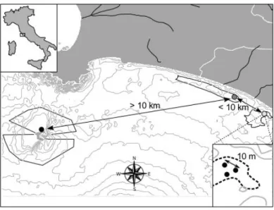
Organisms were collected in P. oceanica meadows from three sampling localities of the central Tyrrhenian Sea: two located along the mainland coastal area of Montalto di Castro (Chiarone and Punta Morelle) and one located in the insular area of Giannutri Island (Fig. 3.1).

Figure 3.1 - Overview of the study area. Black, light and dark grey circles are for Giannutri Island (GIAN), Chiarone (CHIA) and Punta Morelle (MOR), respectively. Arrows show the approximate distances between sampling sites at macro (> 10 km) and meso-scale (< 10 km). Insert at the bottom left shows a sketch of the sampling strategy at micro-scale (~ 10 m).

Chiarone (CHIA) is a Special Area of Conservation (Habitats Directive 92/43/EEC, SAC IT6000001) bounded by the estuaries of Chiarone River (to the North) and Fiora River (to the South). Depths range between 5 and 30 m, with an average of 18 m and a

prevalence of sandy-muddy bottoms due to the alteration of the sedimentary regime. Punta Morelle (MOR) is a Special Area of Conservation (Habitats Directive 92/43/EEC, SAC IT6000002) with an average depth of 25 m, ranging from 10-30 m. Seabed consists mainly of sandy substrate with rocky outcrops up to about 300 m from the shore, with a diversified morphology characterized by pools and jagged bathymetric. Giannutri Island (GIAN) is part of the National Park of Tuscan Archipelago. It is a limestone island characterized by a rugged and rocky coastline, where P. oceanica meadows are confined to the coastal areas due to the steep slope of the rocky seabed and the scarcity of shallow water bays.

Localities were further characterized on the basis of specific environmental characteristics known to be related with the boundaries of a variety of marine species, whose distribution at regional to local-scale are often limited by factors such as salinity, nutrient supply, topographic complexity and sediments (Briggs, 1995; Sbrocco and Barber, 2013). In particular, the persistence of amphipod communities is thought to be related to a series of complex mechanisms, including indirect effects of anthropogenic impacts on the meadows. The degree of water transparency, for instance, is an important parameter in regulating the importance of P. oceanica in the carbon budget of littoral Mediterranean ecosystems, as its depth limit is closely linked to light penetration underwater (see review in Duarte, 1991). Moreover, seagrass meadows produce excess of organic carbon over community requirements (Gattuso et al., 1998), which are believed to store an important fraction of the excess carbon they produce in the sediments (Duarte and Cebrián, 1996). Besides internal production, the deposition of organic matter can also be associated to a significant input of external nutrients, which develops communities with particularly high biomass (Duarte and Chiscano, 1999) and

slow decomposition rates (Romero et al., 1992; Mateo and Romero, 1997), thus influencing the composition of invertebrate communities.

Localities were therefore characterized by means of four key environmental parameters, namely: i) salinity, ii) sea surface temperature, iii) chl-a concentration and iv) water transparency measured by the diffuse attenuation coefficient at 490nm (kd490). Data

about salinity and temperature were downloaded as 1 km (30 arc-second) grid from MARSPEC (www.marspec.org), a high-resolution global marine dataset that combines variables from the benthic and pelagic environments into a single database (Sbrocco and Barber, 2013). Temperature and salinity were downloaded as raw monthly climatological layers for the reference season. Chl-a concentration and kd490 were

downloaded from AquaMODIS (http://oceancolor.gsfc.nasa.gov/cms/) as seasonal climatology (reference period 2002-2014) as 4 km resolution raster, downscaled throughout the contiguous study extent to the MARSPEC 1 km grid system using bilinear interpolation.

Spatial data are however characterized by specific properties, such as heterogeneity and autocorrelation, which can make them difficult to visualize and interpret. Heterogeneity means that processes can vary locally and are not necessarily the same at each spatial location, while spatial autocorrelation means a certain degree of relationship between variables at some location. Spatial heterogeneity and autocorrelation may sometimes invalidate two basic assumptions of many standard statistical analyses, that is, data independence and distribution. Moreover, spatial data may sometimes be highly dimensional (i.e. high number of variables measure at each observation) and thus difficult or redundant to visualize and interpret. However, a small amount of intrinsic dimensionality in the data sets may exists so that not all variables are needed to

understand specific processes of interest. Therefore, one solution is to reduce the dimensionality of the data to capture the maximum information present in original data and remove spurious or redundant data, minimizing the error between the original data and the new lower dimensional representation (Fodor, 2002).

Environmental parameters were therefore subjected to a Principal Component Analysis (PCA), to identify combinations of variables that best explain the variance in the data, reducing dimensionality and defining suites of variables that may be functionally related. As PCA assumes normality in the distribution of data, it is sensitive to the relative scaling of the original variables and, when these assumptions are violated, the resulting principal components may not be independent. Therefore, variables were centered to 0 and scaled by their variance using a z-score transformation. Localities were finally characterized by averaging the scores of the first axis of the PCA within the arbitrary boundaries given by the extent of protected areas. Spatial statistic analyses were performed with SAGA-GIS (SAGA Development Team, 2008).

3.2 Sampling methods

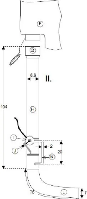
Sampling was carried out by SCUBA diving at the same depth range (15-20 m), as depth gradient and correlated factors are thought to play a crucial role in defining amphipod assemblages (Scipione et al., 1983; Mazzella et al., 1989). An air-lift sampler (500 µm mesh size), originally described in Bussers et al. (1983), was used in a 40 x 40 cm quadrant subjecting each sample to suction during two minutes of constant air flow (Fig. 3.2).

Figure 3.2 - Air-lift sampler (500µm mesh size), originally described in Bussers et al. (1983).

Samples were sieved on a 500 µm mesh and fixed in a 70% ethanol solution as soon as possible and then sorted out under a dissecting microscope. Amphipods were separated, identified to the species level and then counted. The identification was carried out using the taxonomic key of Ruffo (1982), with taxa nomenclature following the World Register of Marine Species (WoRMS, 2015; http://www.marinespecies.org).

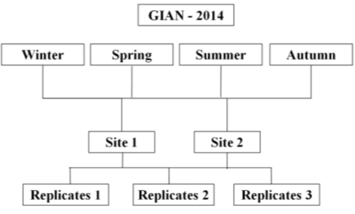
To investigate the spatial variation and structuring mechanisms of amphipod communities over the years, three sampling sites for each three localities (CHIA, MOR, GIAN) were considered in August 2012 and 2013 (Fig. 3.3). To evaluate instead the seasonal fluctuations, samples were collected only in the area of Giannutri Island during 2014, in the months of February, May, August and November, taking three random samples for each season in the two sites of Punta Secca and Secca di Punta Secca (Fig. 3.4).

Figure 3.3 – Sampling design for the spatio-temporal analyses of amphipod assemblages from Posidonia oceanica.

Figure 3.4 – Sampling design for the seasonal analyses of amphipod assemblages from Posidonia oceanica in Giannutri Island (GIAN).

To understand how the assemblages of amphipods varied in space and time, three level of spatial scales were considered to analyze the metacommunity structure: micro-, meso- and macroscale. Microscale analysis consists in describing the patterns within each locality (CHIA, GIAN, MOR). At mesoscale level, patterns of metacommunity were described considering the two coastal localities of Montalto area (CHIA vs. MOR) while, finally, the macroscale analysis involved also the area of Giannutri (GIAN vs. CHIA vs. MOR).

3.3 Statistical analyses

3.3.1 Spatio-temporal analysis

Data resulting from the taxonomic analysis of seasonal and annual samples were arranged as sites x species matrices, and specific community parameters, total abundance (n), species richness (S), Shannon-Wiener diversity index (H’) and Pielou’s evenness (J) were measured.

A diversity t-test based on bootstrap randomization with 1,000 replicates was used to test for seasonal differences among sites in GIAN. Mean values (± SD) of indices were measured for each locality (CHIA, MOR, GIAN) and differences with respect to factors localities (L, fixed factor with three levels corresponding to each locality) and years (Y, fixed and orthogonal to L, with two levels corresponding to different summer seasons) were measured by means of a two-way ANOVA. Prior to analysis, homogeneity of variances was checked using Levene’s test and transformations were applied when necessary.

The structure of amphipod assemblages was compared by a two-way permutational multivariate analysis of variance (PERMANOVA, Anderson, 2001), considering the factor Time (four and two levels fixed for the seasonal and annual comparison, respectively) and Localities (three levels fixed and orthogonal) with 9,999 permutations. A non-metric multidimensional scaling analysis (nMDS) was performed to display similarities in amphipod assemblages, and the Kruskal stress value tested the goodness of fit in the nMDS ordination diagram. A stress value < 0.2 is considered to provide a useful ordination. Analyses were based on the Bray-Curtis similarity matrices calculated

from the square root transformation of abundance data to overcome the contribution of rare species. A similarity percentage analysis (SIMPER) was used to identify those species that most influence the dynamics and the structure of communities.

Statistical analyses were performed with PRIMER v6 (Clarke and Gorley, 2006) and PAST 2.17 (Bing et al., 2013).

3.3.2 Pattern analysis

3.3.2.1 Commonness and rarity in community structure

For each scale of analysis, data were arranged as incidence matrices, which describe the presence of a given species (row) in a given site (column) (Presley and Willig, 2010; Silva et al., 2013). Most of marine communities have highly asymmetric distribution, with few abundant species and many rare species that frequently carry relevant information about the structuring of communities, as they may represent a relevant percentage of the total. The percentage of rare species at different scales of investigation was therefore quantified using the inflection point criterion on the rank-abundance curve, that is, the region of the curve at which the curvature changed (Siqueira et al., 2012). A piecewise regression on the raw abundance data was used to stress the real differences between common and rare species (Magurran, 2004), and comparing the goodness of fit of the piecewise regressions with the equivalent linear regressions by ANOVA.

3.3.2.2 Elements of Metacommunity Structure

To determine the pattern of best fit for amphipods distributions at different spatial scales, was used the Elements of Metacommunity Structure (EMS) approach by investigating coherence, species turnover and boundary clumping (Leibold and Mikkelson, 2002; Presley and Willig, 2010). The first step in EMS is to create an ordination of sites and species with respect to specific gradients or by means of ordination techniques able to uncover latent environmental gradients, so that different techniques and types of data (i.e. quantitative vs. qualitative) lead to different results in the analysis of the observed patterns. For this reason, quantitative data should be used only if there are reliable estimates of abundances for each species for each site. Sampling in natural conditions is by definition subjected to errors, especially in marine environment where biases are often related with the strongly asymmetric trends in patterns of species abundance.

Sites by species incidence matrices were ordered via reciprocal averaging technique, also known as correspondence analysis, which re-order rows and columns using repeated averaging of species and sites scores and maximizing their correspondence (Leibold and Mikkelson, 2002; Presley and Willig, 2010). Reciprocal averaging allows to reach a compromise between minimizing the number of range interruptions and the number of gaps in the community compositions of sites (Leibold and Mikkelson, 2002; Presley et al., 2009) and to detect variation in species distributions subjected to latent processes such as environmental gradients or variation in unmeasured environmental variables (Gauch et al., 1977). The primary axis represents the best possible ordering of sites and species to maximize their correlation, although in reciprocal averaging multiple ecologically meaningful ordinations may be possible, with each ordination axis

capable of representing a distinct pattern of species distributions along distinct gradients (Presley et al., 2009). In reciprocal averaging, the percent inertia (i.e. the degree of correlation between sites and species achieved by the ordination) of the primary axis could be relatively low with respect to the second axis (Gauch, 1982). Therefore, to evaluate the relative correspondence achieved by the ordinations on each axis, inertia values should be compared with those from different axes to understand whether or not more than one dimension may provide insights into EMS.

To test for a statistical significance in metacommunity patterns, a series of different, scale-dependent null-models were employed to resemble the incidences in the sites by species matrices, as different scales should constraints the distribution of species in different ways. Null-models in ecology are known to be affected by different statistical pitfalls, often related with types of models employed, spanning from extremely liberal (highly prone to type I errors, Gotelli, 2000) to extremely conservative (highly prone to type II errors, Gotelli, 2000). However, while trying to minimize the statistical errors associated with them, the appropriate choice of a null-model should be context-dependent, having in mind the biology of the system under study (Presley et al., 2009).

Amphipods are known to have low active dispersal ability due to the lack of pelagic larval forms (Thomas, 1993), also showing a wide range of responses to habitat modification (Vázquez-Luis et al., 2009), spanning from high specificity to tolerance towards alteration resulting from pollution, invasion by alien species and other disturbances (Guerra-García and Garcìa-Gòmez, 2001). Therefore, at different spatial scales, spanning from few tens of meters (micro-scale) up to tens of kilometers (macro-scale), the geographic isolation (insularization) of the meadows and the abiotic conditions should exert different roles in structuring communities. At micro-scale

(average distance ca. 10 m), no apparent effect of distance and abiotic conditions should influence the pattern of species distribution (Table 3.1) and, therefore, a null-model in which the total number of occurrences (fill) are fixed and all sites and species are equiprobable (Gotelli, 2000) was used. At meso-scale (average distance <10 km), the distance between localities increases its importance in the structuring of communities, although similar abiotic conditions (Table 3.1) and, therefore, was used a null-model that only maintains species frequencies (Jonsson, 2001). Finally, as the macro-scale involves high distances between localities and different abiotic conditions, species distribution should depends on their frequencies of occurrence and abiotic tolerance (Table 3.1). Therefore, a null-model with fixed rows (diversity of sites) and column marginal frequencies as probabilities of selecting species was employed.

A final remark should be done with respect to the dimension (i.e. number of rows x columns) of the matrices, which may influence the statistical significance of the randomization procedures. To avoid specific statistical pitfalls, we used a number of randomization in the EMS algorithm proportional to the maximum number of possible substitutions in a matrix, and iterated n times the micro-scale analysis until a stable solution was reached. Although such a statistical artifice can somehow reduce the degree of uncertainty in the interpretation of results, these should however be taken with caution.

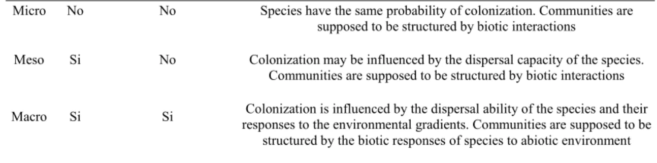
Table 3.1 - Hypothesized effects of space and environment on the distribution of amphipods in Posidonia oceanica meadows at different spatial scales.

Scale Space Abiotic environment Rationale

Micro No No Species have the same probability of colonization. Communities are supposed to be structured by biotic interactions

Meso Si No Colonization may be influenced by the dispersal capacity of the species. Communities are supposed to be structured by biotic interactions Macro Si Si _{responses to the environmental gradients. Communities are supposed to be}Colonization is influenced by the dispersal ability of the species and their

structured by the biotic responses of species to abiotic environment

Coherence was evaluated by counting the number of embedded absences in a matrix ordered according to the primary axis. Significant negative coherence results if the number of embedded absences randomly obtained is lower than the observed number of embedded absences, and indicates that species presences follows a checkerboard pattern. A non significant coherence means that the metacommunity is randomly structured whereas a significant positive coherence suggests that species are distributed according to the same gradient (Leibold and Mikkelson, 2002; Silva et al., 2013). When positively coherent, the EMS analysis continues evaluating species turnover and boundary clumping, to compare the distribution of species among sites. Turnover was measured as the number of times one species was replaced by another species between two sites. If the turnover is significantly low, the metacommunity shows a nested distribution, conversely, if the metacommunity exhibits a non significant or a significant positive turnover, it is consistent with the remaining distribution patterns. Finally, the boundary clumping was evaluated with Morisita’s index (Morisita, 1971), to distinguish among evenly spaced, Gleasonian and Clementsian distributions (Leibold and Mikkelson, 2002; Silva et al., 2013).

4.

RESULTS AND DISCUSSION

4.1 Seasonal fluctuations in amphipod communities associated with

Posidonia oceanica meadows of Giannutri Island

4.1.1 Results

Samples were collected at Giannutri Island in 2014 during four seasonal sessions, providing a total of 1,144 individuals belonging to 62 species and 24 families. The most abundant species were Apherusa chiereghinii (110 individuals), Liljeborgia dellavallei (105 individuals), Apolochus neapolitanus (91 individuals), A. picadurus (73 individuals), Gitana sarsi (66 individuals). Some species were present in every season at varying abundances, such as Dexamine spinosa (63 individuals overall), and Synchelidium longidigitatum (35 individuals overall). Other species were recovered in single seasons: Caprella acanthifera appeared only in springtime while Maera grossimana, M. hamigera and Gammarella fucicola were present only in autumn, this latter at appreciable abundance (42 individuals).

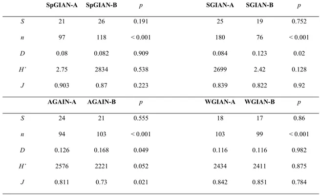
The comparison between the two sampling points (Punta Secca-A and Secca di Punta Secca-B) showed substantial homogeneity, since only the number of individuals (n) significantly varied (Table 4.1) between sites in each season (bootstrap diversity t-test, p < 0.001 in all cases). Differences were observed for other parameters without a seasonal pattern, therefore suggesting that no real differences exist: dominance (D) in summer (bootstrap diversity t-test, p = 0.012), Shannon diversity (H’) and evenness (J) in autumn (bootstrap diversity t-test, p = 0.040 and p = 0.021, respectively). The number

of taxa (S) did not show any significant difference between sites in all seasons (bootstrap diversity t-test, p > 0.05).

Table 4.1 - Comparison of seasonal pattern of diversity between localities: S = number of species; n = total number of individuals; D = dominance; H’ = Shannon’s diversity index; J = Pielou’s evenness index.

Sp = Spring; S = Summer; A = Autumn; W = Winter. A is for Punta Secca, B is for Secca di Punta Secca

A two-way PERMANOVA was carried out to test for the factors that mainly affected the structural differences in community composition, showing the significant influence of ‘seasonality’ (F = 3.019, p < 0.001) and no influence of the factor ‘space’ (F = 1.333, p > 0.06). The nMDS ordination plots evidenced highest variability in specific seasons and less pronounced differences in others, with a partial overlap of Winter, Spring and Summer, in contrast with a clear separation of the Autumn (Fig. 4.1, Kruskal stress = 0.18).

SpGIAN-A SpGIAN-B p SGIAN-A SGIAN-B p

S 21 26 0.191 25 19 0.752

n 97 118 < 0.001 180 76 < 0.001 D 0.08 0.082 0.909 0.084 0.123 0.02

H’ 2.75 2834 0.538 2699 2.42 0.128

J 0.903 0.87 0.223 0.839 0.822 0.92

AGAIN-A AGAIN-B p WGIAN-A WGIAN-B p

S 24 21 0.555 18 17 0.86

n 94 103 < 0.001 103 99 < 0.001 D 0.126 0.168 0.049 0.116 0.116 0.982

H’ 2576 2221 0.052 2434 2411 0.875

Since the two sampling points showed to be substantially homogeneous, data were cumulated per season and analyzed comparing the diversity indices, in order to highlight the fluctuations of the community throughout the course of the year.

Figure 4.1 - nMDS ordination plot of the sampling sites in different seasons.

The number of recovered taxa and the Shannon diversity index increased from winter ahead during the year, reaching their maximum peak in autumn (Table 4.2).

Table 4.2 - Seasonal trend of the biodiversity components. S = number of species; n = total number of individuals; D = dominance; H’ = Shannon’s diversity index; J = Pielou’s evenness index. Sp = Spring; S = Summer; A = Autumn; W = Winter.

Sp S A W S 31 31 34 24 n 215 256 197 202 D 0.072 0.083 0.106 0.107 H’ 2.966 2.781 2.722 2.545 J 0.864 0.81 0.772 0.801