2015
Publication Year
2020-03-30T14:37:27Z
Acceptance in OA@INAF
Analysis of the kinematics of ejecta created after a catastrophic collision
Title
DELL'ORO, Aldo; CELLINO, Alberto; Paolicchi, P.; Tanga, P.
Authors
10.1016/j.pss.2015.09.009
DOI
http://hdl.handle.net/20.500.12386/23707
Handle
PLANETARY AND SPACE SCIENCE
Journal
118
Analysis of the kinematics of ejecta created after a
catastrophic collision
A. Dell’Oroa,∗, A. Cellinob, P. Paolicchic, P. Tangad
aINAF - Osservatorio Astrofisico di Arcetri, Largo E. Fermi 5, 50125 Firenze, Italy bINAF - Osservatorio Astrofisico di Torino, Strada Osservatorio 20, 10025 Pino
Torinese, Italy
cUniversit`a di Pisa, Dipartimento di Fisica, Largo Pontecorvo 3, 56127 Pisa, Italy dObservatoire de la Cˆote d’Azur, Bv de l’Observatoire - CS 34229, 06304 Nice Cedex 4,
France
Abstract
According to the results of hydrodynamical simulations, the creation of an asteroid dynamical family as the outcome of a high-energy collision con-sists of the partial or complete shattering of the parent body followed by re-accumulation of many fragments into larger bodies due to the mutual gravity. This scenario seems to reproduce satisfactorily the observed properties of the asteroid families, and in particular the size distribution of the members. In this paper we show a preliminary analysis of the ejection velocity fields pre-dicted by hydrodynamical models, in comparison with the ejection velocity fields simulated by semi-empirical models, in order to identify the features of the velocity distribution that trigger or prevent the fragments’ gravitational re-accumulation.
Keywords: Asteroids, impacts, fragmentation, SPH models,
∗Corresponding author
Email addresses: [email protected] (A. Dell’Oro), [email protected] (A. Cellino), [email protected] (P. Paolicchi), [email protected] (P. Tanga)
Semi-Empirical Models
1. Introduction
According to current understanding (see, for instance, Michel et al., 2015, and references therein) the creation of a dynamical family of asteroids as the outcome of a high-energy collision event can be schematically described as a three-step process: (1) a hydrodynamical phase, in which the colliding system (projectile+target) is partially or completely shattered and fragments are cre-ated and ejected from their original locations; (2) a ballistic phase, in which the ejecta may experience mutual collisions and/or may be re-accumulated under the effect of gravitational interactions; (3) a dynamical phase in which each fragment is an independent body orbiting along a separate trajectory around the Sun, subject to gravitational and non-gravitational perturbations present in the Solar System. At the end of the phase (2) the final physical structure of the asteroid family is established, and its observable properties, also after a long dynamical evolution, can keep significant footprints of the original event from which it was originated. The size distribution of the members of the family is closely connected to the physics of fragmentation of the parent body and ejection of the fragments (the latter process possibly in-cluding collisions and re-accumulation). The overall structure of a dynamical family observed after its formation is a consequence of the initial distribution of fragment ejection velocities, (and their possible correlations with the frag-ment sizes), and the subsequent evolution due to gravitational perturbations by the planets and non-gravitational forces (Bottke et al., 2001; Carruba et al., 2003; Cellino et al., 2004; Vokrouhlick´y et al., 2006). More recently,
the additional role of non-destructive collisions among asteroids producing a weak, but stable transfer of linear momentum has also been outlined by Dell’Oro & Cellino (2007); Wiegert (2015).
In this paper we focus on the phases (1) and (2) described above. A lot of work has been done in the past to investigate the physics of inter-asteroid impacts and the predicted outcomes in terms of size distribution, ejection ve-locities, spin rates and shapes of the fragments. The final goal of such studies is to correctly understand and interpret the observable properties of aster-oid families, considered to be the outcomes of catastrophic collisions. The problem has been addressed in laboratory experiments (impacts involving centimeter-scale targets) as well as by means of theoretical models. In turn, different theoretical approaches have been followed. Numerical models based on fundamental laws of the hydrodynamics (known as Smoothed-particle hy-drodynamics (SPH) models, or briefly hydrocodes) have been developed and proved to work to reproduce the outcomes of laboratory experiments (Melosh et al., 1992). Attempts to extend the models to the case of impacts among asteroids have been done (Love & Ahrens, 1996; Ryan & Melosh, 1998). Us-ing hydrocode models, Benz & Asphaug (1999) computed the impact energy threshold for fragmentation characterizing typical impacts between Main Belt asteroids, a result that has been independently confirmed by models of col-lisional evolution of the whole asteroid population (Bottke et al., 2005).
Hydrocode models usually succeed in reproducing well the size distribu-tions of fragments produced in impact experiments in laboratory. When ap-plied to simulate collisions among kilometer-size bodies in the asteroid Main Belt, however, hydrocodes predict a complete fragmentation of the parent
body down to sizes corresponding to the numerical resolution of the model (Benz & Asphaug, 1999). Such complete “pulverization” of the parent body is in contrast with the observational evidence about the size distributions of asteroid families members, which tend to follow a power law size distribution. In most cases the sizes of fragments predicted by hydrocode models would be much smaller, to the point that family members would be too faint to be detected, ruling out even the mere possibility to identify families.
The discrepancy between hydrocode outcomes and the observed size dis-tributions of asteroid families has been solved by suggesting that family members have sizes that are eventually produced by a process of massive gravitational re-accumulation occurring at the end of the ballistic phase (2). This scenario has been demonstrated by Michel et al. (2001), who made a numerical simulation of the formation of the Eunomia and Koronis asteroid families. In practical terms, Michel et al. (2001) used the output of hydrocode models as the input of a N-body integrator in order to follow the dynam-ical evolution of the system of particles and detect their mutual collisions for several days after fragmentation. The results of Benz & Asphaug (1999) already suggested that at least the family largest remnant could be the result of a gravitational re-accumulation of fragments, forming a so-called rubble-pile, but Michel et al. (2001) showed that many smaller family members can also be the product of a re-accumulation, too. A perfect match between the observed size distributions of the major families and those predicted by this model has never been obtained, because the observed size distributions tend to be shallower than the predictions; however, this can be explained as the result of subsequent collisional evolution of the families (Michel et al., 2002).
The key result is: it is possible to obtain an “ordered” re-accumulation char-acterized by a power law distribution of the final family members, starting from the ejection velocity field provided by hydrocodes.
An approach similar to that of Michel et al. (2001) had been tried before by Pisani et al. (1999). These authors did not use the outcomes of hydrocode models, but assumed as initial condition of the ballistic phase (2) the ejection velocity fields predicted by some Semi-Empirical Models (SEM) developed in the 90’s (Paolicchi et al., 1989, 1996). The SEM was originally developed to closely mimic the observed kinematic properties of fragments produced in laboratory experiments of catastrophic breakup events. In the most recent versions of SEM, a more accurate treatment of the evolution of fragments during the ballistic phase has been included, incorporating an N-body inte-gration to follow the dynamical evolution of the fragments (Paolicchi et al., 1996; Doressoundiram et al., 1997). In Pisani et al. (1999) the model param-eters of the SEM were tuned in order to obtain a good match between some distributions of initial ejection velocities predicted by the hydrocode model of Love & Ahrens (1996) and those predicted by the SEM. At that time hydrocodes were able to compute only the size and velocity distributions of the fragments, but not yet a detailed list of initial positions and velocities for individual fragments. Pisani et al. (1999) did not assign to the fragments the sizes predicted by the SEM on the basis of some considerations based on the properties of the ejection velocity field (Paolicchi et al., 1989, 1996), but they divided the parent body into a number of small and equal spheri-cal particles, to match more closely the hydrocode outcomes. This analysis, however, failed to reproduce the observed size distributions of asteroid
fam-ilies. The results suggested that the re-accumulation involves only one or very few fragments (the largest remnant and a few other bodies), and the observed size distributions of asteroid families could not be reproduced.
This lack of re-accumulation processes during the ballistic phase of family formation as modelled by the SEM is somehow puzzling, taking into account that this model closely reproduces the kinematic properties of the fragments produced in laboratory experiments. One could object that the gravitation is negligible in the experiments, whereas it can be much more important when much larger bodies are involved in catastrophic collisions. On the other hand, it is not easy in any case to obtain a significant re-accumulation into many, larger bodies, from a set of small fragments moving outwards as the effect of an ejection velocity field (for example in simple kinematic models as a purely spherical expansion). It is therefore natural to wonder whether some special properties of an ejection velocity field are necessary to trigger a general process of re-accumulation in agreement with both the results of hydrodynamical codes by Michel et al. (2001), and with the existence of observable asteroid families.
To try and find an answer to this question, we have analyzed in depth two velocity fields produced by the SPH model used by Michel et al. (2001) and used them as the input of an N-body integrator in order to simulate the ballistic phase of the two simulated events. Having at disposal for the moment only two examples of SPH ejection fields, in this paper we can show only some partial results, and we plan a more extensive analysis in the future. We name the two fields “50k” and “koronis”. The field “50k”, obtained by the fragmentation of a parent body about 200 km in size, produced a
fast re-accumulation into a largest remnant and many smaller bodies. The field “koronis” has been produced by Michel et al. (2001) to fit the observed properties of the Koronis family, characterized by a relative small largest remnant. This field was produced by assuming a much larger impact energy than in the case of the “50k” and a parent body having a diameter of 119 km, corresponding to the estimated size of the parent body of the Koronis family.
The aim of the present work is to compare the final outcomes of these two SPH ejection velocity fields and those predicted by the SEM starting from the same sets of initial conditions, in order to shed light on the quali-tative differences that make the final outcomes of those models so different. We note that this investigation is not only interesting per se, but it can have implications also for what concerns investigations aimed at assessing the pos-sible formation of binary systems in family-forming events (Doressoundiram et al., 1997).
2. Direct collisions among fragments
The approach we follow in this work is not simply to carry out again an N-body numerical integration starting from the initial conditions of the particles after the hydrodynamical phase, to analyze the final outcome of the ballistic phase. What we do is rather to investigate directly the geometrical and kinematic properties of the system of particles at the beginning of the ballistic phase, namely the properties of the initial ejection velocity field before any evolution.
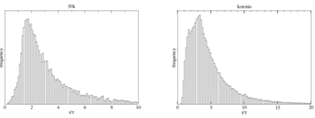
Figure 1: Distribution of the epoch of collision for the pair of fragments involved in direct impact. The epoch zero is the initial epoch of the ballistic phase. The characteristic time τ is the time the system takes to double its size.
“koronis” may occur even if no mutual gravitational attraction is taken into account. In other words, if we assume that each fragment is moving along a straight line with a constant velocity, supposed to be simply equal to the initial ejection velocity (this assumption is equivalent to switch off the effects of gravitation), we can easily compute the epoch of closest approach and the corresponding minimum distance between the members of all possible couples of fragments. If this minimum distance is less than the sum of the radii of the two bodies, a collision must take place, and this is exactly what we found in many cases. In other words, among fragments of the SPH models under investigation, some pairs of fragments follow initial trajectories which are convergent.
In particular, the test field “50k” is composed by 42, 403 particles. Among them, 11, 696, corresponding to 28% of the total mass are found to have convergent initial trajectories. In the case of the “koronis” model, 43, 804
particles out of a total number of 212, 100 have convergent trajectories (21 % of the total mass). We can use, as a time unit for the evolution of the system, the characteristic time τ needed to make the system twice as large compared to its initial size. In turn, the size of the system is defined as the average of the mutual distances of all the ejected particles. As shown in Fig 1, in the case of “50k”, 80% of direct impacts occur before 4τ -5τ , with a peak around 2τ , while for “koronis” the majority of impacts occurs before 7τ , with a peak around 3τ -4τ .
It is interesting to note that the characteristic time τ turns out to be about 3.5×10²s for “50k” and 1.8×10² s for koronis, much shorter compared to the dynamical time of the system 1/√Gρ (where ρ is the density), of the order of 2 × 10³ s. This means that direct collisions occur over a time scale much smaller than the dynamical time, or in other words when the initial rectilinear trajectories are still unaffected by the mutual gravitational attraction among the particles. To investigate how direct collisions affect the trajectories of the particles, looking for second-generation collisions, is not necessary for the scopes of the present work, where we want to outline the existence of direct collisions without the intervention of the gravity as the symptom of peculiar properties of the structure of the ejection velocity field. The number of collisions we have reported above is a lower limit of all possible collisions. On the other hand the rate of collisions decreases very quickly as the system expands, and so we reasonably expect that the contribution of the second-generation collisions should be very low.
The bare existence of this effect marks a significant difference with SEM models. In SEM the ejection velocities of the fragments are assigned
as-suming the existence of a continuous ejection velocity field throughout the fracturing body (Paolicchi et al., 1989). In the absence of a rotation term due to the original spin of the parent body and to a possible transfer of an-gular momentum by the projectile, the assumed velocity field has two basic characteristics:
1. the velocity vector associated to each point of the parent body is ori-ented along a straight line originating from a single point of irradiation (IP) which is common to all fragments;
2. the module of the velocity field vector increases monotonically moving away from the irradiation point.
The effect of angular momentum can be computed by adding to the ejection velocity field vector an additional term corresponding to a rigid rotation around a given spin axis. Based on the above properties, SEM models do not allow for the possible existence of convergent initial trajectories involving any couple of fragments (i, j). In fact, the purely radial ejection component of the field produces all divergent trajectories, and the additional term due to rotation has the form ~ω × (ri− rj), where ri and rj are the initial position
of two particles with respect to the center of the target, and thus cannot decrease the distance between any couple of fragments.
3. Investigating the geometric structure of the ejection fields
Our main goal is to identify the properties of SPH velocity fields that make it possible for them to allow for the presence of fragments on convergent trajectories, something that is not possible under the assumptions of the
SEM. As we have already mentioned, the existence of one single irradiation point is a major assumption of the SEM. Direct collisions are not allowed if one IP exists and the velocities are monotonically increasing with the distance from it. As a consequence, it seems that the ejection velocity fields produced by the SPH cannot either have irradiation points, or monotonically increasing velocities from it, or neither of them.
Since this seems to be a critically important point, we will now define a generalized concept of irradiation point, the irradiation point in the SEM being only a particular case of it.
3.1. Trajectories’ focusing analysis
Let us have a system of N particles, each characterized by a mass mj and
a diameter dj (we assume, for sake of simplicity, that they have spherical
shapes). The position and velocity of each particle are given by the rj and
vj vectors, and the positions are defined with respect to a given reference
system. Hereinafter the symbol rj will mean the position of the j-th particle
at the epoch t = 0, while rj(t), is the position at an arbitrary epoch t. In
the analysis of the velocity field, we will always assume that the vectors vj
are constant, while obviously rj(t) = vjt + rj. From a physical point of
view, epoch t = 0 corresponds to the end of the fragmentation phase and the beginning of the ballistic phase.
In the SEM the irradiation point is the only one point which is crossed by the trajectories of all fragments, if we neglect any term due to rotation. In particular, each trajectory can be described by a line passing through the location described by the vector rj, and parallel to the vj velocity vector.
This condition can be formally written as vj = f (rj)(rj− r∗), where f (r) is a
scalar function of the position, and r∗ is the position of the IP. Such relation
is assumed to hold only at t = 0. If the module of the velocity is assumed to be simply proportional to the distance from the IP (that is, if f is a positive scalar constant k), at a given time t = −1/k < 0 all particles would overlap with the IP. If the velocities are not simply proportional to the distance from IP, such virtual event does not take place, because each fragment would pass by the IP at a different time. 1
It is important to note that the assumed properties of the SEM ejection velocity field do not guarantee that the barycenter of the system is at rest: the reason is that the SEM velocity field is defined in the reference system of the IP, not in the reference system of the center of mass. The choice of the reference system obviously determines the properties of the velocity field: passing from a reference frame to another, the velocity of the j-th fragment becomes v0j = vj + w, where w is a vector common to all fragments, and
thus the field will be now described by the relation: vj0 = f (rj)(rj− r∗) + w
The question is now the following: Does it exist a (fixed) point r0∗ such that:
vj0 = f0(rj)(rj− r0∗)
where f0 is a suitable scalar function of the position?
1Actually, what happens is that SEM assumes that before t = 0 there is no motion, and
one can assume that all the fragments are still located in their original locations rj within
the parent body. It is true, however, that the assumption that all fragments achieve their ejection velocity vj exactly at the same time t = 0, is not realistic.
If f is a constant scalar k, r0∗ = r∗ − w/k, and again f0 = k. This is a
remarkable and well known property of linear fields: for instance, it is the same reason why in a universe expanding according to a Hubble law it is pos-sible to define every point as the virtual center of expansion (“cosmological principle”)
However, apart from such special cases, in general the IP no longer exists for any f (rj) if we change the reference system. The answer to our previous
question, is therefore, generally, no.
The SPH velocity fields under investigation are given in the reference system of the center of mass (CM). If we had to write a SEM velocity field in the CM system, we would be in trouble, because the existence of an IP should not be possible in general. From a geometrical point of view, if a velocity field is defined having an IP in a given reference system, a change of reference system will produce a sort of de-focusing of the trajectories of the particles. Thus, if we want to have an IP in a given velocity field, we have to choose a suitable reference system. The general question then becomes: does it exist a reference system in which the field has an IP?
In order to look for an IP we need a quantitative way to measure the degree of convergence, or focalization, of the trajectories in a given point O. A natural parameter is the minimum distance between the trajectory and the point. In the general case in which the point O is moving, the minimum distance si from the i-th trajectory is:
s2i = b2i − (ni· bi)
2
n2 i
= (bisin αi)2 (1)
the point O, respectively. The angle αi is the angle between the directions
of the relative velocity vi− v and of the relative position ri− r. If si = 0 for
all particles in the velocity field, than O is an IP of the field. For any generic point O, the parameter si has a particular distribution and we can define its
mean value: s2 = 1 N X i s2i (2)
as a measure of the degree of focalization of the particles’ trajectories with respect to the point O.
Now, we cannot expect that for any velocity field a point O must always necessarily exist, such that s2 = 0. Even if a velocity field was originally
characterized by the presence of an IP, it can well happen that the IP can be lost due to reasons not merely related to a change of the reference system. Rotational terms, for example, can overlap to the perfect velocity/position pattern and can modify the intrinsic geometric properties of the field. In particular, in the case of a SEM-like velocity field including a rotational term, it can be easily demonstrated that α 6= 0 and that s2/R2 is of the
order of the ratio Erot/Ekin, where R is the size of the body, and Erot and
Ekin are, respectively, the total energies due to the rotational motion and to
the ejection field 2 .
2In the SEM the velocity v is related to position by:
v = f (r)b + ~ω × r
where r is the position respect to the center of the parent body, and b = r − r∗. Being
|v × b|2= v2b2sin2α, it follows that s2v2= |v × b|2= |(~ω × r) × r
On the other hand, a certain degree of focalization of the particles’ tra-jectories may be preserved, and this is related to the point O for which s2
is minimum. For this reason we define the maximum focalization point, or simply the focalization point “FP” as the point O that minimizes the value of s2. The minimum value of s2 is a measure of the degree of focalization (or
convergence of the trajectories) of the field.
The parameters si and s2 are suitable for the characterization of the
intrinsic structure of the field. In fact, they are invariant with respect to the choice of the reference system (ni and bi do not depend on the reference
system). Moreover, they are constant in time, that is, by substituting in (1) r and ri with respectively vt + r and vit + ri, the value of si does not
change. These properties do not imply of course that the FP is invariant for any change of reference system or time evolution. If FP has a position r (at t = 0) and a velocity v, and we change the reference system by adding to each velocity vector a common vector w, the FP in this new reference system has position (at t = 0) and velocity respectively r and v + w, but with the same value of s2. Similarly, if at t = 0 the FP has position and velocity r and
v, at a different epoch t 6= 0 the FP has a new position vt + r, but preserving the same value of s2.
3.2. Searching the focalization point
s2v2 = v2 rotr2∗sin
2β, where v
rot = (~ω × r) is the rotational component of the ejection
velocity and β the angle between vrot and r∗. Noting that v2 scales as the total kinetic
energy Ekin, vrot2 scales as the total rotational energy Erot and r∗ as the radius of the
body, it follows that s2/R2 is proportional to the ratio E
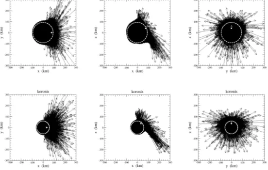
Figure 2: Velocity vectors (black arrows) for the field “50k” (top) and “koronis” (bottom). The white dot represent the position of the FP, while the white arrow its velocity. The circle drawn with a white dashed line shows the outline of the parent body.
From the mathematical point of view, the parameter s2 in (2) is a function
of the two vectors r and v, and it is therefore a property of the velocity field for which it is defined. By definition, the FP is the couple of vectors (r∗, v∗) that minimizes the value of s2. In principle, the search of the FP
is a problem of minimization of a function defined in the six-dimensional space of the position coordinates and velocity components. However, it is possible to reduce the problem to the minimization of a function defined in a three-dimensional space.
Let us consider for the moment the simpler problem of the minimization of the function s2(r, v) in the case v = 0. The vector r = (x, y, z) that
minimizes s2(r, 0) has to fulfill the following conditions:
∂ ∂xs 2(r, 0) = 0 ∂ ∂ys 2(r, 0) = 0 (3) ∂ ∂zs 2(r, 0) = 0
The conditions (3) are three linear equations of the unknown x, y and z, whose coefficients are functions of the positions ri and velocities vi of the
particles of the velocity field. Once such coefficients are computed, the solu-tion can be obtained by means of the inversion of a 3 × 3 matrix.
The point is that the minimum of the function s2(r, 0) can be computed
analytically in a direct (and fast) way. Then, if v 6= 0, and we look for the point r that minimizes the function s2(r, v) (keeping v fixed), it is always
possible to reduce to the case for which Eqs. (3) hold, by simply writing the velocity field in the reference system moving with a constant velocity v. This
means simply to add to each velocity vi the vector −v, and to invert the Eqs.
(3). In this way, for any value of v we can compute the point r∗ (depending
on v) that minimizes the function s2(r, v), assuming that v is fixed. We can
then compute the corresponding minimum value s2(r
∗, v). So now we have
just to find the value of v that minimizes s2(r
∗, v). The vectors r∗ and v∗
for which s2(r
∗, v∗) is the minimum value are the position and velocity of the
FP.
The last step cannot be done analytically and requires some kind of nu-merical approach. We implemented a strategy based on a genetic algorithm (Whitley, 1994; Schmitt, 2001). Being the search of the FP to be done only once for each of the two ejection velocity fields, we do not need high speed computing requirements. So we have chosen this approach because of its simplicity of implementation, despite of its slowness. In few words, a large set of triplets v = ( ˙x, ˙y, ˙z) is randomly generated, creating an initial popu-lation of reference systems. For each triplet, we compute the corresponding values of r∗ and s2(r∗, v). Then we evolve the population by creating new
triplets. A new triplet is created choosing randomly two different triplets already in the existing set and exchanging randomly the coordinates ˙x, ˙y, and ˙z of one triplet with the corresponding coordinates of the other triplet. Moreover small perturbations δ ˙x, δ ˙y, and δ ˙z are added to the components of the new triplet. At this point we identify the triplet already in the set with the largest value of s2(r
∗, v) = s2max, that is the “worst” triplet in the
population. If the new triplet is better than this worst triplet, that is if its value of s2(r
∗, v) is smaller than s2max, the worst triplet is removed from the
of times, to make the population of triplets to evolve, the values of s2(r ∗, v)
becoming increasingly smaller, and converging to the minimum value of the function s2(r, v).
We have tested this algorithm on simulated velocity fields having an IP and then writing positions and velocities in a different inertial reference sys-tem. In these cases the FP must be a perfect IP, that is the minimum of s2(r, v) is null. The velocity of the IP (that is the velocity of the reference
system in which the IP exists and is in rest) and its position were always successfully retrieved. In the special case that the velocity field was con-structed assuming the module of the velocity to be strictly proportional to the distance from the IP, the numerical method fails, because in any refer-ence system, that is for any v, the minimum of s2(r, v) is null, or in other
words an IP exists in all reference systems. But in this case the problem is solved by simply inverting the system of equations (3).
It is important to stress that it is not guaranteed that in general a fo-calization point exists for any velocity field. A trivial example is a field composed by only two particles with equal and parallel velocities. In this case the two trajectories do not intersect in any reference system, and the distance between the two trajectories can be reduced to zero only assuming v parallel to the line passing through the two particles and v → ∞. The same conclusion holds if we have many particles with equal and parallel ve-locities, for which probably the parameter s2 has a minimum but it does not correspond to a “focalization” of the trajectories that remain parallel. So, the convergence of the procedure described above cannot be guaranteed a priori, but it must be checked a posteriori, verifying the degree of radiality
of the trajectories respect to the obtained FP.
Using the above technique, we have obtained the FPs for the two SPH velocity fields under investigation. Fig. 2 shows the velocity fields at the beginning of the ballistic phase. The positions of the corresponding FP are represented with white dots. The value of the parameter s2 for the two
identified FP is 366 km2 and 136 km2, respectively for “50k” and “koronis”. Considering that the radius of the two parent bodies should be around 100 km and 50 km, the extensions of the convergence regions of the trajectory turn out to be about 20% of the size of the parent body. Apart from the degree of the convergence, in Fig. 2 velocity vectors appear to originate from a point that is well represented by the white dots. This is in reasonable agreement with the structure of the velocity field assumed by SEM based on the evidence coming from laboratory experiment. The difference is that in the cases simulated by SPH codes, the focalization of the trajectories is much less sharp than the SEM assumption. The rotational terms due to a non–central impact also contribute to increase s2 to a significant fraction of
the parent body’s cross-section. As discussed above, this tends to happen also in the case of SEM, when a spin term is added.
A significant feature of the FPs shown in Fig. 2 is that they are located very close to the surface of the parent body, at a distance from the center larger than 90% of the radius. This is different with respect to the usual SEM assumptions, but it might be consistent with the time–honoured assumption of “impact–explosion equivalence” and the related definition of the optimal burial depth (Melosh, 1989, p. 113).
v∗ is almost parallel to r∗, that is, the velocity of the FP is directed opposite
with respect to the center of the target, with an angle between the radial direction of about 20◦ in the case of “50k” and 15◦ for “koronis”. Moreover, the motion of the FP is directed towards the region of the parent body where the fastest fragments are ejected, that is, in general terms, toward the original impact point on the target’s surface.
We also note that the module of the FP velocity is found to be about 0.13 km/s for “50k” and 0.16 × 10⁴ km/s for “koronis”. Physically, the properties of v∗ should come out from the properties of the collision and from the choice
of the reference system in which the motion of the fragments is described. According to the Authors of the model, in the case of the “koronis” velocity field, the diameter of the parent body and the diameter of the projectile were assumed to be 119 km and 60 km, respectively, and the impact velocity of the projectile with respect to the target was assumed to be 3.25 km/s, with an incidence angle of 75◦ with respect to the normal to the surface at the impact point (Michel et al., 2001). It turns out therefore that the velocity of the FP is of the order of the linear momentum of the projectile divided by the mass of the target, and is therefore close to the normal component of the imparted linear momentum.
4. Geometrical properties of the fields
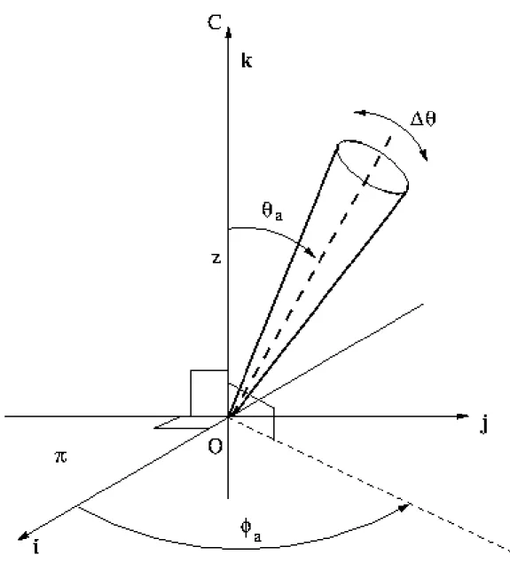
Figure 3: System of coordinates in the reference system at rest with the FP (origin “O”). See text for details.
The FP found for the velocity fields coming out from the ”50k” and ”ko-ronis” models are the SPH-equivalent of the IP assumed in SEM simulations. Thus it is reasonable to continue our analysis of the intrinsic differences be-tween SPH and SEM by studying the geometrical properties of the SPH field in a reference system in which the FP is at rest, in analogy with what hap-pens for SEM, where the breakup field velocities are given in an IP-centered reference system.
For a given particle, we will call ∆ri and ∆vi, respectively, the position
vector and the velocity vector of the i-th particle with respect to the FP: ∆ri = ri− r∗ and ∆vi = vi − v∗. We also introduce a system of cylindrical
coordinates having its origin O in the FP (Fig. 3). The vertical axis k is the line passing by O and the center C of the target, while the fundamental plane π is the plane normal with respect to the vertical axis and containing the origin O. On the fundamental plane a zero-azimuth axis i is defined. The choice of the axis i is arbitrary and it is needed only to define the azimuthal angle. For a given particle P , z is the distance of P from the plane π (positive if P belongs to the same semi–space containing C), while d is the distance between P and the axis k. If P0 is the projection of P on the plane π, the angle between the axis i and the line OP0 is the azimuthal angle φ, with the convention that φ = +90◦ for the vector j = k × i. The angle θ is the polar angle defined in the range [0◦, 180◦] between the axis k and ∆ri.
The parameters we have defined describe the spatial distribution of the particles around the FP. In general, the vectors ∆vi are not perfectly parallel
to the corresponding ∆ribeing the FP not exactly an IP. In order to quantify
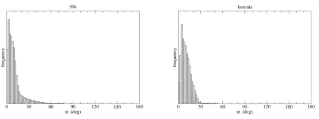
Figure 4: Distributions of the deviation angles α. The deviation angle is the angle α between the vector ∆r connecting the FP to the particle and the velocity vector ∆v of the particles with respect to the FP.
define a deviation angle α, namely the angle defined in the range [0◦, 180◦] between ∆vi and ∆ri.
All the plots in the next sections, showing the distributions of the above defined parameters, have been executed by propagating the positions of the particles and the position of the FP to the epoch when the size of the system is minimum, in order to get as close as possible to the moment in which the particles begin to separate from each other.
4.2. Analysis of the data
Fig. 4 shows the distributions of the deviation angle α. The typical deviation from perfect radiality with respect to the FP is of the order of 10◦-15◦, both for “50k” and “koronis”. The fact that the distributions of the angle α is not a Dirac delta function centered at zero is another way to show that for those velocity fields an ideal IP does not exist. This property is
clearly related to the existence of crossing trajectories which make it possible to have mutual collisions among the fragments.
The relevance of the rotational term produced by the angular momentum imparted by the projectile to the parent body as a cause of the misalignment of the velocities ∆vi with respect to the position vector ∆ri is not easy to
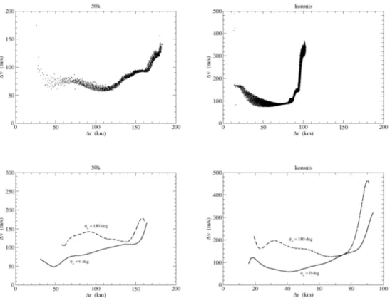
estimate. A more detailed analysis is postponed to a forthcoming work. The analysis of the module of the velocity with respect to the FP reveals other interesting and unexpected features of the SPH models. The SEM assumes a relationship between the velocity, the distance from the IP and the length of the chord from the IP to the surface passing through the fragment (Paolicchi et al., 1989). For the points belonging to any given chord, the SEM requires a strictly monotonically increase ∆v of the ejection velocity as a function of the ∆r distance. This property ensures essentially that the inner fragments do not clash into the outer fragments. We have explored for a comparison the relationship between ∆v and ∆r for the two SPH models, by selecting the fragments located inside a cone having vertex in the FP and axis along a specified direction (φa, θa) (see Fig. 5). The Fig. 6 at the top
shows ∆v versus ∆r for the particles in a cone having θa = 0, that is, the
cone with axis along the line from the FP to the center of the target. The total aperture of the cone is ∆θ = 20◦. In this case ∆v does not increase monotonically from the FP up to the surface, but it has a minimum located more or less halfway between the FP and the opposite surface, then the velocity increases quickly, especially in the case of “koronis”.
We find a similar behaviour by changing the axis of the selection cone, namely when the cone is located at an angular distance θa 6= 0 from the axis
Figure 6: Module of ∆v (velocity respect to FP) versus module of ∆r (distance from FP). On the left the plots corresponding to the field “50k”, on the right to the field “koronis”. At the top relative velocity respect to FP versus the distance from it for particles with initial positions close the line connecting FP to the center of the parent body. At the bottom the same plots for particles selected in off-axis cones with θa = 30◦ and ∆θ = 10◦.
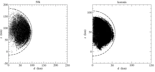
Figure 7: Initial positions in the plane z versus d (see Fig. 3) of the particles involved in direct collisions found by means of the analysis of Sect. 2. The origin of the diagram represents the position of the FP. The dashed line represents the boundary of the parent body.
Figure 8: Initial positions of the colliding particles determined in Sect. 2, having θ ∈ [25◦, 35◦] projected in the plane ∆r versus φ (see Fig. 3). The dashed line represents the boundary of the parent body, while the abscissa axis corresponds to the FP.
Figure 9: Triangle of the impact geometry. The plane of the diagram contains the ini-tial positions A and B of two colliding particles and the impact position (L, F or P ). Dimensions are normalized such that AB = 1. See text for more details.
k. In this case, we find that the plot ∆v versus ∆r is different for different values of the azimuth angle φa of the axis of the cone: ∆v as function of
∆r does not behave symmetrically around the axis FP-center of the target. By changing the orientation of the cone, the minimum of ∆v becomes more or less pronounced, and for a particular value of φa it almost disappears,
especially in the case of “50k”. Moreover, its distance from the FP also changes a little. Fig. 6 at the bottom shows ∆v versus ∆r for two different orientations of the cone. In order to make the figure clearer, we did not plot the points corresponding to each particle, but the mean value of ∆v computed using a running box smoothing technique. The angular distance from the axis k is θa = 30◦, while the total aperture of the cone is ∆θ = 10◦
(that is, the values of θ for the particle inside the cone are in the range [25◦, 35◦]). Two values of the azimuthal angle φaare chosen, being separated
by 180◦, corresponding more or less to the cone orientations for which the minimum of ∆v is more and less pronounced. This asymmetry is presumably connected to the obliquity properties of the original collision.
The properties of the SPH velocity fields discussed above determine the distribution of the initial positions of the particles involved in direct colli-sions. Intuitively, collisions should involve fragments located initially in the region where the variation of ∆v for increasing ∆r is negative. Fragments originating closer to the FP can reach the fragments originating more far away from the FP, but before the distance corresponding to the minimum of ∆v (or just beyond). In Fig. 7 we have plotted the initial positions, in the plane (d, z), of all the fragments involved in direct collisions. From the figure it is evident how the colliding fragments are not randomly distributed
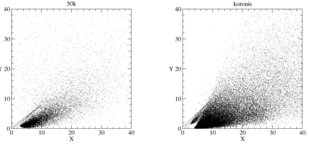
Figure 10: Triangular plots showing the statistics of the impact geometries. The two figures represent the same diagram of Fig. 9 for “50k” (at left) and “koronis” (at right). Each point corresponds to a different pair of colliding particles, and it represents the position of the vertexes of the triangles in Fig. 9. See text for more details.
within the parent body. From Fig. 6 at the top, the fragments that are closer to the axis k should be involved in direct collision if their distance from the FP is between 70 km and 120 km, in the case of “50”, and between 20 km and 80 km in the case of “koronis”. This seems to be confirmed in Fig. 7, looking at the distribution of the dots closer to the vertical axis. Fragments close to the impact point or the parent body’s surface are not involved in direct collisions. Figure 7 is the superposition of all the planes OP P0 (see Fig. 3), but, as we have seen in Fig. 6 at bottom, the velocity field has not a perfect cylindrical symmetry. So, for the particles lying on planes OP P0 with different values of the azimuthal angle φ, the ranges of distances ∆r for which the module ∆v decreases with ∆r are different (and in particular cases they do not exist). As a consequence, the range of distances ∆r containing the initial values of the fragments involved in direct collisions depends on the value of the azimuthal angle φ. Figure 8 shows the plot of ∆r versus φ, for the colliding fragments for which 25◦ < θ < 35◦. The plot (∆r, φ) for “50k” confirms clearly the disappearance of the minimum of function ∆v versus ∆r which is evident in Fig. 6 at the bottom right, when φa = 0◦. Indeed, for
φa = 0◦ the field “50k” has a local minimum around ∆r = 50 km. In Fig.
8 at left, the few dots close to φ = 0◦ and φ = 360◦ and ∆r ∼ 60 km could be a by-product of this local minimum. In the case of “koronis”, Fig. 8 at right confirms the shift of the minimum of ∆v from ∆r = 40 for φ = 0◦, to ∆r = 70 for φ = 180◦ that can be seen in Fig. 6 at the bottom right.
The fact that the ejection velocity (relative to the FP) is not simply a monotonically increasing function of the distance from the FP is certainly a cause of direct collisions. However, also the properties of the deviation
angles play a role. We have analyzed the statistical properties of the impact geometry between the couples of fragments. The purpose is to distinguish in some way the possible different kinds of impact between two fragments, namely cases of head–on impact, with almost opposite velocities, cases of lateral impacts, with nearly parallel velocities, or also cases of pile-up when the velocities have almost the same directions and a faster fragment bumps into a slower one. The classification of the impact geometry depends on the reference system. Here again, we keep the FP reference system, with the above defined system of coordinates.
A useful visual way to characterize the geometry of an impact is to con-sider the shape of a triangle having the line connecting the initial positions of the two fragments as its base, and the position where they collide as the opposite vertex. We do not care here about the size or the orientation in space of that triangle, but only about its shape. For this reason we rescale each triangle corresponding to each pair of colliding fragments in order to have always an identical base of unit length. Then we display all the trian-gles in a cartesian plane (X, Y ) in which all the bases are superimposed to the segment connecting the points (+0.5, 0) and (−0.5, 0). By convention, we place the vertex in such a way that its coordinates X∧ and Y∧ are both
> 0. The coordinate Y∧ is the ratio between the height and the base of the
triangle (see Fig. 9). The position of the vertex in this plane provides a visual representation of the impact geometry. An example is shown in Fig. 9. Points A and B represent the initial positions of the two fragments. A vertex like F corresponds to an impact almost head–on, while a vertex like L corresponds to an impacts almost lateral. The vertex P represents an almost
pile-up impact. The more distant from the base AB P is, the closer it is to the horizontal axis, the more strictly P represents a pile-up (bumping into) impact. Obviously, there are not sharp boundaries between the different types of impact.
If we put on the cartesian plane all the triangles representing the impact configuration of the couples of colliding fragments, we obtain a view of the global distribution of the impact geometries. Really the relevant information is included in the position of the vertexes, which we plot in Fig. 10. All points have a distance from the origin much larger than unity, thus no direct head–on collision is present. Moreover we have very few (if any) points close to the vertical axis, thus very few impacts are purely lateral. The large majority of the points are located in the region of the plot corresponding to almost pile-up impacts. Obviously if all impact were pile-up, all points would lie on the horizontal axis, but this is not the case due to the dispersions of the deviations angles (or in other words, to the non perfect radial orientation of the velocities).
5. Conclusions
Our analysis of SPH models has revealed some important differences with respect to SEMs. We would like to stress that our conclusions are, for the moment, limited only to the two SPH ejection velocity fields that we have at disposal. Our aim is to understand the “hidden” mechanism responsible for the gravitational reaccumulation during the ballistic phase obtained in the particular case reported by Michel et al. (2001). It is not possible for the moment (and it goes beyond our purposes) to extend the conclusions we
reach in this limited analysis to the more general cases of SPH models of asteroid fragmentation. Note, however, that SPH models usually share the presence of massive re-accumulation into many fragments, thus also some other kinematic features like those that we have identified in our analysis might be common. A future general analysis will confirm or falsify this guess.
The distributions of the velocity vectors in the two SPH-simulated ejec-tion fields analyzed in this work suggest that also for them a “fuzzy” ir-radiation point can be defined, similarly to what is assumed a priori as a fundamental hypothesis in the SEM. We find that in the SPH outcomes some deviations from an ideally radial ejection and from a purely monotonic increase of the velocity with the distance from the IP, both make a great difference with respect to the structure of the velocity fields simulated by the SEM.
The SEM also introduces components of the ejection velocity field which are not parallel to the direction from the irradiation point, in order to de-scribe the effect of the rotation of the system after the collision. But even in this case, the SEM excludes the possibility of direct collisions among the fragments. Moreover, by construction the SEM assigns velocities such that fragments closer to the IP move more slowly away than the fragments ejected from initial positions more distant from the IP, automatically excluding the possibility of “bumping into” collisions.
The misalignment of the velocity vectors with respect to the radial direc-tion is not sufficient to fully explain the direct collisions occurring among the fragments simulated by the SPH. A very important role in producing direct
collisions is played by the behavior of the relation between module of the ejection velocity versus distance from the irradiation point. In the velocity fields predicted by SPH, groups of fragments exist such that the assigned velocity decreases with the distance from the irradiation zone. This has as a consequence that some fragments started from inner part of the parent body may reach and collide with fragments moving along the same direction, but originating from other locations. Moreover, a strong correlation between the regions of the parent body where the variation of the ejection velocity is negative for increasing distance from the IP, and the initial locations of the fragments involved in direct collisions has been shown.
We also note that the fact that the properties of the SPH velocity fields determine the distribution of the initial positions of the particles involved in direct collisions tends to confirm recently published results by Michel et al. (2015).
We are not able to give a physical explanation of the relationship between ejection velocity and initial location of the fragment predicted by SPH model. This topic is beyond the scope of this work. We can only imagine the presence of some wave-like behavior in the relation between velocity and position, possibly due to the compression waves produced by the implemented physics in SPH models.
The big question now is whether these features of the ejection velocity fields of the two SPH models that we have analyzed here are per se fully re-sponsible of the significant re-accumulation of the particles into many bodies during the ballistic phase. We know, however, that the reaccumulation dur-ing the ballistic phase was shown not to be sufficient by Michel et al. (2001).
The specific case of Koronis cannot reproduce the observed size distribu-tion if it is not allowed to evolve well beyond the initial expansion considered here. In that case, gravitation reaccumulation becomes very chaotic. A more quantitative and deeper analysis is still needed, because we are aware that the situation might be more complicated. In other words, we can wonder whether the differences in the initial conditions of the ballistic phase - be-tween SPH models and SEM analyzed in this paper are the only one cause of the resulting differences in the re-accumulation outcomes. And are we sure that some properties of the outcomes predicted by the models cannot be the effect of limitations of the numerical techniques adopted to solve these very complex phenomena? We are going to analyze these points more deeply in the next developments of this work.
Acknowledgements
The authors are grateful to two anonymous reviewers for their construc-tive comments.
References
Benz W., Asphaug E. 1999. Catastrophic Disruption Revised. Icarus, 142, 5-20.
Bottke W.F., Durda D.D., Nesvorn´y D., Jedicke R., Morbidelli A., Vokrouh-lick´y D., Levison H. 2005. The fossilized size distribution of the main as-teroid belt. Icarus, 175, 111-140.
Bottke W.F., Vokrouhlick´y D., Broz M., Nesvorn´y D., Morbidelli A. 2001. Dynamical Spreading of Asteroid Families via the Yarkovsky Effect. Sci-ence, 294, 1693-1696.
Carruba V., Burns J.A., Bottke W., Nesvorn´y D. 2003. Orbital evolution of the Gefion and Adeona asteroid families: close encounters with massive asteroids and the Yarkovsky effect. Icarus, 162, 308-327.
Cellino A., Dell’Oro A., Zappal`a V. 2004. Asteroid families: open problems. Planetary and Space Science, 52, 1075-1086.
D’Abramo G., Dell’Oro A., Paolicchi P. 1999. Gravitational effects after the impact disruption of a minor planet: geometrical properties and criteria for the reaccumulation. Planetary and Space Science, 47, 975-986.
Dell’Oro A., Cellino A. 2007. The random walk of Main Belt asteroids: or-bital mobility by non-destructive collisions. Monthly Notices of the Royal Astronomical Society, 380, 399-416.
Doressoundiram A., Paolicchi P., Verlicchi A., Cellino A. 1997. The formation of binary asteroids as outcomes of catastrophic collision. Planetary and Space Science, 45, 757-770.
Love S.G., Ahrens T.J. 1996. Catastrophic impacts on gravity dominated asteroids. Icarus, 124, 141-155.
Melosh H.J. 1989. Impact cratering: A geologic process. Oxford University Press, New York.
Melosh H.J., Ryan E.V., Asphaug E. 1992. Dynamical fragmentation in im-pacts: hydrocode simulations of laboratory impacts. Journal of Geophysi-cal Research, 97/E9, 14735-14759.
Michel P., Benz W., Tanga P., Richardson D.C. 2001. Collisions and Gravita-tional Reaccumulation: Forming Asteroid Families and Satellites. Science, 294, 1696-1700
Michel P., Tanga P., Benz W., Richardson D.C. 2002. Formation of Asteroid Families by Catastropich Disruption: Simulations with Fragmentation and Gravitational Reaccumulation. Icarus, 160, 10-23.
Michel P., Benz W., Richardson D.C. 2004. Catastrophic disruption of pre-shattered parent bodies. Icarus, 168, 420-432
Michel P., Jutzi M., Richardson D.C., Goodrich C.A., Hartmann W.K., O’Brien D.P. 2015. Selective sampling during catastrophic disruption: Mapping the location of reaccumulated fragments in the original parent body. Planet. Space Sci., 107, 24-28
Paolicchi P., Cellino A., Farinella P., Zappal`a V. 1989. A semiempirical model of catastrofic breakup processes. Icarus, 77, 187-212.
Paolicchi P., Verlicchi A., Cellino A. 1996. An improved semi-empirical model of catastrophic impact processes. I. Theory and laboratory experiments. Icarus, 121, 126-157.
Pisani E, Dell’Oro A., Paolicchi P. 1999. Puzzling Asteroid Families. Icarus, 142, 78-88.
Ryan E.V., Melosh H.J. 1998. Impact Fragmentation: From the Laboratory to Asteroids. Icarus, 133, 1-24.
Schmitt L.M. 2001. Theory of genetic algorithms. Theoretical Computer Sci-ence, 259, 1-61.
Vokrouhlick´y D., Broˇz M., Bottke W.F., Nesvorn´y D., Morbidelli A. 2006. Yarkovsky/YORP chronology of asteroid families. Icarus, 182, 118-142. Wiegert P.A. 2015. Meteoroid impacts onto asteroids: A competitor for
Yarkovsky and YORP. Icarus, 252, 22-31.
Whitley D. 1994. A genetic algorithm tutorial. Statistics and Computing, 4, 65-85.