Synthesis, structural and dynamic investigation of chiral metal complexes

Dottorato in Scienze Chimiche

SSD: CHIM/06

Ciclo XXV

A.A. 2010 - 2012

Synthesis, structural and dynamic

investigation of chiral metal complexes

Candidate: Sebastiano Di Pietro

Supervisor: Prof. Lorenzo Di Bari

External Referee: Dr. Marinella Mazzanti

a Salvatore, Lucia e Matteo

ad Arianna, Stefano ed Antonella

I

Contents

INTRODUCTION

Why Lanthanides?

Solution Structure Evaluation

The dual NMR/chiroptical spectroscopies method

Paramagnetic NMR notions ... 7

Chiroptical Spectroscopies ... 13

Paramagnetic NMR

Structural/chemical exchange dynamics ... 17

Structure-spectrum relationships... 22

Dynamical NMR studies in Ln complexes ... 33

Ligand Centered ECD

Electric, magnetic transition moments and rotational strength ... 42

Exciton coupling and DeVoe method ... 50

Metal Centered ECD

The f-f electronic transitions and optical activity ... 57

Static and dynamic coupling mechanisms ... 62

Yb3+ NIR-ECD studies ... 69

Emission Electronic Spectroscopy

Fluorescence spectroscopy ... 73

Circularly polarized luminescence spectroscopy ... 80

References

RESULTS

Pseudocontact shifts in lanthanide complexes with variable crystal field parameters.

S. Di Pietro et al., Coordination Chemistry Reviews 2011, 255, 2810

The structure of MLn(hfbc)4 and a key to high circularly polarized luminescence.

S. Di Pietro et al., Inorganic Chemistry 2012, 51, 12007

Shape-conserving enhancement of vibrational circular dichroism in lanthanide complexes.

III

1

Why Lanthanides?

Lanthanide coordination compounds have aroused large interest in the last decades mainly for their particular spectroscopy properties. Just typing, for example, “Lanthanide Complex” on the Scifinder Scholar research database, it is possible to figure out which are the most representative keywords that characterize the rare earth research field and then their possible applications: on a sample of almost 3000 papers (Figure 1, half of them are less than ten years old), ignoring obvious tags such us “rare earth metals/complexes”, the most recurring concepts in the lanthanide coordination chemistry concern the electronic

spectroscopy (in absorption and emission) properties, followed by molecular/crystal structure

and NMR. Such these three keywords represent, nowadays, either the most important fields of application and the most employed investigation methodologies of rare earth complexes in chemistry, material sciences and biomedicine. With these three keywords, let’s introduce some fundamental issues concerning the rare earth coordination chemistry.

Figure 1. Resulting keywords obtained typing “Lanthanide Complex” in a research database.

Electronic spectroscopy (absorption and emission). The electronic and magnetic

properties of a lanthanide complex are determined and modulated, along the series, by the gradual filling of the 4f orbitals and their unique peculiarities with respect to the d ones in the transition metals complexes. From an inorganic chemistry course, talking about lanthanide is immediately valid the “relationship”

2 Lanthanide f orbitalsburied;

in fact, these orbitals are inner with respect to those with 5- and 6- principal quantum number and display a weak hybridization with them: this determines an outer common frontier for all the lanthanides leading to a similar chemical behavior throughout the series.

Noteworthy, from this atomic structure arises the tendency of a Ln3+ ion (the trivalent state is the most common) to establish mainly electrostatic interactions rather than covalent bonds, with very poor directional character, variable coordination number and small crystal field contact with the ligand. In fact, the electronic terms in a Ln3+ ion, even in a complex, are determined primarily by angular momentum interactions (spin orbit and jj couplings), and not by the influence of crystal field; S (spin angular momentum) and L (orbital quantum momentum) combine together to give the total quantum angular momentum J.

In addition, in a symmetrical environment all ±MJ projections of J (Kramers doublets)

are degenerate. Crystal field may remove this degeneracy to a number of states that depends upon J and especially on the symmetry of the system. Both absorption and emission spectra of Ln3+ have well resolved narrow lines, again for the weak coupling with the environment of the rare earth ions: a closer inspection of these spectral bands reveals a finer structure that contains additional information. This “multiplicity” arises from the different MJ terms for the

spin-orbit coupling (difference of 1000 cm-1) and from sublevels determined by the CFS of each electronic MJ state (of the order of 10 – 1000 cm-1) for the weak interaction f

electron-ligand (Figure 2).

Figure 2. Electronic states of some Ln3+ aquo ions with a closer look on the sublevels arising from the CFS in a eventual lanthanide complex.

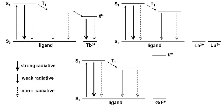
3 While in absorption the f-f transitions are characterized by small , because they are Laporte forbidden in the pure intra-configurational version, almost all Ln3+ are luminescent in an extended range of wavelength (UV, VIS and NIR).

In fact, lanthanide compounds, and in particular complexes with organic ligands, find wide application in light-emitting devices on different levels: from OLED (organic polymers doped with rare earth complexes) to molecular probes in microscopy.

Structure/NMR. The evaluation of the molecular structure is a fundamental step in the

study of a lanthanide coordination compound, not only for the mere identification of an unambiguous species, but also to explain, when is possible, the connection with the specific spectroscopy properties of the system. X-rays diffraction (XRD) is the most used methodology to investigate a structure, but it limited to the solid state and commonly to (relatively large) single crystals; thus it is of little help for understanding the behavior in solution, the phase where almost all the spectroscopy investigations are carried out. In this context, the evaluation of the solution structure becomes of prime relevance, and the

paramagnetic NMR approach results very helpful. In fact, except for La and Lu, all the other

Ln3+ ions have unpaired electrons and are paramagnetic.

To make long story short, the paramagnetism of a Ln3+ ion in a coordination compound determines an interaction between the lanthanide unpaired electron density and the ligand nuclei. At the NMR spectrometer this effect is practically observed in an additional contribution to the chemical shift of an observed nucleus, the paramagnetic shift, and also to the relaxation times (especially shorter T1). From the quantitative analysis of both these

parameters, it is possible to evaluate a detailed solution structure of the system. In addition, thanks to the resonances spreading effect of a Ln3+ ion on the NMR spectrum, it is possible to extend the range of dynamic exchange regimes accessible to NMR.

Obviously, the NMR spectroscopy remains, above all, one of the most important and enduring application field for the lanthanide coordination compounds (just remember the lanthanides shift reagents) as biomedical paramagnetic probes or simply as Gadolinium-based MRI contrast agents.

Just these few keywords highlight the strong connection between the structure of a rare earth complex and its spectroscopy properties, and the designing/developing of new systems may take advantage from the paramagnetic NMR investigation methodology, an approach which will be discussed in detail.

4 Moreover, another interesting aspect is the introduction of chirality elements into a lanthanide complex, in particular thanks to dissymmetric centers/chiral axis into the organic non racemic ligand. This determines some important features:

 Dealing with at least hexacoordinated lanthanide complexes, for some coordination geometries one has to take into account the coordination polyhedron chirality Λ/Δ: when the ligand is itself chiral, its stereogenic elements are conjugated with the Λ/Δ chirality, so as example Λ(RRR) and Λ(RRS) as well as Λ(RRR) and Δ(RRR) are two pairs of diastereoisomers. These aspects, together with the existence of different more or less distorted structures, can give rise to multiple species in solution, sometimes in observable exchange between them.  The possibility to examine the chiroptical properties of the system with the

Circular Dichroism (CD) spectroscopy in a extended range of energies (IR, NIR, UV-VIS), either in absorption (Electronic CD, Vibrational CD), sensitizing the ligand or the metal, than in emission (Circular Polarized Luminescence, CPL).  A non racemic rare earth chiral complex emits circularly polarized light, and the

“enantiomeric excess” of this emission, quantified by the glum,

*

is strictly connected to structural and electronic features. This chirality of the emitted light can be used as another modulation parameter in optoelectronics, to extract further information.

 The presence of C3 or higher axis in the system simplify the paramagnetic NMR

investigation (see later on), in addition, thanks to the isostructurality along the rare earth series, one can extend the structural results obtained for a specific lanthanide element to all the series. This may permit to explain a certain spectroscopic phenomenon observed for a lanthanide thanks to evidences collected from another one.

This thesis summarizes my experience in the investigation of chiral lanthanide complexes and in the research of their structural-properties relationship: this has been realized thanks to a dual methodology based on paramagnetic NMR/chiroptical spectroscopies developed in our team and refined during these last years. Our attention has been focalized onto different chiral systems: stable chelate complexes such as camphorate derivatives and

* 2( ) ( ) L R lum L R I I g I I    _{, where I}

R and IL are respectively the intensity of the emitted right- and left-circularly

5 labile adducts with chiral molecules of natural origin (camphor, carvone, menthol, etc.). On the latter category, a novel spectroscopy effect for the vibrational CD of rare earth chiral

complexes/adducts is pointed out and preliminarily rationalized.

The manuscript is divided in a first part dedicated to our investigation methodologies

flavored with a little bit of theory (paramagnetic NMR, chiroptical spectroscopies, optical

activity of lanthanides systems) required for better understanding the second part, dedicated to published results.†

In conclusion, coming back to the initial issue “Why Lanthanides?” the answer is because this research field has modern, innovative and stimulating applications, from paramagnetic/luminescent probes in biomedicine to dopants for polymers with optoelectronic/photovoltaic uses, and it gives access to investigation methodologies, which provide a detailed picture of many chemical and physical issues involved.

†

All the papers are reprinted with permission from their respective published papers. Copyright 2012-2013 American Chemical Society, Elsevier and Royal Society of Chemistry.

7

Solution Structure Evaluation

The dual NMR/chiroptical spectroscopies method

In this introduction to the chapter I will give some theoretical basic notions on

paramagnetic NMR and the chiroptical spectroscopy applied to chiral lanthanide complexes,

two fundamental tools of a dual method we have developed for the evaluation of the solution structure of rare earth chiral coordination compounds.

As I have already introduced, the paramagnetism of a lanthanide coordination compound, “seen through the eyes” of the NMR spectrometer, represents a valuable instrument to calculate a detailed solution structure of the system. The crude phenomenon observed in a proton/carbon spectra has to be rationalized to get the structural information, that can be contemporarily examined and refined with other techniques, such as the

chiroptical spectroscopies (circular dichroism, CD, in absorption and circularly polarized

luminescence, CPL, in emission) for chiral systems.

Paramagnetic NMR notions

First of all, let’s introduce some basic theory of the lanthanide paramagnetic NMR to better understand this investigation methodology; for a more complete theoretical review see Bertini et al.[1] and for a more applied works see Piguet and Geraldes[2] and Di Bari et al. [3] for chiral lanthanide complexes.

Lanthanide complexes (chiral or not) find a prominent application as auxiliaries in NMR spectroscopy: they induce significant modifications of the analyte spectrum with which they interact. The principal effect resides in the shift of the nuclei resonances of the interacting molecule, commonly referred to as LIS (lanthanide induced shift), accompanied by a broadening of these lines, due to the transverse (T2) component of a phenomenon called LIR

or lanthanide induced relaxation.

The origin of these two lanthanide-induced effects is found in the coupling between the nucleus observed through magnetic resonance and the unpaired lanthanide electrons, the so-called hyperfine interaction. Moreover, different lanthanides that possess a different number of unpaired electrons, exert the same phenomena (shifts and relaxation) with a different “intensity”.

8

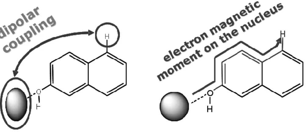
Figure 1. Pseudocontact (left) and Fermi contact shifts (right) origin for an organic moiety coordinated to a Ln3+ ion.

A lanthanide-interacting nucleus (e.g. 1H or 13C) has an observed chemical shift (obs) which is the sum of a paramagnetic term (para) and a diamagnetic one (dia), where the latter is originated from the organic framework electron density, and usually evaluable as the chemical shift of the nucleus in the Lanthanum or Lutetium derivative. The paramagnetic shift is, in turn, the sum of two contributions, called contact (FC, FC or Fermi contact) and pseudocontact shifts (PC, PCS).

obs para dia

   (1)

para FC PC

   (2)

The contact term arises from the probability of finding the electron localised onto the observed nucleus (Figure 1 right); this property is transmitted through covalent bonds and usually can be neglected for nuclei distant more than 4-5 bonds from the paramagnetic centre (unless involved in extensive conjugation). It’s interesting that for three-bond systems, it follows a Karplus-like trend, with a maximum for antiperiplanar arrangements.

On the contrary, the pseudocontact term is directly dependent on the structure and on the magnetic anisotropy of the ion (Figure 1 left) and its dipolar coupling with a nucleus. Large paramagnetic anisotropies are expected when orbital contributions to the ground state is considerable because such contributions are orientation dependent. For lanthanide metal ions, the combination of spin (S) and orbital (L) contributions to the total angular moment (J) (modulated via the spin-orbit coupling) produces considerable magnetic anisotropy when crystal field effects due to coordinated ligands remove the spherical symmetry around the metal. In axially-symmetric complexes we obtain a considerable simplification (some

9 components of the magnetic susceptibility tensor are equal and cancel out), in fact in the presence of a C3 axis (or higher), the pseudocontact shift is described by the useful

McConnel-Robertson relationship 2 3 3cos 1 PC i i i D r     (3)

where the parameter D includes magnetic susceptibility anisotropy and crystal field

parameters,  _{is the polar angle of the considered nucleus and r is the distance from the} lanthanide ion. Equation 3 represents a first example of connection between a spectroscopy parameter as the chemical shift and geometrical ones such as  and r (usually this ratio is abbreviated in G_i, geometrical factor for the i-th nucleus for a specific lanthanide).

Paramagnetism-enhanced relaxation represents the increased rate of nuclear recovery

toward equilibrium determined by very efficient fluctuating magnetic fields generated by the unpaired electrons. Again, electron and nucleus are coupled by dipolar interaction, through two different mechanisms. The nucleus experiences directly the magnetic field generated by the unpaired electron(s), which is called dipolar relaxation; secondly, given its long lifetime, the nucleus senses the average magnetic moment of the molecule, which in turn is responsible for its macroscopic magnetic susceptibility (Curie relaxation). Both these effects follow the trend shown in Equation 4.

1,2 1,2 6 A ( ) = c i i r   (4)

For the dipolar mechanism longitudinal and transverse relaxation rates are equal and

13

10

c s s

 _ 

, the electronic relaxation time. Curie mechanism is temperature dependent (it arises from Curie’s law) and external field dependent. It determines A1≠A2 and consequently

the two relaxation rates are different, with_c_rthe rotational correlation time*. Properly, ri

is the electron-nucleus distance and assumes that the unpaired electron(s) cloud can be effectively described as a point fixed in space (point-dipole approximation). This is usually valid for nuclei 4 Å away and excluding extensive electron delocalisation onto the ligands. In

* _{This can be approximately predicted through the Stokes equation}

3 4 3 R R A M a kT dN kT     , with the

viscosity of the solution, a the radius of the molecule supposed spherical, M_Rthe molecular weight, dthe density and N_Athe Avogadro number.

10 such a hypothesis, ri can be substituted by the nucleus-Ln3+ distance, then, as with the

paramagnetic shifts, also the relaxation rates can give us a connection with structure features of the system in exam.

While the paramagnetic transverse relaxation rates can be tricky to evaluate in a lanthanide complex (additional broadening due to magnetic field inhomogeneity and to partially unresolved scalar couplings may complicate their determination), the longitudinal proton ₁ relaxation rates can be obtained through a simple inversion recovery NMR

sequence: one can easily isolate the paramagnetic contribution to the ₁ using the diamagnetic reference;† we can relate, together with the PCS, the ₁paraof a nucleus to its distance from lanthanide ion obtaining another full set of data (chemical shifts independent) to use in the determination of the solution structure.

The paramagnetic NMR methodology we have refined in the last years, includes different phases: after the real NMR investigation and assignment (see the Paramagnetic NMR part for further details), a second phase envisages the extrapolation of the PCS from the observed shifts, but it’s important to consider some issues:

 We need a diamagnetic reference such us the Lanthanum or Lutetium derivative of the complex.

 We have to consider the presence of free-bound exchange or structural rearrangement equilibria and their rate with respect to the NMR timescale (fast, intermediate or slow) that can complicate our analysis (first of all the assignment phase).

 For certain Ln3+

(see below) we may neglect the FC shifts, mainly because they affect greatly only nuclei (proton, carbon) next to the coordinated donor atom (usually O, N or P) in vicinal and antiperiplanar position to the lanthanide ion (one commonly has to discard them in the investigation of the structure if we can’t assure the correct extraction of the PCS term).

 At any rate, in the literature one can find different separation methodologies for achieving the extraction of the PCS, as will be discussed further below and in great detail in reference [2].

† _again

1 1 1

obs para dia

   or for nuclei not too much close to the Ln3+ ₁dia ₁freeof the free organic molecule/ligand.

11 The most common coordination number, henceforward CN, in lanthanide complexes is 8-9. As I have already pointed out, they are typical hard Lewis acids and the bonding in their complexes is electrostatic and non-directional. As a result, steric factors govern the coordination geometry of lanthanide complexes. The CN may vary along the series reaching 10-12 for La3+ and the other early lanthanides (greater ionic radii), while the capability to expand the CN becomes lessens across the series.

In line with these variable CN, lanthanide complexes can be characterized by a labile axial coordination site, possibly occupied by solvent molecules, water or other ligands. This profoundly alters the crystal field parameters (and ultimately the magnetic susceptibility anisotropy D, see below). Noteworthy, for this modulation of the CN variability, with some Ln3+ it’s possible to observe even the co-existence of hydrated/anhydrous forms for a specific lanthanide in a specific complex: a part is “wet” compound (with axially coordinated water/solvent) and the rest is a “dry” complex; this can also give rise to a intricate situation in relation to the rate of this equilibrium with respect to the NMR timescale. This feature is strictly bound to the high lability of these complexes and so their application as MRI agents, shift reagents and catalysts, and may sometimes be observed with NMR.

The relationship between the magnetic susceptibility anisotropy and crystal field parameters has been investigated by Bleaney[4] and revised by Mironov et al.[5] In the original paper, Bleaney defined _{D as a parameter that represents the magnetic susceptibility}

anisotropy of the lanthanide ion

2 0 j i DC B G (5) 1 ( ) *( 1) ( , ) k i q q k k q i r B e C d r  _{  }    





where C_j is a so-called Bleaney’s factor,B₀2 is the second order crystal field parameter that depends on the distribution of charge around the Ln3+, ( )r in turn heavily dependent on charge and polarizability of donor atoms and their relative positions and distance from the lanthanide ion (Equations 6 and 7). This is a primary source of connection between the spectroscopic issues as the chemical shifts and structural aspects.

12 Once defined the parameter _{D , we can return to the influence of axial coordination of} molecules (ancillary ligands) on the geometry and the spectroscopic properties of the system. As I have just examined, for late Ln3+ the possibility of expanding the coordination number becomes more difficult, so one can observe for the same complex the coexistence of hydrated and anhydrous form along the series. Early lanthanides are usually totally hydrated, instead the late ones, in particular Ytterbium, are anhydrous. Di Bari et al.[6] firstly reported that the

D value can be considered as the sum of two terms:

obs axial ligand

D D D (8)

where axial

D is a function of the nature of the axial ligand and ligand

D is the contribution brought about by the coordination of the ligand. The latter is sensitive to the shape of the coordination polyhedron, assuming different values for different geometries. It’s noteworthy the effect of the presence and the type of coordinated axial molecules on the D final value,

which stems directly from the crystal field theory: in fact the geometrical part ofB₀2 (Equation 7) of a molecule coordinated along the symmetry axis ( 0) may be much larger than the one due to a fragment of the ligand with the same donor atom (oxygen for example).

All the methods – the so-called model-free methods – to separate the contact from the pseudocontact contributions make use of known relationship for i-th nucleus and j-th lanthanide c ij Fi Sz _j    (9) para ij Fi Sz j D Gj i      (10) para ij j i i z j z j D G F S S     (11)

where the terms S_{z j} are rather insensitive to the specific complex and have been calculated throughout the series. Reilley[7] developed a procedure that also permits to underlines possible structural changes along the lanthanide series of the studied complex, by plotting

para ij j z j z j D vs S S 

(Equation 11): a break from a general linear trend (usually two or more linear

13 It’s important to point out again that this method, as other ones, is based on the validity of Bleaney’s theory in particular on the calculated Cj ratios for different lanthanides.

We proposed a new separation method (see the Results part) to reduce the effect of the variation of crystal field parameters, which may be not connected to significant changes in geometry of the system, but rather to axial dynamics or to the small shrinkage brought about from lanthanide contraction.

For the second part of this introduction I will quickly discuss about some fundamental notions on chiroptical spectroscopies, in connection to lanthanide complexes. For an exhaustive and detailed review on the circular dichroism principles and applications there are two recent works by Berova et al in 2007[8] and Pescitelli et al in 2011,[9] and specifically for the circular dichroism of chiral lanthanide complexes see [3] or [10].

Chiroptical Spectroscopies

The definition of circular dichroism is based on the interaction of a chiral non-racemic sample with left and right circularly polarized light (two enantiomeric form of polarized light); the nature of this interaction is diastereomeric, and the difference in absorbance between left and right circularly polarized light of the sample is the circular dichroism (Equation 12).

l r

CD A A (12)

The molar quantity of the circular dichroism is defined trough the Lambert-Beer law as

33000 l r CD c b          (13)

that is independent of concentration c (mol·L-1) and pathlength b (cm). It’s possible to appreciate a non zero CD signal only in correspondence to absorption bands, and it can be positive or negative depending iflis greater or smaller thanr. For organic molecules, usually, most electronic transitions are located in the UV region, and in the regular absorption spectra it’s possible to observe a band, or bands, when the corresponding electronic transition is characterized by a non vanishing electric transition dipole; this is also associated to a CD band (electronic circular dichroism, ECD) if it is allied to an overall roto-traslation of the electronic charge defining an helical path (see later on for further details), which also brings about a non vanishing magnetic transition dipole (m). The integral of a CD band (also called

14 Cotton effect) is proportional to the following scalar product, defined as rotational strength (Equation 14).

d R m

  

   



Then, for a non zero CD signal both the electric and the magnetic transition dipole has to be not orthogonal and not vanishing. For two enantiomers R is equal in magnitude but of opposite sign, which results in exactly opposite CD spectra. All this treatment can be extended to vibrational transitions in chiral molecules/metallic complexes in the IR region (vibrational circular dichroism, VCD) and not only in absorption but also in emission (circularly polarized luminescence, CPL).

Moreover, I recall a very useful rule – called sum rule –: the integral of the CD over the whole electromagnetic spectrum is zero. Usually a non-zero integral in a specific zone may means that in another part of the spectrum one can found other bands that balance it. This aspect will be treated in detail later on, relatively to important electrostatic interaction processes between the Ln3+ ion and the organic ligand.

In the context of organic molecules ECD or CPL, a chromophore is usually a functional group or a combination of several groups with a more or less extended  electron system. A chromophore as in a chiral organic molecule or in a metal complex can be intrinsically chiral or achiral.

As I have reported in the introduction, in lanthanide compounds the chirality of the ligand (with its stereogenic elements) couples with the dissymmetry of the coordination

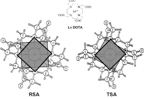
polyhedron. In Figure 2 one can find two common coordination motifs for chiral lanthanide

complexes. With CN = 6 I bring as example a chiral diketonate complex such as the tris

perfluoroalkyl camphorate (Ln(tfc)3 with R = CF3 or Ln(hfbc)3 with R = C3F7) intensively

used in the field of CLSR (chiral lanthanide shift reagents) for NMR, whose polyhedron is a

trigonal antiprism (TA); for CN = 8 I bring as example the DOTMA ligand, a chiral derivative

of the DOTA family (with the tretraazacyclododecane macrocycle scaffold), one of the most popular contrast agents for MRI (molecular resonance imaging); in this case the relative polyhedron is the square antiprism (SA).

Both the polyhedra depicted in Figure 2 have been represented as a regular trigonal antiprism (RTA) or regular square antriprism (RSA): they possess a Cnd or Dnd (n = 3, 4) point

15 arrangement of the chelating bridge connecting the donor atoms. The coordination polyhedron may move away from its regular version, obtaining a certain degree of twist, through a rotation around the symmetry axis of the upper donor atoms plane respect to the lower one (the chelating bridges are then differently tilted). These twisted forms (TTA twisted trigonal antiprism and TSA twisted square antiprism) are otherwise intrinsically chiral, passing from

Cnd to Cn and from Dnd to Dn, losing the improper symmetry elements.

If both the enantiomers of the chiral ligand are present, there may be a further complication, due to the existence of homo- vs. heterochiral species, as it will be discussed in the following section on paramagnetic NMR.

Figure 2.  / stereoisomerism in hexa- (perfluoroalkyl camphorate) and octacoordinated (DOTMA) chiral lanthanide complexes.

Coming back to the investigation of chiral lanthanide complexes with the CD (CPL), the presence of these two type of chiral elements in the system, the ligand chirality and the

coordination polyhedron chirality, gives us the chance to analyze the system from two

different but strictly connected points of view:

 if the ligand contains a suitable chromophore, one can measure the ECD spectrum of the organic framework of the system, ligand centered ECD (LC-ECD); these spectra can be rich of structural details, in particular concerning the relative interaction of the ligand units in space.

16  The other observation window is through the f-f transitions of the rare earth ion (the electronic levels are splitted from spin-orbit coupling and from the crystal field) in absorption, with the metal centered ECD (MC-ECD), or in emission with CPL, which may provide information about the chirality of the coordination polyhedron.

Both these aspects will be treated in two distinct section of this chapter.

Once I have illustrated the basic theory behind the spectroscopic techniques adopted to study chiral lanthanide complexes, the block diagram in Figure 3 exemplify the essence of our dual NMR/Chiroptical spectroscopies investigation method, that will be discussed in detail in the next sections.

Figure 3. Block diagram illustrating all the principal phases of our investigation methodology.

Concluding this introduction, I can now move on to some specific aspects on the investigation of the solution structure of chiral lanthanide complexes starting with the 1H/13C NMR analysis. Later, I will discuss the study of the chiroptical properties of chiral rare earth complexes either in absorption and in emission to point out connections with the solution structure obtained through the paramagnetic analysis.

17

Paramagnetic NMR

Just observing a proton (or carbon) spectrum of a chiral lanthanide complex one can immediately figure out some important aspects of the system:

 thanks to the paramagnetic contribution, all the resonances of the complex are distributed in a large (very large for certain lanthanides) spectral window, then the existence of a paramagnetic complex is easily appreciable.

 The number of paramagnetically-shifted resonances in a proton/carbon spectrum gives a preliminary information on the stoichiometry/symmetry of the complex.  The complex signals are usually easily recognizable (depending on the

lanthanide) because they are strongly shifted and may be broad (they may lose the scalar coupling fine structure); signal overlapping is rare, because they are very spread.

 Consequently, also the free ligand resonances become easily distinguishable; they may arise either from an excess of ligand (or incomplete complexation) or from a free/bound exchange in slow regime.

 Owing to the short T1 it is possible to acquire a spectrum at increased rate, with

short relaxation delay in the pulse sequence; to selectively enhance the paramagnetic signals intensity, with respect to diamagnetic ones due e.g. to free ligand, contaminants, solvent, one can insert a “train” of dummy scans‡ to saturate the signals with longer T1.

Structural/chemical exchange dynamics

I recall a basic notion from any NMR textbook: a dynamic process is slow on NMR timescale if its rate constant k

2 ( )

k   Hz (15)

where  is the separation of resonance frequency between the observed nucleus in the two species in equilibrium. In fast exchange regime, one observes one set of resonances for example during a titration of a ligand with the lanthanide, one follows the spreading of the signals, which asymptotically tend to the ones of the complex.

‡ _{Dummy scans (ds, Bruker) or steady state scans (ss, Varian) contain all of the rf pulses, delays and} gradients used in the pulse program, but the receiver is turned off and data are not collected.

18 In the case of lanthanide complexes, there are at least two parameters which play a special role in the context of dynamic NMR: temperature and the magnetic properties of the Ln3+ ion itself.

On lowering the temperature, there are at least two effects making more stringent the condition expressed in Equation 15: a) there is a well-known decrease of the kinetic rate, k, according to Eyring equation, which is the basis of the so-called DNMR (dynamic NMR) studies and lineshape analysis; b) for paramagnetically-shifted resonances there is an increase of the magnetic susceptibility parameter(s) D of Equation 3, which leads to larger values of .

Moreover, as we have seen in Equation 5, the value of D depends strongly on the lanthanide, according to the Bleaney’s constant CJ (see Table 1), thus D is largest for Dy3+

and very small for Sm3+.

Accordingly the same dynamic process which appears fast at room temperature may easily fall in the slow exchange regime only a few degrees below ambient. Conversely, for a given process, assuming equal rate constants for two different lanthanides, one (with large CJ)

may display a spectrum with two resolved set of resonances (slow exchange) and another (with small CJ) a dynamically averaged one (fast exchange).

A particularly relevant point is to understand if the appearance of one set of paramagnetism-shifted resonances is due to an intrinsic symmetry of the complex or rather to a dynamic symmetrization process. In this case, one can either realize variable temperature spectra (see later on for a quantitative application) or a linewidth analysis: with the first approach we decrease the temperature in order to reach the decoalescence of the signals; there are usually some limitations such as the solubility of the complex at very low temperature, the significant line broadening due to the T-dependence of the transverse relaxation on the Curie law (Equation 18) and to the obvious increase in solvent viscosity, and ultimately the freezing of the solution. With the second methodology instead, one can grossly estimate the “natural” linewidth of some already assigned proton signal, considering all the factors which contribute to it, apart from exchange (Equation 16).

calc dia J coupling dipolar Curie

     

         (16)

In the Equation 16, the diamagnetic contribution can be grossly assessed to 1 Hz; to this one must add an apparent broadening for eventual unresolved multiplicity due to J-couplings; the

19

dipolar and the Curie contribution to the linewidth follows the Equation 4 and it can be

evaluated using these more explicit forms§

2      (17)





In Table 1 I have reported some lanthanide constants.

Table 1. Useful lanthanide parameters for the paramagnetic NMR analysis of complexes. The linewidth are reporter in Hz and calculated with Equations 17-19, the Bleaney’s factors, the Sz expectation values and their ratios are taken from [1]. _sis in ps.

Lanthanide C_Ln S_{z Ln} C_Ln/ S_{z Ln} _s Dipolar Curie (7T) Curie (14.1T)

Ce -6.48 0.98 -6.61 0.5 5.4 0.20 0.81 Pr -11.41 2.97 -3.84 0.5 10.7 0.80 3.2 Nd -4.46 4.49 -0.99 0.5 10.9 0.83 3.4 Sm 0.52 -0.06 -8.68 0.5 0.6 0.0025 0.0099 Eu 4 -10.68 -0.37 - - - - Tb -86.84 -31.82 2.73 0.69 109 43 176 Dy -100 -28.54 3.5 0.82 155 62 249 Ho -39.25 -22.63 1.73 0.54 102 61 250 Er 32.4 -15.37 -2.11 0.85 130 41 166 Tm 52.53 -8.21 -6.4 1.54 147 16 64 Yb 21.64 -2.59 -8.36 0.28 9.6 2.0 8.3

The Curie term (in Hz) is evaluated at two different B0 fields and is calculated assuming the Ln-H distance r = 5 Å and

R = 100 ps. The electronic correlation time τs for the late lanthanides has been taken from [11] and arbitrarily set to 0.5 ps for

the others.

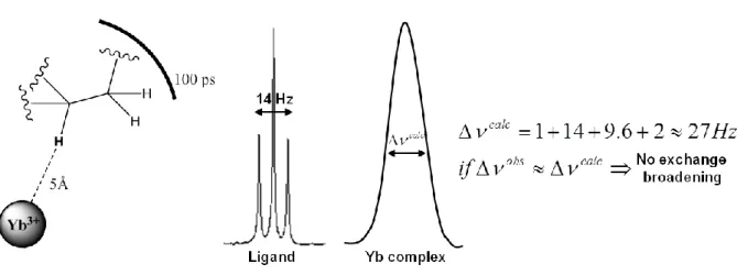
Let’s apply the linewidth approach for the practical example reported in Figure 4: a proton on a methine carbon atom connected to a methylene one with two equivalent protons,

§ _{Here some definitions:} I

 is the Larmor frequency of the I nucleus, _Bis the Bohr magneton, Jis the appropriate quantum number for the lanthanide ion, g_Jthe associated g-factor, _Iis the nuclear magnetogyric ratio for I and k is the Boltzmann constant.

20 is distant 5Å from a Yb3+ ion (distance grossly estimated from a MM optimized structure), considering a R = 100 ps** and an aliphatic geminal coupling (3JH-H = 7 Hz), one can

calculate a calc 27Hz, and we can compare it with the observed one; this may be repeated for other protons to assure a more accurate analysis.

Figure 4. A methine proton analyzed by the linewidth approach to search the presence of a fast dynamic.

The slow exchange is a common situation, in particular for lanthanides with very large paramagnetic shifts (from Eu to Yb excluding Gd). One can observe two sets of signals relative to the free ligand and the complex in chemical exchange between them. If the process is slow according to the definition of Equation 15, but fast enough to allow for magnetization transfer (i.e. k is comparable or smaller to the shortest relaxation rate) one can analyze this process thanks to a 2D EXSY (exchange spectroscopy) map or a simple 1D saturation transfer experiment; in both we follow the magnetization transfer due to a chemical exchange process, instead of through dipole-dipole spin interactions (cross relaxation).

Only for small molecules (short correlation time) one can distinguish cross relaxation cross peaks (same sign as diagonal peaks) from chemical exchange cross peaks (opposite to diagonal) in a NOESY spectrum; for a ROESY this is always true independently from the molecular size, but for lanthanide complexes the ROESY version may be more difficult, because often strong B1 fields†† are required in order to cover the usually very large spectral

width. The most attractive aspect is that the EXSY/NOESY spectra are quantitative. For a simple exchange process the cross peak integral, [AB], and the diagonal peak integral, [AA],

**

Evaluable trough Stokes equation or trough a determination in a diamagnetic derivative (La, Lu) with a 13

C-T1 measurement of a CH system, recorded while saturating

1

H, _r(ps)49.4 T₁1 (s1). †† _B

1 is a continuous radiofrequency field applied for the mixing time interval which spin-locks the y-components of the spin angular moments.

21 can be used to determine the rate constant, where τ is the mixing time of the NMR experiment.

 

 





If the cross peak is small with respect to the diagonal peak, the value of k is small and the above equation approximates to the relationship below that can be solved for k (Equation 21 and 22).

 

 

 

 

If there are more than two species interchanging, the above linear equation can be used for each exchange only when the cross peaks are small (initial rate regime, which can be approximated by using short mixing times ). When the cross peaks are more intense, then matrix analysis is required and this can be done, for example, using the routine EXSY-calc developed by Mestrelab research.[12]

In alternative, to extract the rate constant of a dynamic process (for an intermolecular or intramolecular exchange) in the slow exchange condition, one can observe the variation of the 1D spectrum lineshape on changing the temperature of the sample (lineshape analysis)[13] starting from the spectrum in slow exchange regime at the lowest temperature towards the fast exchange at higher temperature. For a simple process, where the populations of the two interconverting species are equal and when there is no major difference in the relaxation times of the nuclei in the two sites (in paramagnetic system may be a critical point), one can take advantage of a couple of very simple equations relating two notable temperatures and G‡; the following equations will provide G‡ in kJ·mol-1.‡‡

For this calculation, one needs two temperature values:

 The coalescence temperature Tc (i.e. the point when the two lines merge into one)

‡‡ _{We have neglected the scalar coupling between the two exchanging nuclei, which is relevant e.g. when} considering an axial/equatorial equilibrium. When this coupling occurs, or when the two populations are unequal, complete lineshape analysis becomes necessary.

22 ‡ 3 10 ( ) _c ln 2.22 8.31 10 _c ln 1.07 10 c c h G coalescence R T T k T T                 _{ }     _  _     (23)

where  is the difference in Hz between the two lines.

 The temperature Ti where the line broadening starts to become apparent

‡ 3 10 ( ) _i ln 8.31 10 _i ln 1.51 10 i i W h W G initial broadening R T T k T T               _{ }     _  _     (24)

Here W is the extent of the observed line broadening in Hz, obtained as the difference in linewidth between the spectrum at Ti and the ones at lower

temperatures.

It’s clear that B0 inhomogeneity must be very carefully kept under control, possibly

making reference to a standard signal, such as TMS or residual signal/s of the solvent. It should be rather obvious that the initial broadening temperature method is best suited for singlets or for well-resolved multiplets. In any case, temperature control (within 1 K) and sufficient time for reaching stabilization (at least 10 min for each spectrum) are required, as well as accurate shimming before each acquisition.

Another useful experiment in the slow exchange situation is the 1D saturation transfer; typically one can irradiate a paramagnetic signal and observe the resulting effect onto the diamagnetic part of the spectrum to gain some information on the connections between diamagnetic (usually already assigned) and paramagnetic signals (still to assign).

Putting aside the intermediate exchange greatly affected by line broadening,§§ and inert systems, let’s focus in the next section on the analysis of the paramagnetic complex.

Structure-spectrum relationships

Some practical consequences of Equation 3 for chemical shifts and Equation 4 for relaxation rates (in particular I am talking about ₁dipolar

) are depicted in Figure 5 and Figure 6. Let’s analyze each part of these relationships in detail:

 the magnetic anisotropy factor D determines how large is the spectral window of the 1D spectrum; late lanthanides (from Terbium to Ytterbium) all lead to big

§§ _{a problem that we can deal changing temperature, solvent or field, to move this situation toward other} exchange rates.

23 spectral widths, because D _{is proportional to the Bleaney’s constants C}J (Table

1), with a consistent spreading effect onto the proton/carbon resonances, in particular for those nuclei close to the Ln3+ ion. In Figure 5 are displayed three 1H NMR spectra (just simple plots of the experimental proton chemical shifts) of

[Ln(Binolam)3](OTf)3 complex[14] (Binolam =

3,3’-bis(diethylaminomethyl)-1,1’-bi-2-naphthol) for Pr, Nd and Yb; it’s easy to appreciate the connection with the respective C values, _j |CYb| | C_Pr | | CNd |. Choosing a lanthanide with a large D

may help in the assignment process, because all the resonances are perfectly separated.

Figure 5. Comparison between three LnBinolam complexes[14]1H NMR spectra to underline the different spectral windows and so the differentDvalues (the higher signals represent methyl protons).

 The sign of the PCS contribution to the chemical shift is connected to the CJ and

to the 3cos21 _{term of the geometrical factor, where}  _{represents the polar} angle with respect to the major symmetry axis (Figure 6). This term has its maximum positive value (2) with 0,180 deg _{and is zero for} 54.7 deg; this determines (see Figure 6) two zones with opposite PCS sign, which are separated by a conical surface where the PCS is zero (Yb is depicted as example).

24 Simply the sign and the approximate magnitude of the paramagnetic shift gives us information about the relative position of a nucleus with respect to the Ln3+ ion.

Figure 6. Meaning of the geometrical factor (Gi) of the Equation 3 and sign of the PCS considering the Cj and the 3cos2θ-1 factor signs.

 Equation 4 reminds us that a nucleus close to the lanthanide ion possesses a shorter T1 (or a higher relaxation rate 1), than one less proximate. In addition,

the measure of longitudinal relaxation time through inversion recovery sequence may be useful for discriminate and recognize paramagnetic signals (fast recovering to equilibrium) from diamagnetic ones (which stay inverted for longer time). Moreover, it also tell us what repetition time must be used, avoiding signal saturation.

With all these tools one can now approach step by step the assignment phase of the

1

H/13C NMR spectrum of the paramagnetic resonances, with some illustrative examples:

1. The choice of Ln3+ derivatives must be guided by the following considerations: a) the diamagnetic reference should be chosen as La or Lu (or possibly Y) if the paramagnetic one is an early viz. late lanthanide; b) the paramagnetic ion should have a high C_Ln/ S_{z Ln} ratio, in order to ensure maximum PCS vs. FC; c) the linewidth due to dipolar and Curie relaxation should be minimal, compared to the dispersion of the signal, which is effectively measured by the ratio CLn/tot Ln, ;

d) the largest overall PCS should be preferred, because they carry most structural information. Inspection of Figure 7 may guide this choice (y axis represents

25 different measure units, but it’s relevant the comparison between relative values for different lanthanides): the general guideline is “the larger the better” for all the terms depicted. We can appreciate that Pr, Ce and Yb can often be the best choices for small complexes, while for larger molecules (biomolecules, supramolecular systems) Dy and Tb can shift also resonances of distant nuclei (they have highC_Ln). In particular Ytterbium derivatives, when available, represent the best choice (see also the MC-ECD section).

Figure 7. C_Ln (dashed line),C_Ln/ S_{z Ln} (solid line) andC_Ln/_{tot Ln,} (dotted line) plot for the rare earth series referred to the Yb3+ ion.

2. The diamagnetic Lanthanum/Lutetium derivative is fully assigned (1H and 13C) with standard 1D - 2D NMR techniques and proton longitudinal relaxation rates should be also measured with inversion recovery.***

3. A good starting approach to the paramagnetic complex NMR consists in the following steps: a) enlarge the spectral width to ±150 ppm for Yb (which must be changed for a different Ln according to the ratio CLn/CYb); b) use a relatively fast

*** _{The spins are flipped to the –z axis with a}  _{pulse and they evolve}

differently during a following array of delays ( ); a

2

26 repetition rate (300 ms), 4-16 dummy scans (to reduce residual solvent, water and other diamagnetic contaminants signals) and a suitable number of transients to achieve sufficient signal to noise ratio (S/N) especially in the most shifted regions (remember strongly shifted resonances are simple to identify as paramagnetic, but sometimes for their marked broadness one has to raise the vertical scale to identify them); c) run a preliminary inversion recovery with a small number of scans and a rough array of  between 1ms and 1s; d) once one has a rough idea of the relaxation times, set the recovery time to 3 times the longest paramagnetic T1

and run an accurate inversion recovery with a more judicious choice of  (in order to cover the range of the estimated T1’s) and a suitable number of transients to

achieve optimal S/N (for very fast relaxing and strongly shifted signals achieving inversion may be difficult and requires specific tricks to be explained elsewhere); e) re-run the regular proton spectrum with dummy scans and optimal recovery time (3 times the longest paramagnetic T1). In the 0-10 ppm zone, one can

discriminate paramagnetic signals from other ones thanks to their shorter T1. Peak

integrals are still an excellent tool to help our analysis and even though we have lost most of the details of the j-coupling, sometimes one may distinguish singlets from structured signals from the overall shape and linewidth (with the considerations made before).

4. If the relaxation times are long enough (above 10 ms) one may use 2D correlation experiments, with preference for the shortest sequences (e.g. COSY over DQFCOSY). For even longer T1’s standard homo- and heteronuclear assignment

protocols should be fully attempted (although some experiments may fail and some of the peaks may be missing).

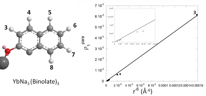
5. Assuming that correlation spectra are not available, a very useful way to tentatively assign a paramagnetic proton spectrum is to take the Ln3+-1H distances from a roughly optimized (MM, possibly by setting the Ln-donor atoms distances to 2.3-2.5 Å) complex structure (thanks to symmetry properties a part of it is enough) and looking for the best linear trend in a ₁paravs r6plot based on the Equation 4.††† An example is shown in Figure 8 for the heterobimetallic complex YbNa3(Binolate)3,[15-18] where the paramagnetic spectrum is easily assigned with

†††

27 this simple approach, obtaining an excellent linear trend and solving a case where integrals or signals fine structure can’t really help the assignment.

6. Every tentative assignment must be checked vs. all available information (e.g. homo or heterocorrelations).

Figure 8. ₁paravs r6plot for the assignment of the YbNa3(Binolate)3 complex. The Yb-H distances are taken from a MM2 optimized structure and T1 data (Yb as paramagnetic choice) are taken from

reference [16].

7. After the assignment of a paramagnetic species, there is the opportunity to “translate” its chemical shifts into others lanthanide ones thanks to an elaboration of Equation 3. 2 , 1 2 1 * Ln para Ln Ln dia i i i Ln C C    (25)

The calculated chemical shifts for Ln2 are compared with the observed ones and critically examined; there will be some discrepancies (again not perfect validity of the Bleaney’s theory or contact term not negligible), but starting from the most shifted resonances (the easiest ones to identify), the others have to follow similar differences/trends as in the calculated shifts than in the experimental ones. The result of this approach is often very good.‡‡‡ In Figure 9 (above) is reported as example the calculation of the Nd derivative resonances with Equation 25 starting from the Yb ones for the already cited Binolam system;[14] noteworthy, almost all

‡‡‡ _{We are considering valid the Bleaney’s theory, neglecting the contact contribution and then the} geometrical factors of the Equation 3 cancels out (same structure).

28 the resonance pattern is well reproduced and it has represented a good guideline for the assignment of this paramagnetic derivative. The protons that are affected by the “largest” error (1-2 ppm) are the two 9a/9b benzylic ones and the 10b of the ethylamino chain. These nuclei are not only considerably close to the Ln3+ ion with a not negligible contact term, but subsequently the solution structure has indicated that the alkyl chain containing the 10b atom lies almost on the change sign surface (this can be visualized in Figure 6 where Binolam were reported as example) with a small PCS value.

At the end of the assignment phase (the carbons signals are assigned in consequence of the proton ones through scalar correlation maps) one can run an

isostructurality test to appreciate the quality of our work; it consists in plotting

the paramagnetic chemical shift of a species (both proton and carbon) against the ones of a lanthanide taken as the reference (usually Ytterbium); a good linear trend indicates that the inter-lanthanides assignment is correct and that isostructurality holds (same geometrical factors) along the series for this complex. The slopes of the _{i Ln,}para₁vs_{i ref,}paraplots are in theory the ratios of the relative Cj, and

the nature of some mismatches can be ascribed to the axial coordination effect illustrated in the introduction part (see later on for a relevant example). In addition, with these plots, proton and carbon atoms affected by large contact shifts are easily pointed out, because the corresponding points in the plot lay far from the fitting line. We should exclude them in the determination of the solution structure, especially if we can’t well isolate their PCS contribution (see next step).

29

Figure 9. NdBinolam exp. and calc. 1H spectrum (above), _{i Ln,}para₁vs_{i Ln,}para₂plot of the Nd and Yb derivatives for the Binolam system (below).[14]

In Figure 9 (below) is depicted as example the _{i Ln,}para₁vs_{i Ln,}para₂ plot for the Binolam system; as one can notice the four nuclei outside the linear trend are considerably affected by contact, especially the two aforementioned benzylic protons and we can’t simply relate the total paramagnetic shift to the PCS. The other effect one can point out from Figure 9 is that the experimental slope (-0.22) is very close to the C_j‘s ratio (-0.206), obviously if we exclude these four atoms from the linear fitting. The excellent linearity in a _{i Ln,}para₁vs_{i Ln,}para₂ plot means essentially that the solution structure is preserved along the series (Nd and Yb are almost opposite) and there are no effects that influence the crystal field parameters, such as the already mentioned different coordination of water (solvent) molecules. This aspect is also corroborated by the similarity between experimental and theoretical

30 slopes, because this system well follows Bleaney’s theory (and this is not a common case).

8. Extracting the PCS from the total paramagnetic term is a very tricky issue. First of all, a central question is: Do we really need to isolate the PCS? In cases where an appreciable contact contribution is solely limited to nuclei (protons and carbons) very close to the Ln3+ ion, while the other ones behave with good/excellent linearity in _{i Ln,}para₁vs_{i Ln,}para₂ plots, one can rely upon the total paramagnetic term without making a large error. This is not always a general case, then the extraction of the pseudocontact contribution becomes considerably important, even because some of these methods allow us to point out the presence of some structural variations along the series. Let’s examine the extended version of Equation 2 for a non-axial system to analyze its fundamental parts (Equation 26 and 27).



 





3 0

1 1

3cos 1 sin cos 2

2 3 para FC PC i j j j j ij ij ij z j zz i xx yy i i I A i A S Tr H N r                   _  _    _     (26)





One can simply go back to the simplified Equation 10 when a C3 axis or higher is

present (_xxj _yyj ). The jterms are part of the susceptibility tensor and together with _z

j

S they depend exclusively from the j-th lanthanide, while the geometrical factors G_iandH_i(the latter called rhombic term) depend only on the i-th nucleus. There are several methods in literature (for a exhaustive treatment see again [2, 3]), and they can be divided into two types, depending on their different approach: one based on the calculation of the anisotropic part of the

paramagnetic susceptibility tensor thanks to an already known reasonable

structural model and the other, model-free methods, instead requires the a priori separation of the FC and PCS contributions. The marked drawback of the first (more theoretical) methodology is the necessity of a previous knowledge of the complex structure, which should best be determined by means of PCS analysis;

31 instead the second methodologies, such as the already exposed Reilley method (Equation 11), found a larger number of applications; high symmetry (presence of at least C3 - C4 axis) again greatly simplifies the problem; moreover, examining a

more complete relationship respect to Equation 11 and grouping some terms of Equation 27 we obtain 2 2 0 2 ( 6 ) para ij Fi Sz _j C B Gj i B Hi      (28)

again one can go back to Equation 10 considering that for axial symmetry system

2

2 0

B  . The Reilley approach consists in factorize Equation 28 with either S_{z j} or C_j(both terms independent from crystal field splitting, Equation 29 and 30).

2 2 0 2 ( 6 ) para ij j i i i z j z j C F B G B H S S     (29) 2 2 0 2 ( 6 ) para z ij j i i i j j S F B G B H C C     (30)

Equation 29 should be used when the _ijparais dominated by the pseudocontact term and Equation 30 when is dominated by the contact contribution. The

resulting para ij j z _j z _j C vs S S  or para z ij j j j S vs C C 

plots give a straight line for the i-th

nucleus for all the j-th lanthanides and each slope permits us to evaluate its PCS term or the FC one. Any deviation from the linearity or abrupt break has always been ascribe to the variation of the B G₀2 _i 6B H₂2 _i structural term (starting from the lanthanide contraction phenomenon). A detailed critical description of Reilley’s method together with a modification proposed during the course of this thesis is presented in the Results part of this work.

9. Once one has extracted the PCS (or determined the simple paramagnetic contribution) and collected the ₁paravalues of the reference lanthanide complex, one needs to optimize the molecular structure of the system (a part of it thanks to the symmetry properties of the system) and to find the one with the minimum difference between experimental and calculated PCS/₁para. The complete