Balancing hydropower production and fluvial connectivity in optimal large scale dam siting on the Mekong river

(1)

SCHOOL OFCIVIL, ENVIRONMENTAL ANDLANDMANAGEMENTENGINEERING

MASTER OFSCIENCE INENVIRONMENTAL ANDLAND PLANNINGENGINEERING

B

ALANCING HYDROPOWER PRODUCTION AND

FLUVIAL CONNECTIVITY IN OPTIMAL LARGE

SCALE DAM SITING ON THE

M

EKONG RIVER

Master Thesis by:

Mattia Gianca Lanzani Dellera Id. 842035 Antonio Pecoraro Id. 842085

Advisor:

Prof. Andrea Castelletti

Co-Advisor:

(2)

(3)

Acknowledgments

We would like to thank Prof. Andrea Castelletti, who gave us the opportunity to work on this thesis project.

We are deeply grateful to our supervisor Dr. Simone Bizzi for the great suggestions and the time that he dedicated us during this thesis.

We also want to express our sincere thanks to Dr. Rafael Schmitt, who helped us in the understanding of the problem and followed the entire development of our work with great advices, also during our period abroad.

Our thanks go also to Prof. Matt Kondolf for letting us fulfil our wish to spend a period abroad at UC Berkley.

We thank our families and friends for their love and support during our entire studies; a particular thank from Antonio goes to Lorenza, for the support, patience and encour-agement.

(4)

(5)

Abstract

The functioning of a fluvial ecosystem is controlled by a complex mix of abiotic, biotic factors and their interactions in space and time. The condition to maintain these inter-actions is the fluvial connectivity, which is the functional exchange pathway of matter, energy and organisms. The construction of dams for hydropower production, flood control and water supply interrupts the fluvial connectivity, affecting in particular sed-iment transport, ecology and natural flow. The Se Kong, Se San, Sre Pok river system (3S river system), in south-east Asia, has the fundamental role of providing sediment to the Mekong Delta. In addition, despite being only 10% of the Mekong basin area (i.e. 81 000 km2), the 3S hosts 42% of the fish species of the entire Mekong, which is the second most biodiverse river in the world. Given the rapid demographic and economic growth of Laos, Cambodia and Vietnam, the 3S has recently become a hotspot of hy-dropower development, the number of dams is expected to grow from the existing 14 up to 42 by 2025.

To allow a sustainable dam development, we combined the 42 dams in different portfo-lios, in order to analyse how their different spatial distributions affect the environmen-tal aspects considered. To pursue our goal, we perform a multi-objective optimization analysis, considering the hydropower production as dam benefit and sediment transport, ecological connectivity and natural flow as dam impacts. To include, for the first time, the sediment transport in an optimization analysis, we developed a computationally ef-ficient large scale sediment connectivity model, based on CASCADE framework. If a basin scale dam planning is adopted from the beginning, most of the indicators allow to reach 65-75% of the hydropower potential (i.e. the total hydropower produc-tion of the 42 dams), limiting the impact on the environmental aspects below 35%. The inclusion of multiple environmental aspects in the optimization allowed to study how a single dam portfolio differently affects the indicators. These differences are more evident for medium hydropower productions. Even if we consider an optimal dam port-folio, developing the 60% of the 3S hydropower potential reduces by 30% the sediment connectivity within the basin. The ecological connectivity of the fish species, instead,

(6)

vironmental aspects, which are differently distributed in the river network. Therefore, its application in river systems that are facing a recent hydropower exploitation, like the Amazon, Irrawaddy and Mekong, can help to adopt an environmentally sustainable dam development to protect fluvial connectivity.

(7)

Riassunto

Le dinamiche di un ecosistema fluviale sono controllate da un complesso insieme di fattori abiotici, biotici e dalle loro interazioni nello spazio e nel tempo. La condi-zione necessaria al mantenimento di queste interazioni è la connettività fluviale, ossia l’interscambio di materia, energia e organismi all’interno del fiume. La costruzione di dighe per scopi idroelettrici, di approvvigionamento e di controllo delle piene interrom-pe la connettività, influenzando, in particolar modo il trasporto di sedimenti, l’ecologia e il deflusso naturale del fiume. I fiumi del sud-est asiatico Se Kong, Se San e Sre Pok definiscono un sottobacino, denominato 3S, del fiume Mekong, il secondo fiume più importante al mondo per biodiversità. Il 3S rappresenta uno dei sottobacini principali per l’approvvigionamento di sedimenti al delta del fiume Mekong e, nonostante costi-tuisca solamente il 10% (i.e. 81 000 km2) del bacino, ospita il 42% delle specie ittiche dell’intero Mekong. A seguito della rapida crescita demografica ed economica di Laos, Cambogia e Vietnam, il bacino del 3S è stato recentemente interessato da un forte svi-luppo idroelettrico: il numero delle dighe presenti sul territorio è destinato a crescere dalle 14 esistenti fino alle 42 progettate per il 2025.

Per una pianificazione idroelettrica sostenibile, abbiamo combinato le 42 dighe ipo-tizzando diversi scenari, in modo da poter analizzare come la loro diversa posizione spaziale vada ad influenzare gli aspetti ambientali presi in esame. Per far ciò, abbiamo applicato un’analisi di ottimizzazione multi-obiettivi a scala di bacino, considerando la produzione idroelettrica come beneficio e l’alterazione del trasporto di sedimenti, della connettività ecologica e del deflusso naturale come impatti. Partendo da CASCADE, modello per il calcolo del trasporto di sedimenti a larga scala, abbiamo sviluppato una sua versione computazionalmente più efficiente, affinchè per la prima volta possa esse-re incluso anche il trasporto di sedimenti in una analisi di ottimizzazione.

La pianificazione a scala di bacino adottata, permette di raggiungere una produzione idroelettrica pari al 65-75% del potenziale totale che si avrebbe con la costruzione di tutte le 42 dighe, mantenendo gli impatti sugli indicatori ambientali al di sotto del 35%. Inoltre, l’introduzione di più aspetti ambientali nell’analisi di ottimizzazione, ha

(8)

per-stato naturale del fiume. Questo sottolinea che gli impatti ambientali non sono dovuti solamente al quantitativo di energia idroelettrica prodotta ma anche alla distribuzione spaziale delle dighe. La metodologia sviluppata in questo studio può essere un impor-tante strumento da utilizzare nei processi decisionali. Essa permette di analizzare un elevato numero di dighe, determinando il loro effetto cumulato a scala di bacino su una moltitudine di aspetti ambientali differentemente distribuiti. Per tale motivo, la sua applicazione in sistemi fluviali interessati da un recente sviluppo idroelettrico, come il Rio delle Amazzoni, l’Irrawaddy e il Mekong, potrebbe aiutare a prendere decisioni che tutelino la connettività fluviale.

(9)

List of Figures

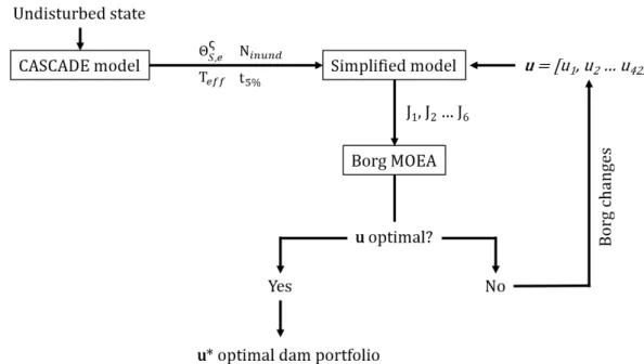
1.1 Flow chart that shows the general methodology adopted in the research. 10

2.1 Dam development in the 3S river basin, including existing, under con-struction and planned dams. The cutout display the 3S basin location within the Mekong river basin (caption and figure adapted from Schmitt, R.J.P.(2017)). . . 13

3.1 Flow chart showing the specific methodology and models adopted in this study. . . 20 3.2 In the example we consider a system composed by 7 dams. In green are

represented the dams selected in the portfolio and in grey the ones not

se-lected. The portfolio corresponds to the decsion vector u = [1, 0, 1, 1, 0, 0, 1]. 21 3.3 The 3 dams partitioned the river network in 4 fragments with specific

volumes (Figure adapted from (Grill et al., 2014)) . . . 25 3.4 Graphical representation of CASCADE framework. A: river network

subdivision in reaches. B: graph representation of the river network by nodes and edges. C: sediment sources identification. D: graph expan-sion in the possible connected nodes. E: representation of the trasport capacity for each grain size and for each reach, indicated by the line width. F: competition corrected transport capacity (smaller than the one from panel E, given by the presence of multiple grain sizes). G: rout-ing of sediment cascades along the river network. H: each edge recives

(12)

3.5 Reservoir routing in CASCADE. A: example of a plan-view and cross-sectional parameters of the inundated reaches by a dam construction. B: subdivision of the reservoir in compartments, as operated by CAS-CADE, and the relative variables. C: sediment accumulation in the reser-voir over a period δt. Siltation requires to update the reserreser-voir bottom, and all the parameters that characterize the compartments. (Figure and caption adapted from Schmitt, R.J.P. (2017)). . . 35 3.6 The dots represent the sediment sources computed in the inverse

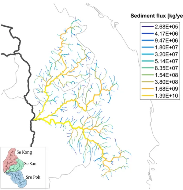
mod-elling. The colors represent the log10of the sediment supply expressed in kg/year. . . 39 3.7 The sediment flux, computed with CASCADE, in the undisturbed state

(i.e. no dams), expressed in kg/year. The Se Kong, Se San, Sre Pok produce 26%, 23% and 51% of the total sediment flux respectively. . . 40 3.8 Flow chart representing the main steps and variables of the Simplified

Model. . . 42 3.9 Matrix containing the input sediment fluxes of each sediment source ς

in each reach e. . . 42 3.10 Sediment flux alteration given by the construction of a dam. . . 43 3.11 Representations of the matrix calculations operated by the Simplified

Model to obtain the final sediment fluxes matrix that is used to compute the indicators. The different panels show: A): the input sediment flux matrix in the undisturbed state; B): in which reach the dam is located; C): how the matrix is modified after apllying the trap efficiency; D): how the matrix is modified after apllying the inundated nodes; E): how the matrix is modified after apllying the 5% threshold. . . 45 3.12 MOEA general procedure: (A) the MOEA algorithm select a random

initial population, in the space of the decision variables, and evaluate its individuals; (B) the algorithm select the individuals that fit better the criteria (i.e. to minimize the objective); (C) the genetic algorithm is ap-plied to the best individuals of the first population to generate offspring; (D) the new population is evaluated; (E) the previous step are repeated until the termination condition is achieved, than the algorithm return the optimal solutions. . . 48 3.13 In the six panels are represented the distributions of the parent and the

offspring produced by the following operators: SBX, DE, UM, PCX, UNDX, SPX. The black dots (•) indicate the parents, while the smaller dots the offpsring (Figure adapted from Hadka and Reed (2013)). . . . 50 3.14 The tournament selection procedure. From the initial population

(13)

com-List of Figures

3.15 The figure displays, during the restart, how the new population is filled starting from the archive of the previous one. The new population is composed by individuals from the previous archive (i.e. portion in white) and by individuals obtained applying mutation on archive individuals (i.e. the portion in grey). The size of the new population depends on the size of the archive and on the ratio γ. . . 52 3.16 Borg main loop (Figure adapted from (Hadka and Reed, 2013)) . . . . 53 3.17 Borg, periodically, checks if the restart mechanism has to be activated.

If yes, the Adaptive Population Size, the Adaptive Tournament Size and the Injection are applied (Figure adapted from (Hadka and Reed, 2013)). 53 4.1 Latin hypercube sampling for the ε parameters. A: First sampling. B:

Second sampling. C: Third sampling. D: Total ε sampling, which is the union of the three prevoius panels. . . 57 5.1 Pareto fronts for different ε settings are represented with coloured dots.

The Pareto front represented with red circles, corresponds to the ε setting chosen for the optimization analysis. . . 62 5.2 Plot of the hypervolume performance in percentage, for each of the 10

initializations of the 30 ε settings, represented by the bar height and colour. The red dots on the background are the maximum hypervolume performance for a given ε calibration. . . 63 5.3 Plot of the optimal solutions obtained for each initializiation in red,

com-pared to the total optimal solutions of the ε setting, represented with black circles. . . 64 5.4 Plot of the Pareto fronts for six different values of NFE to analyse the

convergence of the two-objective optimization problem. . . 65 5.5 Plot of the Pareto front for the two objectives problem in blue, and the

historical dam development in black. The star on the top-right corner is the Utopia point. The four points identified in the historical development are: 1: the current dam development, 2: the dam development before the construction of LSS2, 3: the dam development after the construction of LSS2, 4: the dam development considering the dams already built and the ones under construction. The point shown on the pareto front represents the System Capacity (SC). . . 67 5.6 Spatial distribution of the dams in the 3S basin. Each dam is coloured

according to the probability to be selected in a pareto-optimal portfolio of the Pareto front . . . 69 5.7 A: Subdivision of the Pareto front in Group 1, Group 2, Group 3,

de-pending on the location of the dams selected. B: Representation the dam probability, displayed with the colours, to be included in the portfolios of each Group. . . 70 5.8 In figure are displayed the names of the main dams in the Se Kong, Se

(14)

5.10 Comparison between the Simplified Model and CASCADE, computing for the same dam portfolios the two indicators: Hydropower and Sedi-mentAlteration. . . 76 5.11 On the river network, are displayed the differences in sediment alteration

between the Simplified Model and CASCADE, expressed in percentage. 76 5.12 Plot of the two Pareto fronts obtained running the two-objective

opti-mization once with the Simplified Model (red dots), and once with CAS-CADE (blue circles). . . 78 5.13 Plot of two dam portfolios, one obtained running the two-objective

op-timization with the Simplified Model and the other with CASCADE, corresponding to the same hydropower production. . . 78 5.14 Plot of the Pareto efficient dam portfolios for the six objectives problem

in a seven dimensions space (two dimensions have been used to display the hydropower production). . . 79 5.15 Each panel is a different view of the cube, presented in Figure 5.14,

rotated by 45◦. . . 81 5.16 The Parallel axis plots each portfolio with a line, which intersects the

axes in the corresponding values of the indicators. In figure are presented three parallel axis for different values of hydropower: (A) solutions that have an hydropower production between 30% and 40%; (B) solutions that have an hydropower production between 50% and 60%; (C) solu-tions that have an hydropower production between 90% and 100%. The parallel axis allows to see the performance of a given dam portfolio for all the six objectives, expressed between 0 (worst performance) and 1 (best performance). . . 82 5.17 In Figure we show the dam probability to be included in a dam portfolio

for all the 3 482 optimal solutions obtained in the six-objective optimiza-tion. The probability of each dam is displayed with the different colours. The panel on the bottom left corner displays the dam probability previ-ously obtained in the two-objective optimization (Figure 5.6) . . . 84 5.18 In each panel, the six objectives Pareto front is projected in a

two-dimension space, and is plotted with blue dots. On the x-axes, for all the panels, is displayed the hydropower production, while on the y-axes are displayed the different environmental indicators, in particular A: the

(15)

List of Figures

5.19 In each panel the six-objective Pareto front is projected in a two-dimension space that has on the x-axis the hydropower production, and on the y-axis the different environmental indicators, on both axes the indicators are expressed in percentage. The optimal solutions are plotted with gray circles.. In particular, on the y-axis are displayed in panel A: the SedimentOutlet, B: the SedimentAlteration, C: the EcologicalCon-nectivity, D: MigratoryFishes, E: FlowAlteration. The solutions high-lighted with the different coulours, are the ones that satisfy the constraint EnvironmentalIndicator>80%. The black triangle on the x-axis repre-sents the maximum hydropower production for the group of coloured solutions. . . 88 5.20 The Parallel axis plots each portfolio with a line, which intersects the

axes in the corresponding values of the indicators. In figure are shown the dam portfoloios which allow to preserve 70% of the SedimentAlter-ation indicator. Among these portfolios, we highlighted the one charac-terized by the highest hydropower production. This dam portfolio keep the sediment alteration within the basin below the 30%, affecting sig-nificantly SedimentOutlet, EcologicalConnectiivty and MigratoryFishes indicators . . . 89 5.21 Plot in the Hydropower versus SedimentOutlet space all the optimal dam

portfolios with gray circles, with black dots are plotted the solutions that are common to all the indicators of Figure 5.19 and satisfy the constraint EnvironmentalIndicator>80% for all the indicators. The black triangle on the x-axis represents the maximum hydropower production for the group of common solutions. . . 89 5.22 The solid lines are the Pareto front of each environmental indicator, the

black dashed line is the one of the common solutions. The x-axis is the hydropower production, the y-axis is the environmnental integrity. . . . 90 5.23 A: Dam portfolio for SedimentOutlet=70%. B: Dam portfolio for

Sed-imentAlteration=70%. C: Dam portfolio for MigratoryFishes=70%. D: Dam portfolio for EcologicalConnectivity=70%. . . 92

(16)

(17)

List of Tables

2.1 Distribution of fish species in the three rivers of the 3S according to the

study of Ziv et al. 2012) . . . 12

2.2 Dam database (first part) . . . 14

2.3 Dam database (second part) . . . 15

2.4 Dam database (third part) . . . 16

2.5 Dam database (fourth part) . . . 17

5.1 Trap efficiency, hydropower production and natural sediment flux (i.e. sediment flux in the undisturbed state) of the following dams: Buon Kuop, LSS2, Sekong and O Chum 2 . . . 68

5.2 Trap efficiency, hydropower production and natural sediment flux (i.e. sediment flux in the undisturbed state) of the main dams in Group 1 . . 71

(18)

(19)

CHAPTER

1

Introduction

1.1

General overview

The functioning of a fluvial ecosystem is controlled by a complex mix of abiotic (e.g. temperature, lithology, geomorphology, climatic factors, etc.), biotic factors (i.e. the communities that live in the habitat like human, flora and fauna) and their interaction in space and time. Services provided by fluvial ecosystems can be divided into four broad domains: provisioning services (providing primary resources like water, food, e.g. fishes, timber and sediment for construction (Kondolf , 1994)), regulating services (e.g. climate and flood control, water quality), cultural services (e.g. spiritual, recre-ational, aesthetic), and supporting services (e.g. nutrient cycling, photosynthesis, soil formation) (Millennium Ecosystem Assessment, 2005). Fluvial connectivity is a key condition for the provisioning of most of these services, with connectivity referring to the “functional exchange pathway of matter (i.e. water, sediment, nutrients), energy and organisms”(Ward and Stanford, 1995). Sediment connectivity is a fundamental as-pect directly related to ecosystem integrity and ecosystem services like: access to water resources (Trush et al., 2000), delivery of nutrients and pollutants (Walling, 1983), nat-ural hazard risk (Bechtol and Laurian, 2005) and human livelihood (Habersack et al., 2014).

Since the very beginning, societies built settlements in the proximity of rivers to ex-ploit river ecosystem services. In order to take as much benefits as possible from river resources, human started to build the first fluvial infrastructures like bridges, diversions and dams. Dams have contributed to human development by providing reliable sources

(20)

become even more relevant in the near future. Global energy demand is rapidly in-creasing and climate changes have been recognised as a relevant issue, therefore there is a growing need to fill the energy demand with renewables energies. Hydropower is considered a renewable source of energy (Rosenberg et al., 1997), which, in contrast to other renewables, can cover both the base as well as the peak energy demands (Schmitt, R.J.P., 2017). The number of dams has rapidly grown during the second half of the 20th century driven by the increase of energy and water demands. According to the World Commission on Dams (WCD), in the past half century, on average, two large dams1 have been built per day (Asmal, 2000).

While dams provide immediate economic benefits, they also have negative social and environmental consequences. The World Commission on Dams estimated that 40-80 million people have been displaced by large dams because they were living in areas inundated by the impoundment. Beyond that, few studies were conducted to assess the people affected downstream of dams due to changes in river flow and ecosystem conditions. Richter et al. (2010) conservatively estimated 472 million people living downstream of dams in areas that were impacted by reservoir constructions. For ex-ample, in the Lower Mekong region (Cambodia, Thailand, Laos and Vietnam) it was estimated that about 40 million people (i.e. 71% of the population) directly depend on river and flood-plain fisheries (Sverdrup-Jensen et al., 2002). From an environmental prospective, dams interrupt the fluvial connectivity and cause serious environmental consequences (Richter et al., 2010), that in many cases have led to irreversible loss of species and ecosystems (Asmal, 2000). The long-term impacts include hydrologic and water quality alterations and changes in sediment transport (Williams and Wolman, 1984; Petts and Gurnell, 2005).

The alteration of sediment delivery in the river basin caused by reservoirs, can pro-duce negative effects upstream, within and downstream of the reservoir (Schmitt, R.J.P., 2017). In the upstream part, where most of the sediment is deposited, there is the formation of deltas, which can create flood risk hazard and increase dam backwater effects. Within the reservoir, the accumulation of sediment decreases the reservoir volume, increases maintenance cost for sediment removal from the reservoir bottom, and, finally, increases the risk of dam failure given by the greater static load on the dam. Downstream of the reservoir, the interruption of water and sediment fluxes mod-ifies hydro-morphological and ecological processes. Sediment trapping can impact the rivers immediately downstream of the dam. The water released by the dam is character-ized by sediment-starved water (or “hungry”water), which erode the river bed, inducing incision and channel degradation (Kondolf , 1997); more downstream, at the river delta, water with low sediment concentration can cause delta subsidence and costal erosion (Syvitski et al., 2009). From an ecological point of view, dams, besides preventing the fishes to migrate between different parts of the river system (Branco et al., 2014), also trap most of the nutrients necessary for the maintenance of the downstream ecosystem. To conclude, dams have impacts on many domains of fluvial system functioning. How-ever, the magnitude of those impacts depends on the spatial distribution of the natural

(21)

1.1. General overview

processes in the river basin (e.g. erosional area, migratory fishes path (Jager et al., 2015)), on the characteristics of the dam (e.g. the size of the impoundment, the height, the type of outlet), on its location and on the presence of other dams. For example, the impacts depend if a dam is located along an important fish migration or sediment transport pathway, or if other dams are present upstream or downstream (cumulative impacts of dams (Kondolf et al., 2014)).

To balance benefits and potential impacts of large dams both on people and ecosys-tems, a sustainable hydropower development at basin scale is necessary (Jager et al., 2015). To pursue this goal Richter et al. (2010) proposed a three-step procedure. The first step is to adopt an integrated river basin planning to avoid constructing the dams in the “wrong locations”2_{. An essential key point is to involve river communities in} the planning process through stakeholders surveys, which should reveal the locations that are of critical importance to river-dependent people (Richter et al., 2010). The sec-ond is to design and operate dams in order to minimize the impacts. Important design features can include fish passage structures and sediment sluice gates, while from an operational point of view, the most important feature is the environmental flow release, which must explicitly address the flow volume, timing and quality. Since environmen-tal and social consequences of dams cannot be assessed with complete certainty, the third step proposed is the use of an “adaptive management”, which should include a series of programmes for monitoring, evaluations and adjustments that can be modified along the entire life of the dam according to the different requirements.

Adopting a multi-objective, spatially-explicit-planning approach is an option to assess impacts of dam portfolios on different stakeholders and ecosystem services that are spatially distributed in the river basin (Jager et al., 2015). With dam portfolio we re-fer to a scenario composed by one or multiple dams. Multi-objective analyses have been widely applied in literature for both dam siting and dam removal problems (Kuby et al., 2005; Zheng et al., 2009; O’Hanley, 2011; Ziv et al., 2012; O’Hanley et al., 2013; Null et al., 2014). These studies consider as environmental aspect the impacts on fish species. Very few examples were explicitly considering hydro-morphology as an objective (Schmitt, R.J.P., 2017). However, none of the previous researches considers dam impacts on multiple environmental aspects at the basin scale, even though many indicators that can be derived globally are now available to assess these impacts (Grill et al., 2014).

The purpose of this thesis is to study the conflicts between hydropower production and its impacts on multiple ecosystem services in dam planning. We apply a multi-objective optimization analysis, explicitly including hydro-morphology among the ob-jectives, based on a large-scale sediment connectivity model. Therefore, we are able to capture ecosystem services distribution within the river basin, and find the optimal dam portfolios that maximize the hydropower production, minimizing the environmen-tal impacts.

(22)

(23)

1.2. State of the art

1.2

State of the art

1.2.1 Dam portfolios selection

Due to the growing energy demand and the increase in environmental concerns, many studies about sustainable river basin design have been developed to support complex decision-making processes(Jager et al., 2015).

These studies focus on selecting, from a large number of dams, the most appropri-ate3 _{ones, for which locations and characteristics are already available. Even though} the purposes of these studies are dam siting or dam removal, the methodologies applied are the same.

Kocovsky et al.(2009), using the Habitat Suitability Index (HSI), evaluates the impacts of individual dams on four fish species to prioritize dam removal in the Susquehanna River (USA). In this work, however, nor optimzation is performed nor cumulative dam effects are considered.

A step ahead is made by Schick and Lindley (2007); McKay et al. (2013) who represent connectivity for fish species in a model based on graph theory. The graph theory, in fluvial modelling, represents the river network as a set of nodes connected by edges, where nodes are identified by spatial information and edges represent the process link-ages between nodes. This method allows to capture the spatial distribution of river services in the basin.

To analyse the trade-offs between ecological and economic objectives, an optimiza-tion approach can be adopted (Kuby et al., 2005; Ziv et al., 2012; Null et al., 2014). Given a set of objectives, the impacts of different dam portfolios is evaluated to find the optimal ones.

Adding graphy theory concepts to the optimization analysis, other works are able to find the optimal dam portfolios taking into account also the river connectivity among the objectives (Zheng et al., 2009; O’Hanley, 2011; O’Hanley et al., 2013). However, these applications only consider a single environmental aspect (i.e. fishes) ignoring the multiple impacts of dams on the different river services. As mentioned in Section 1.1, sediment connectivity is one of the key condition for the maintenance of riverine ecosystem, but is rarely accounted in basin scale dam impact.

To partially fill this gap, Schmitt, R.J.P. et al. (2016) developed a graph theoretic-based sediment connectivity model (i.e. CAtchment Sediment Connectivity And DElivery, CASCADE). This framework is applied in the Se Kong, Se San, Sre Pok river system (3S) to find, with an exhaustive search, the dam portfolios, amongst 14 major dam sites, which maximize the hydropower production while minimize the alteration of sediment connectivity.

To conclude, there are many studies about basin scale dam planning to capture the cumulative impact of a multi-reservoir systems on river ecosystem services. Neverthe-less, so far there is a lack of studies that consider multiple environmental impacts (e.g.

(24)

1.2.2 Indicators for environmental performance of dam portfolios

Most studies about dam environmental impacts consider small scale impacts. Only a few studies attempt to evaluate combined effects of multiple dams on ecosystems con-nectivity at large scale (Segurado et al., 2013; Branco et al., 2014; Grill et al., 2014), and even fewer on sediment connectivity (Schmitt, R.J.P., 2017). To estimate the cu-mulative impacts of multiple dams at the large scale, we need environmental indicators that can be easily derived in data-poor settings but that are still reliable for the aim of the study. Our study includes three principal environmental aspects: sediment trans-port, ecological connectivity, and natural flow.

Sediment transport modelling and indicators

Hydro-morphological aspects are rarely considered in integrated water resources man-agement (IWRM) since, modelling sediment transport is complex, computationally ex-pensive at basin scale and the sediment data are often scarce (Merritt et al., 2003). Some hydrological models (e.g. SWAT) and hydraulic models (e.g. HEC-RAS) allow to model sediment transport. On large scale, however, these applications have high computational costs and need a large amount of input data (Merritt et al., 2003; Yalew et al., 2013).

Wild, T.B. and Loucks, D.P.(2012, 2014) developed the Sediment Simulation Screen-ing Model (SedSim) to predict the spatial and temporal accumulation and depletion of sediment in reservoirs, evaluating the combination of three dam portfolios under three different system-wide operating policies. SedSim performs a daily time-step mass bal-ance simulation of water discharge and sediment, however it is not able to distinguish between different sediment grain sizes (Wild, T.B. and Loucks, D.P., 2012).

Recent studies indicate that a graph theoretic approach enables the analysis of envi-ronmental connecntivity (i.e. the transport of water, fishes, sediments and nutrients along the river network) at large scale (Phillips, 2014).

For example, Czuba and Foufoula-Georgiou (2014) adopts a graph theoretic approach to model mud, sand and gravel transport along the Minnesota river. They represent the spatial distribution of processes and process rates in the river network in a graph-based framework in order to obtain the ‚Äúenvironmental response function‚Äù4for a given quantity of interest (e.g. stream flow, sediment and nutrients). In particular, they obtain the sediment flux at outlet for each time step. Their framework, however, does not con-sider multiple grain sizes and returns the sediment flux information only at the basin outlet and not within the basin.

Heckmann and Schwanghart (2013) and Heckmann et al. (2015) propose to apply the graph theory to analyse sediment pathways in small catchments where sediment sources, pathways and sinks are defined using a simulation model for rockfall, debris flow and fluvial processes. This approach allows to have the geomorphological infor-mation in each node of the river network, however, given the large amount of input data

(25)

1.2. State of the art

Schmitt, R.J.P. et al.(2016) developed a spatially distributed modelling framework for sediment transport on large scales and in poor data river systems, CASCADE (CAtch-ment Sedi(CAtch-ment Connectivity And DElivery). In the CASCADE framework, each node has one or multiple sediment sources characterized by a specific grain size and sediment supply. Each source is the origin of a sediment “cascade”that is transported individually along the river network. In this approach, the information of sediment delivery from each source is kept separate along the pathway5and, therefore, unique source sink rele-tionship can be derived.

Two indicators are integrated in CASCADE to evaluate the sediemnt transport: one computes the sediment flux at the basin outlet and the other the sediment flux alteration within the basin.

Ecological connectivity

From the ecological point of view, dams are barriers that interrupt connectivity in both directions, upstream and downstream. The interruption of the ecological connectivty, in the real world, corresponds to the fragmentation of a given habitat, which can dam-age the local species (i.e. fragmentation creates habitat fragments that are no more connected one to the other). Some example of basic indicators for river connectivity alteration are: the number of dams, the river length upstream of each dam, the total river length with altered flow downstream (Anderson et al., 2008) or the portion of the river network accessible from the sea by migratory fishes (Nilsson et al., 2005; Ander-son et al., 2008). More effective indicators, based on the graph-theoretic approach, are also available in litterature. For example, Branco et al. (2014) use the Integral Index of Connectivity (IIC) to quantify the overall connectivity in the basin. IIC is an eas-ily coumputable index, however it evaluates basin fragmentation considering only the number of nodes disconnected, without considering the relative ecological importance of each disconnected node (Segurado et al., 2013). For example, it does not consider if the disconnnected nodes is in main stem or in small tributaries.

Another ecological connectivity indicator is the Dentritic Connectivity Index (DCI) by Cote et al. (2009). DCI is based on the disconnected fragment length in relation to entire network one. Considering the length, however can lead to the same problem that emerged in the IIC. It does not distinguish if a barrier is located upstream or down-stream, in the network, as long as the disconnected fragments have the same length. Based on the DCI indicator, Grill et al. (2014) defined the River Connectivity Index (RCI) replacing the river fragment length with the river fragment volume. In this way, it is possible to weight more the relative impacts of dams located on larger reaches.

Natural flow alteration

Dams are regulated depending on the purpose they are built for (e.g. satisfy water demand, flood regulation, hydropower production). Dam release alters natural flow

(26)

et al., 2014). Quantifying the natural flow alteration can be fully assessed only know-ing the reservoir operation rules. However, this information is rarely available. Given this lack, proxy indicators for assessing natural flow alteration have beeen developed. For example, the Degree of Regulation (DOR) by Lehner et al. (2011) evaluates the percentage of river annual flow that can be stored in a system of reservoirs. A disad-vantage of this indicator is that it does not compute the cumulative dam impact on the entire river network but the alteration is kept separate for each reach.

For this reason, Grill et al. (2014) developed the River Regulation Index (RRI), which takes the information coming from the DOR and weight it according to the reach vol-ume, to get a unique indicator for the basin.

(27)

1.3. Purpose of the study

1.3

Purpose of the study

The state of the art of environmental assessment of dam development, shows a gen-eral lack of studying how different dam portfolios6 can affect different environmental aspects on large scale, especially on sediment. Therefore, the general objective is to study sustainable dam planning through an optimization analysis, considering multiple environmental aspects.

The general objective can be divided in three specific objectives:

I An optimization analysis is a computational expensive procedure. Therefore, the first objective is to develop a computationally efficient simplified model of CAS-CADE framework (i.e. a large-scale sediment connectivity model), to include for the first time the sediment transport in an optimization anlysis, considering a large number of dam protfolios.

II The second objective is to study via optimization the traoffs between dam de-velopment benefits and impacts, considering as benefit the hydropower production and as impact the sediment flux alteration at the basin outlet. This objective was built on the the previous work of Schmitt, R.J.P. (2017), who applied an exhaustive search on a reduced number of dam portfolios.

III The third objective is to run an optimization, including in the previous analysis also the effects on the ecology and natural flow, using recently developed large scale in-dicators. In this analysis , we have considered the hydropower production as dam benefit, while the environmental impacts are measured looking at the alteration of: 1) sediment flux at the basin outlet, 2) sediment flux within the basin, 3) eco-logical connectivity within the basin, 4) ecoeco-logical connectivity with the Mekong main stem 5) natural flow. Moreover, given the different spatial distributions of the environmental aspects within the basin, we analysed whether conflicts between different environmental indicators can emerge in the dam portfolios selection.

To reach our goals, we have developed a methodology that combines a large-scale sediment connectivity model, with an optimization engine (the general formulation is explained in the flowchart of Figure 1.1). In particular, the large-scale sediment con-nectivity model, returns the inputs for a simplified sediment concon-nectivity model, which, given a vector of decision variables (i.e. a dam portfolio), compute the objectives that the optimization engine uses to evaluate if the decision variables vector is optimal or not. If it is not, the optimization engine, automatically changes the decision variable vector and repeat the procedure again, until it finds the set of optimal ones.

(28)

(29)

CHAPTER

2

Case study

The Mekong is the most important river in south-east Asia and one of the main rivers in the continent. The basin has a total surface of about 800 000 km2 and it is shared between six countries, China, Laos, Cambodia, Thailand, Myanmar and Vietnam. At the mouth, the Mekong has an average discharge of 15 000 m3/s with 20-fold seasonal fluctuations from dry to wet season (Kondolf et al., 2014). Besides having the important role as food source for almost 70% of the population living in the area (Sverdrup-Jensen et al., 2002), the Mekong River Basin (MRB) is a biodiversity hotspot for fishes and large-scale fish migrations. With its 877 fish species, 484 of which are living in the delta, the MRB is the second most biodiverse river in the world (after the Amazon river) (Ziv et al., 2012). Other important data that underline its ecological importance are the great number of aquatic endemic species (106 species) (Baran et al., 2013) and the number of long-distance migratory fish species (103 species) (Ziv et al., 2012). In the past decade, due to the rapid demographic and economic growth, the countries in the MRB have been facing an increasing energy demand, leading to a relevant dam de-velopment. The hotspot of this development is the Lower Mekong River Basin (LMRB) (Kondolf et al., 2014), where 133 dams being built, planned or under construction. The tributaries that are most involved in the recent development are the one composing the 3S sub-basin, i.e. the Se Kong, Se San and Sre Pok. The 3S sub-basin has a total area of 81 000 km2 subdivided between Laos, Vietnam and Cambodia and contributes for about 20% (2 890 m3_{/s) to the Mekong discharge (MRC, 2005), and between 6 and} 16% (10-25Mt/year) to its sediment delivery (Wild, T.B. and Loucks, D.P., 2014). Even

(30)

but also from the ecological dimension. Despite representing only 10% of the Mekong basin area, the 3S hosts 42% of the fish species of the entire basin (329 species), 17 of which are super-endemic species (Baran et al., 2013), meaning that they cannot be found anywhere else in the world, and are almost all present in the Se Kong. Ziv et al. (2012), studied how the different fish species are subdivided in the three rivers, the re-sults of their study, in terms of total number of fish species and of migratory species, is summarized in Table 2.1.

In the near future, the total number of dams in the basin will grow from the existing 14 up to 42 (Figure 2.1). In addition to the 14 that are already built, 7 dams are under construction, while the remaining 21 are still in the planning process (Schmitt, R.J.P., 2017). When all the dams will be completed, the hydropower production in the 3S basin could reach 30 463 GWh/year.

Dam development will further impact the fragile ecosystem of the basin, already suffer-ing from climate changes (Ziv et al., 2012). The two sectors that are most impacted by reservoirs are the fish species and the sediment flux. The fishes, besides being the most important source of food for river dependent people (Sverdrup-Jensen et al., 2002), have also a relevant ecological value, and they will be prevented from freely traveling in the basin. The sediment flux, which is the main driver for morphologic equilibrium and delta formation (the Mekong delta is already suffering of subsidence and costal erosion) (Schmitt, R.J.P. et al., 2017), will be highly altered by reservoir construction.

Fish species Migratory fish species

Sre Pok 240 82

Se San 133 54

Se Kong 213 65

Table 2.1: Distribution of fish species in the three rivers of the 3S according to the study of Ziv et al. 2012)

(31)

Figure 2.1: Dam development in the 3S river basin, including existing, under construction and planned dams. The cutout display the 3S basin location within the Mekong river basin (caption and figure adapted from Schmitt, R.J.P. (2017)).

(32)

Code Name River Latitude Longitude COD

L006 Houayho Houayho, Xekong 14.8931 106.6661 1999

L012 Xekaman 3 Houayho, Xekong 15.4361 107.3367 2015

L017 Xekaman 1 Xe Kaman 14.9633 107.1517 2017

L027 Xepian-Xenamnoy Xepian/Xenamnoy 15.0258 106.6056 2019

L028 Xekatam Xenamnoy 15.1354 106.5891 2020

L029 Xekong 4 Xekong 15.5139 106.7878 2022

L030 Nam Kong 1 Nam kong 14.5529 106.7299 2019

L031 Xe Kong 3up Xekong 15.3841 106.7766 2022

L032 Xe Kong 3d Xekong 15.1221 106.8211 2022 L033 Xe Kong 5 Xekong 15.975 106.9306 2019 L061 Xe Kaman 2A Xe Kaman 15.2169 107.4389 2018 L062 Xe Kaman 2B Xe Kaman 15.2753 107.45 2018 L063 Xe Kaman 4 Xe Kaman 15.2244 107.5261 2020 L064 Xe Kaman 4B Xe Kaman 15.3472 107.5358 0

L065 Dak E Mule Xe Kong 15.555 107.0711 2022

L097 Xe Nam Noy 5 Xe Kong 15.1639 106.6686 2013

L098 Houay Lamphan Gnai Xe Kong 15.36 106.4983 2017

L099 Nam Kong 2 Xe Kong 14.4927 106.8532 2018

L100 Xesu Xe Kong 14.7083 107.1764 2022

C001 O Chum 2 O Chum 13.7917 106.9667 1992

C002 Lower Se San 2 Se San 13.5533 106.2 2017

C010 Prek Liang 1 Prek Liang 14.2166 107.2507 0

C011 Prek Liang 2 Prek Liang 14.2833 107.2667 0

C012 Lower Sre Pok 3 (3A) Sre Pok 13.3883 107.05 0

C013 Lower Sre Pok 4 Sre Pok 13.0383 107.45 0

C015 Sekong Sekong 13.7939 106.2544 0

V001 Upper Kontum Se San 14.7111 108.2375 2014

V002 Plei Krong Se San 14.4083 107.8611 2009

V003 Yali Se San 14.2228 107.7931 2002

V004 Se San 3 Se San 14.2167 107.7 2006

V005 Se San 3A Se San 14.1061 107.655 2007

V006 Se San 4 Se San 13.9667 107.5 2010

V007 Se San 4A Se San 13.9333 107.4664 2011

V008 Duc Xuyen Sre Pok 12.1428 108.1006 0

V009 Buon Tua Srah Sre Pok 12.2853 108.0478 2009

V010 Buon Kuop Sre Pok 12.5244 107.9314 2009

V011 Dray Hlinh 2 Sre Pok 12.6769 107.9133 2007

V012 Sre Pok 3 Sre Pok 12.7542 107.8614 2010

V013 Sre Pok 4 Sre Pok 12.8731 107.7806 2010

(33)

Code Name Progress Purpose Dreinage Area Mean Q FSL [km2] [m3/s] [m] L006 Houayho E P 192 9.5 880 L012 Xekaman 3 C P 712 29.6 960 L017 Xekaman 1 C P 3580 175 230 L027 Xepian-Xenamnoy C P 820 42.7 786.5 L028 Xekatam P P 38 12.3 911 L029 Xekong 4 P PC 5400 205 290 L030 Nam Kong 1 P P 1250 42 320

L031 Xe Kong 3up P PAR 5882 240.3 160

L032 Xe Kong 3d P PAR 9700 316.4 117 L033 Xe Kong 5 P P 2518 137 487 L061 Xe Kaman 2A P P 1970 77.5 280 L062 Xe Kaman 2B P P 1740 68.4 370 L063 Xe Kaman 4 P P 265 10.2 860 L064 Xe Kaman 4B P 192 7.4 865 L065 Dak E Mule P P 127 16.1 780 L097 Xe Nam Noy 5 P P 60 3.6 800

L098 Houay Lamphan Gnai C P 140 6.5 840

L099 Nam Kong 2 C P 860 45 460 L100 Xesu P P 1273 77.2 180 C001 O Chum 2 E P 45 2.2 254 C002 Lower Se San 2 C PCF 49200 1306 75 C009 Lower Se San 3 PH PCF 15435 330 140 C010 Prek Liang 1 PP P 917 40.2 275 C011 Prek Liang 2 PP P 580 25.4 495

C012 Lower Sre Pok 3 (3A) PP PCF 25311 713 120

C013 Lower Sre Pok 4 PP PC 13727 378 148

C015 Sekong PH P 28008 1323 63

C016 Lower Se San 1 PH P 11114 385 141

V001 Upper Kontum C P 350 16.7 1170

V002 Plei Krong E PAF 3216 128 570

V003 Yali E PAFN 7455 262 515

V004 Se San 3 E P 7788 274 304.5

V005 Se San 3A E P 8084 283 239

V006 Se San 4 E PAF 9326 328.9 215

V007 Se San 4A E C 9368 330 155.2

V008 Duc Xuyen P PAF 1100 35.7 560

V009 Buon Tua Srah E PAF 2930 102 487.5

V010 Buon Kuop E PAF 7980 217 412

V011 Dray Hlinh 2 E P 8880 241 302

V012 Sre Pok 3 E PF 9410 250.6 272

V013 Sre Pok 4 E P 9568 273 207

(34)

Code Name LSL Live Storage Gross Storage Inundated Area [m] [106m3] [106m3] (at FSL) [km2] L006 Houayho 860 527 674.1 38.3 L012 Xekaman 3 925 108.5 141.5 5.2 L017 Xekaman 1 218 1683 4804 149.8 L027 Xepian-Xenamnoy 745 980 1092 53 L028 Xekatam 890.5 121 126 7.8 L029 Xekong 4 270 3100 10500 170.3 L030 Nam Kong 1 287 505 682.7 21.8 L031 Xe Kong 3up 155 95.1 0 20.8 L032 Xe Kong 3d 111 168.4 0 0 L033 Xe Kong 5 485 1700 3300 32.8 L061 Xe Kaman 2A 275 20.8 20.8 1.5 L062 Xe Kaman 2B 340 333 333 8.6 L063 Xe Kaman 4 840 332.3 0 14.4 L064 Xe Kaman 4B 850 0 0 0 L065 Dak E Mule 756 154 243.1 9.6 L097 Xe Nam Noy 5 780 8.8 9.8 0.6

L098 Houay Lamphan Gnai 800 122 480.5 6.8

L099 Nam Kong 2 437 30.6 166.2 4.2 L100 Xesu 160 26.1 2671 7.2 C001 O Chum 2 251.5 0.1 0 0 C002 Lower Se San 2 74 333.2 1792.5 334.4 C009 Lower Se San 3 118 14528 16900 726.9 C010 Prek Liang 1 260 19.3 0 1.73 C011 Prek Liang 2 480 19.5 0 2.09

C012 Lower Sre Pok 3 (3A) 112 3931 5863 721

C013 Lower Sre Pok 4 146 44 204 33

C015 Sekong 61.5 133.55 0 93.73 C016 Lower Se San 1 140 15.4 100.7 16.3 V001 Upper Kontum 1146 122.7 173.7 8.6 V002 Plei Krong 537 948 1048.7 53.3 V003 Yali 490 779 1037.1 64.5 V004 Se San 3 303.2 3.8 92 3.4 V005 Se San 3A 238.5 4 80.6 8.8 V006 Se San 4 210 264.2 893.3 58.4 V007 Se San 4A 150 7.5 13.1 1.8 V008 Duc Xuyen 551 413.4 1749.78 77.3

V009 Buon Tua Srah 467.5 522.6 787 37.1

V010 Buon Kuop 409 25.6 73.8 5.6

V011 Dray Hlinh 2 299 1.5 2.9 0

V012 Sre Pok 3 267 62.9 219 17.7

V013 Sre Pok 4 204 8.4 29.3 3.8

(35)

Code Name Installed Capacity Production Type [MW] [GWh/year] L006 Houayho 150 487 Reservoir L012 Xekaman 3 250 982.8 Reservoir L017 Xekaman 1 290 1096 Reservoir L027 Xepian-Xenamnoy 410 1748 Reservoir L028 Xekatam 68 380 Reservoir L029 Xekong 4 380 1901 Reservoir L030 Nam Kong 1 150 469 L031 Xe Kong 3up 105 598.7 L032 Xe Kong 3d 100 375.7 L033 Xe Kong 5 330 1201 Reservoir L061 Xe Kaman 2A 64 241.6 L062 Xe Kaman 2B 100 380.5 L063 Xe Kaman 4 54 375 L064 Xe Kaman 4B 0 301 L065 Dak E Mule 130 506 L097 Xe Nam Noy 5 20 124

L098 Houay Lamphan Gnai 84.8 264.4

L099 Nam Kong 2 66 309.5

L100 Xesu 30 286.2

C001 O Chum 2 1 3

C002 Lower Se San 2 400 1953.9 Run-of-River

C009 Lower Se San 3 260 1310.2 Run-of-River

C010 Prek Liang 1 72 324.3 Reservoir

C011 Prek Liang 2 56 259.6 Reservoir

C012 Lower Sre Pok 3 (3A) 300 1201.4

C013 Lower Sre Pok 4 48 220.7

C015 Sekong 190 557.5 Run-of-River

C016 Lower Se San 1 96 485

V001 Upper Kontum 250 1056.4 Reservoir

V002 Plei Krong 100 417.2 Reservoir

V003 Yali 720 3658.6 Reservoir

V004 Se San 3 260 1224.6 Reservoir

V005 Se San 3A 96 479.3 Run-of-River

V006 Se San 4 360 1420.1 Reservoir

V007 Se San 4A 63 296.9 Run-of-River

V008 Duc Xuyen 58 181.3 Reservoir

V009 Buon Tua Srah 86 358.6 Reservoir

V010 Buon Kuop 280 1458.6 Reservoir

V011 Dray Hlinh 2 16 85 Run-of-River

V012 Sre Pok 3 220 1060.2 Reservoir

V013 Sre Pok 4 80 329.3 Reservoir

(36)

(37)

CHAPTER

3

Models and methods

To pursue the goals of our study, we have to solve an optimization problem, in which we want to find the decision variable vector (u) minimizing the indicators (J1, J2, ... , J6).

min

u (J1, J2, ... , J6). (3.1)

In our application the decision variable vector (u) corresponds to a dam portfolio, and is composed by 42 boolean decision variables (i.e. u1, u2, ... , u42), one for each dam, which assume the value 0, if the dam is not selected in the dam portfolio, or 1, if the dam is selected. Even if only 21 dams are actually not built yet, we will suppose that all the 42 dams are subject to the decision, if they have to be built or not. This choice was driven by the fact that most of the dams on the main stem are already built or under construction, therefore most of the environmental aspects are already damaged. Start-ing from the current dam portfolio (i.e. 2016) would reduce too much the degree of freedom of the decision variable set, limiting the analysis..

To evaluate the dam portfolios we introduce six indicators, J1, J2, ... , J6. Two of them want to evaluate dam impacts on sediment connectivity. The model that was available to compute the sediment indicators was a large-scale sediment connectivity model, CAS-CADE framework. However, as previously mentioned in Section 1.3, an optimization analysis is a computationally expensive procedure, and CASCADE is too time con-suming for this application. Therefore, we develop a simplified large-scale sediment

(38)

problem, which has been introduced in a general formulation in Section 1.3. In this section, instead, we will go more in detail in each step of the procedure, following the flowchart in Figure 3.1.

We started from running in the undisturbed state (i.e. without any dam) CASCADE model, which provides the information about: sediment fluxes (Θς_S,e), dam trap ef-ficiency (Tef f), size of the dam impoundment (Ninund), and sediment flux threshold (t5%)1. These variables, are given as input to the Simplified Model, together with the decision variables vector u. The Simplified Model, allows to compute the indi-cators J1, J2, ... , J6, that are given to the optimization engine, Borg. Borg, is a Multi-Objective Evolutionary Algorithm (MOEA), that, from the indicators, evaluates if a dam portfolio is optimal or not. If it is not, it automatically changes the values of the decision variables u1, u2, ... , u42, and restarts the procedure just described until it finds the optimal dam portfolio u∗.

Figure 3.1: Flow chart showing the specific methodology and models adopted in this study.

3.1

Decision variables

As previously mentioned, in our problem, the decision variables vector is a composed by 42 elements, one for each dam. The decision variable uithat composes the vector, is a boolean variable, that assumes the value 0 if the dam is not selected in the portfolio, and 1 if it is selected. For example, considering the dam portfolio in Figure 3.2, in which in green are represented the dams selected in the portfolio and in grey the ones not selected, the decision variables vector would be:

(39)

3.2. Indicators

others u2,5,6 = 0.

The inclusion of a dam in a portfolio, means that its effect on fluvial connectivity are activated in the model, through the trap efficiency and the impoundment effects.

Figure 3.2: In the example we consider a system composed by 7 dams. In green are represented the dams selected in the portfolio and in grey the ones not selected. The portfolio corresponds to the decsion vectoru = [1, 0, 1, 1, 0, 0, 1].

3.2

Indicators

To evaluate the benefits and the impacts of a dam portfolio we use a set of six indi-cators, one to evaluate the dam benefit as the driver for the dam development, five to evaluate the dam impacts on three main environmental aspects: sediment, ecology and natural flow. The indicators assessing the sediment aspect are model-based (i.e. based on sediment processes) while the indicators assessing the other environmental aspects (ecosystem and natural flow) are graph-based (i.e. they are proxy indicator since we do not include an ecological model).

3.2.1 Hydroelectricity

Among the dam benefits (e.g. hydropower porduction, flood control, water supply), we choose to focus our analysis on the hydropower production.

Hydropower production

In our case study, the annual hydropower production for each dam, expressed in GWh/year, is given by the Dam Database from the Mekong River Commission (MRC). Since the indicator takes into account the hydropower production of a given dam portfolio, we

(40)

J1 = N X i=1 Gi [GWh/year], (3.2) where

N is the number of dams in the portfolio;

Gi is the annual hydropower production of dam i [GWh/year]. In the next chapters, we will refer to J1 _{as “Hydropower”.}

3.2.2 Sediment

As mentioned in Chapter 2, the 3S river system is very important for the sediment de-livered to the Mekong, its contribution, in fact, is between 6-16% (i.e. 10-25 Mt/year) of the total sediment flux (Wild, T.B. and Loucks, D.P., 2014).

In this study, we have adopted two indicators, proposed by Schmitt, R.J.P. (2017), to evaluate the sediment delivery alteration: sediment flux at the river basin outlet (i.e. external sediment connectivity) and total sediment flux alteration within the river basin (i.e. internal sediment connectivity). Schmitt, R.J.P. (2017) implemented these two in-dicators, based on CASCADE approach (see Section 3.3), to evaluate dam impacts on sediment delivery.

Sediment flux at the river basin outlet

This indicator is obtained summing up, a the basin outlet, all the sediment fluxe coming from sediment sources spatially distributed in the basin (developed by Schmitt, R.J.P. (2017)). The sediment flux (ΘS) for a given dam portfolio is calculated using the Sim-plified Model (see Section 3.4.

J2 = N X i=1 Θi_S,Ω [kg/year], (3.3) where

N is the number of sediment sources;

Θi_S,Ω is the sediment flux of the sediment source i at the basin outlet Ω [kg/year]. This indicator considers only the sediment flux at the basin outlet. Comparing the value of the indicator obtained with a given dam portfolio with the one obtained in the undisturbed state, we can evaluate the reduction of sediment flux coming from the basin. However, this indicator does not take into account the impacts on the local sedi-ment flux (i.e. in each reach).

(41)

3.2. Indicators

Total sediment flux alteration in the river basin

This indicator evaluates the difference in each reach between the sediment flux in the undisturbed state and the one with the dam portfolio considered (developed by Schmitt, R.J.P. (2017)). Then the difference in each reach is weighted by the corresponding reach length to aggregate the impacts in just one value for the entire basin. Considering the total sediment flux alteration, it is possible to evaluate the dam impacts on sediment flux within the river basin.

J3 = ( N X

i=1

∆Θi_S,e) × L [kg*L/year], (3.4)

where ∆Θς_S,e = Θς_S,e(bd) − Θς_S,e(pd) [kg/year], where

∆Θς_S,eis a matrix2 _{cointaining the difference between sediment fluxes before and post} dam construction for each reach e and for each sediment source ς [kg/year];

Θς_S,e(bd) is a matrix containing the sediment flux of each source ς in each reach e in the undisturbed state (bd=before-dams) [kg/year];

Θς_S,e(pd) is a matrix containing the sediment flux of each source ς in each reach e with the dam portfolio selected (pd=post-dams) [kg/year];

∆Θi_S,e is a vector cointaining the difference between sediment fluxes before and post dam construction for each reach e [kg/year];

L is a vector containing the reach lengths [m]. In Equation 3.4, the first term (ΣN_i=1∆Θi

S,e) sums for each reach, e, all the differences in sediment fluxes coming from different sediment sources i. Therefore, the result of this term is a row vector, with a length equal to the number of reaches, that has to be multiplied (i.e. vector product) by the vector of the reach lengths.

The higher is the indicator value, the higher is the sediment alteration inside the river network.

In the next chapters, we will refer to J3 as “SedimentAlteration”.

3.2.3 Ecology

The 3S river system is very rich in fish biodiversity. In fact, although the 3S watershed represents only 10% of the Mekong one, the 3S hosts 329 fish species, 42% of the total spices existing in the entire Mekong area.

In this study, when we will refer to ecology, we will consider the impact only on the fish species. The following indicators are not based on a model but on the graph theory, so they are proxy indicators and not process based as the two for the sediment.

(42)

connectivity: the River Connectivity Index (RCI) and the Migratory fishes connectiv-ity, respectively. With these two indicators, we will account for the barrier effect of dams, which prevents the fish species to migrate in the river basin. Dams will be con-sidered completely impermeable to the fish species in both directions, from upstream to downstream and vice versa (i.e. no fish passage).

River Connectivity Index (RCI)

In order to evaluate the fish habitat fragmentation within the river basin, we used the RCI by Grill et al. (2015). This indicator is designed to evaluate dam cumulative im-pact on fish species. The basic concept of the RCI is that a dam, as a barrier, partition the river network into fragments that are not connected anymore one to the other (Fig-ure 3.3).

The river connectivity index is the sum of the ratios between the volume of the frag-ment i squared, over the total basin volume squared.

J4 = N X i=1 V_i2 V2 tot · 100 [%], (3.5) where

N is the number of fragments;

Viis the river volume of fragment i [m3];

Vtotis the volume of the entire river network [m3].

Both volumes are calculated multiplying the reach length by its witdh and depth. The channel is assumed to be prismatic, therefore, witdh and depth are constant along each reach. The length is extracted from the river network, the width is computed using a scaling law based on the drainage area and the energy slope (see Equation 3.29), the depth is computed using the 1.5 year return period discharge, which corrisponds to the bankfull conditions (its computation is included in CASCADE framework, see Section 3.3.6).

The RCI measures the ecological connectivity of the river network, if the RCI value is 100%, the river basin connectivity is undamaged.

In the next chapter, we will refer to J4 as “EcologicalConnectivity”.

Migratory fishes connectivity

(43)

3.2. Indicators

J5 = VΩ [m3], (3.6)

where

VΩ is the volume of the most downstream fragment (i.e. the fragment connected with the outlet Ω) [m3].

The larger is the volume accessible, the larger is the habitat the migratory fishes have available.

In the next chapters, we will refer to J5 _{as “MigratoryFishes”.}

Figure 3.3: The 3 dams partitioned the river network in 4 fragments with specific volumes (Figure adapted from (Grill et al., 2014))

3.2.4 Natural flow

In the previous Section 3.2.3 we presented two indicators to assess the barrier effect of dams. In this section, instead, we will present an indicator, based on the graph theory, to evaluate dam impact, on ecosystem processes, resulting from natural flow alteration. We adopted the RRI by Grill et al. (2014), who expanded the Degree of Regulation

(44)

J6 = N X i=1 DORi· rvi Vtot [%], (3.7) where DORi = M P j=1 sj Di · 100 [%], where

sj is the storage capacity of dam j [m3];

Di is the total annual discharge flowing through the reach i [m3];

DORiis the potential effect of dams j = 1, ..., M on natural flow of reach i [%]; rvi is the river volume of reach i [m3];

Vtotis the volume of the entire river network [m3].

The first step is to calculate the DOR, summing up the storage volume (sj) of all the reservoirs upstream of a reach i and dividing it by the total discharge (Di), flowing through the reach in one year. The DORi, therefore, measures how much water the reservoirs subtract from the natural flow of reach i. Usually 10% is the threshold to mark evident changes in the natural flow regime (Lehner et al., 2011).

To obtian the RRI, the DOR is multiplied by the volume of reach i in percentage (rvi/Vtot). Using the river volume as weight, it allows to consider also if the altered flow regards a small or a large volume.

The total annual discharge Di has been computed as the annual average of the hydro-graphs available in each reach, that for the 3S is a 20 years record. The hydrograph is extracted from the pre-processing of CASCADE (to see the extraction of the hydro-graph, see Section 3.3.6.

(45)

3.3. CASCADE modelling framework

3.3

CASCADE modelling framework

CASCADE (CAtchment Sediment Connectivity And DElivery) is a large-scale sed-iment connectivity model recently developed by Schmitt, R.J.P. et al. (2016). This approach combines graph theory concepts with sediment transport modelling. The sed-iment delivery coming from multiple sources is described through individual transport processess, called “cascades”. This allows to keep the information about provenance and destination, of a single sediment source, disaggregated along the river network. In our application, the sediment indicators, i.e. SedimentOutlet (J2) and SedimentAl-teration (J3), have to be computed using a large-scale sediment connectivity model. CASCADE is too computationally expensive for an optimization analysis. Therefore, the indicators cannot be computed through this model. CASCADE, however, is used as the starting point for the development of a simplified large-scale sediment connectivity model, the Simplified Model (SM). Moreover, a preliminary run of CASCADE in the undisturbed state (i.e. without dams) provides the variables Θς_S,e, Tef f, Ninundand t5% (introduced in Figure 3.1 and further explain in Section 3.4), which are the inputs used by the Simplified Model to compute the sediment fluxes in the basin.

In Sections 3.3.1, 3.3.2, 3.3.3, 3.3.4, 3.3.5, we go through the main procedures imple-mented in CASCADE framework, while in Section 3.3.6 we describe the implementa-tion of CASCADE in the 3S basin by Schmitt, R.J.P. et al. (2016).

3.3.1 CASCADE approach

In Figure 3.4, are summarized the main aspects, used by CASCADE framework, to model sediment delivery in a river basin. The starting point is the river network (Fig-ure 3.4(A)), that has to be transformed in a directed acyclic graph (Fig(Fig-ure 3.4(B)), composed by nodes (identified by arabic numbers), representing river confluences or connections, and edges representing river reaches. For each reach, one or multiple sources (indicated with roman numbers) are identified (Figure 3.4(C)). For instance, in correspondence of the reach 2 we have sources II and III. Each source is characterized by a grain size, visualized with the dot size, and a sediment supply. To keep track of each sediment source along the river network, the graph from Figure 3.4(B) has to be expanded into the one in Figure 3.4(D), so that, the information of different cascades is kept separate. The expanded graph represents the possible path of each sediment source in the river network (i.e. the possible connected nodes). For each reach and for each sediment source, the transport capacity, which is the energy available for sed-iment entrainment, is computed using standard sedsed-iment transport formulas, based on the source grain size, on local geomorphology and on local hydraulic conditions. In Figure 3.4(E), the transport capacity is visualized by the line width. As we can no-tice, the transport capacity can change along the cascade path, and, since it depends on the grain size, it is different for cascades active in the same reach. For example, in reach number 2, source number III has a higher transport capacity than source num-ber II, since it is characterized by a smaller grain size. However, in Figure 3.4(E), the

(46)

through the “competition”. The competition corrected transport capacity is displayed in 3.4(F). The differences between the two transport capacities, can be seen, for example, in reach 5, where all the sources IV, V and VI experienced a lower energy available. As displayed in Figure 3.4(G), along a cascade, no additional sediment is taken up, but only deposition can be observed, otherwise no unique connectivity information could be derived. Sediment of a cascade can deposit if the sediment input in the reach is greater than the local transport capacity, or if the cascade has to be routed through a reservoir, in which we have a drop in the energy available for entrainment. A sediment cascade is interrupted if all his initial supply has deposited, for example sources I and II are both interrupted in reach 3. The reaches in which deposition is observed, are defined as sinks. In Figure 3.4(G) it can be observed that reach 2 is a sink for cascade I, reach 3 for sources I, II and III, and reach number 5 is a sink for cascades III, IV and V. Therefore, we can conclude that, a reach can have the function of sink for multiple sediment cascades. The peculiarity of CASCADE framework is that the information is kept disaggregated for all the sediment sources and for all the reaches, as a conse-quence, sediment provenance and connectivity information can be derived in any node. In particular the output of the model is a matrix, that we further refer as Θς_S,e, in which the sediment fluxe for each cascade ς3_{in each reach e is stored.}

3.3.2 Conventions and symbols

In this section, we introduce some of the conventions and symbols that are used in the following chapters. As previously mentioned, the river network has to be split in a directed acyclic graph composed by edges (indicated with e in the set of all the edges E) and nodes (indicated with n in the set of all the nodes N ). In this case study, we have one source for each reach (i.e. no multiple sources like it was presented in Section 3.3.1) indicated with ς ∈ S, where ς indicates the single source and S is the total num-ber of active sources. Each source ς, has a characteristic grain size dς, and is the origin of one and only one sediment cascade γ ∈ Γ. Where γ is the single cascade, and Γ is the total number of cascades, which has cardinality g, and, in this case, it is equal to the number of active sources S. Each sediment source, is the starting point of a pathway κ ⊆ E, which is the set of the edges from the source ς, till the basin outlet Ω (if it is not interrupted because of deposition or by the presence of a reservoir). Therefore, a general path of a source, is indicated as κς. Some examples of connectivity information that can be derived from CASCADE are the total cascades connected to a certain edge e, which will be expressed as Γe ∈ Γ, and the sources that are connected to the edge e, that can be written as Se ∈ S. Some more variables that will be used in the following sections, and that can be useful to introduce at this point are: the transport capacity QS, which, if referred to a general cascade γς in the edge e, will be expressed as QSςe; and the sediment flux Θ, which, if referred to a cascade γς in the edge e, is written as Θςe.

(47)

3.3. CASCADE modelling framework

Figure 3.4: Graphical representation of CASCADE framework. A: river network subdivision in reaches. B: graph representation of the river network by nodes and edges. C: sediment sources identification. D: graph expansion in the possible connected nodes. E: representation of the trasport capacity for each grain size and for each reach, indicated by the line width. F: competition corrected transport capacity (smaller than the one from panel E, given by the presence of multiple grain sizes). G: routing of sediment cascades along the river network. H: each edge recives sediment from multiple cascades, defining sediment flux, provenance, and sorting; and thereby connectivity of an edge. (Figure and caption adapted from Schmitt, R.J.P. et al. (2016))