Runtime support for stencil data-parallel applications on multicore architectures

(1)

Università di Pisa and Scuola Superiore Sant’Anna

Master Program in Computer Science and Networking

Corso di Laurea Magistrale in Informatica e Networking

Master thesis

Runtime support for stencil

data-parallel applications on

multicore architectures

Candidate

Supervisor

Paolo Giangrandi

Prof. Marco Vanneschi

(2)

List of Figures

1.1 Sample execution of application with compile time support . . 8

1.2 The dependency graph managed by our support . . . 9

2.1 Stencil for computation in listing 2.2, with M = 3 and i = 0 . 16 3.1 Dependency graph for computation in listing 2.2, with M = 3 18 3.2 Dependency graph for an example computation . . . 19

3.3 Support working overview . . . 22

3.4 Dependency graph faithful implementation . . . 24

3.5 Dependency matrix . . . 26

3.6 Map with barrier implementation overview . . . 28

3.7 Dependency graph for computation in section 2.4, with M = 3 33 3.8 Support abstract view . . . 37

4.1 Titanic topology . . . 43

4.2 Andromeda topology . . . 44

4.3 Representation of cholesky algorithm . . . 46

4.4 Sample execution of application with compile time support . . 47

4.5 Stencil for Cholesky Decomposition application . . . 48

4.6 Sample execution of application with our runtime support . . 50

4.7 Completion time of the different implementations for scenario 1 on titanic. . . 52

4.8 Scalability of the different implementations for scenario 1 on titanic . . . 53

(5)

List of Figures 4

4.9 Completion time of map with barrier with different values for

Q on titanic . . . 57

4.10 Completion time of the different implementations for scenario 1 on andromeda . . . 58

4.11 Scalability of the different implementations for scenario 1 on andromeda . . . 59

4.14 Completion time of the different implementations for scenario 2 on andromeda . . . 62

4.15 Scalability of the different implementations for scenario 2 on andromeda . . . 63

4.18 Jacobi’s virtual processors in action . . . 67

4.19 Jacobi dependency graph . . . 68

4.20 Tridiagonal solver’s virtual processors in action . . . 69

4.21 Tridiagonal solver dependency graph . . . 69

4.22 Completion time for scenario 1 of Jacobi . . . 71

4.23 Completion time for scenario 1 of tridiagonal solver . . . 72

4.24 Virtual processors fetched at once . . . 74

4.25 Completion time of map with barrier with different values for Q 75 4.26 Completion time for scenario 2 of Jacobi . . . 76

4.28 Completion time for scenario 3 of Jacobi . . . 77

(6)

Listings

2.1 Sequential computation example . . . 15

2.2 Virtual Processor for the example computation. . . 16

3.1 AbstractProcessor main loop . . . 37

3.2 JobFactory with depency matrix fetching function . . . 38

3.3 JobFactory with depency matrix finalizing function . . . 38

3.4 JobFactory with frontier finalizing function . . . 39

3.5 JobFactory with map with barrier fetching function . . . 40

4.1 Cholesky decompositino algorithm. . . 45

4.2 Our benchmark function . . . 66

5.1 Virtual Processor function for a stencil needing buffering . . . 82

(7)

CHAPTER

1

Introduction

This work will focus on studying and developing an optimized runtime sup-port for a particular set of parallel applications: stencil-based data-parallel applications. Data-parallel computations are computations parallelized by partitioning the input data and replicating the functionalities. During 2011 Di Girolamo [10] already did some work on MAP data-parallel applications, that are computations without data dependencies between different parti-tions of data. This work aims to further study and optimize such work, especially taking into account stencil-based parallel applications: data-parallel applications with data dependencies between the different partitions of input data.

We will rely on the Virtual Processor approach [27]: a virtual processor is a module that takes ownership of a data partition and runs a sequential algo-rithm.

With this work we analyse in details the characteristics of generic stencils for virtual processors, define a generic interface to describe this kind of applica-tions and implement a number of supports to actually perform the compu-tations.

Finally we tested our support implementations both on real-world tions and on some benchmarks and noticed that in some cases the applica-tions implemented over our support can perform better than eavily-optimized hand-written applications.

(8)

7

The next step of this work will be to define a cost model for our support and its several implementations, that could be used to understand what we can expect from a dynimac support and which support implementation would fit best to model an application.

A dynamic support for stencil data-parallel applications

Usually, data-parallel applications statically partition the virtual proccessors, assigning them to the actual processing units at compile time. This strategy introduces very little overhead, but has a few limitations:

1. virtual processors must be statically defined: dynamic stencils cannot be implemented,

2. the actual processing units must be statically defined: applications are not able to adapt to the system load or to the required bandwidth, 3. applications may unbalance: the processing of some processing units

could take longer than others, increasing the application completion time and limiting the scalability.

A dynamic support assigns portions of the virtual processors to the actual processing units at runtime. It introduces some overhead, but is able to nat-urally resolve the three issues above. The issue we are most concerned about is the third one: our main goal is executing computations minimizing the completion time. Only removing the unbalance issues we will be able to im-prove the completion time of some unbalanced data-parallel computations.

Figure 1.1 shows what portions of a real-world application (the Cholesky

decomposition algorithm) are executed by the processing units and when, in a sample execution of the algorithm. The application was run with a matrix of 4 × 4 elements as input data and using 4 processing units (W1, W2, W3 and W4). The y-axis represents the time.

Figure 1.1(a) refers to a heavily-optimized hand-written data-parallel appli-cation. Such application assigns each row of the matrix to a different pro-cessing unit. Only a single operation is executed on the first row, and this

(9)

8

operation cannot be run in parallel with other operations since everything depends on its result. Each row requires an increasing amount of processing, thus we can see that each processing unit runs more processing than the previous ones. The application completion time equals the completion time of the slowest worker: the last one.

Figure1.1(b)refers to the same computation implemented with our dynamic

support. As soon as an operation may be executed (i.e. its data dependen-cies are met), the support assigns it to a free worker. We can see that some operations (the first, and the last three ones executed) still cannot be run in parallel, but many others can, and this helps balancing the load of our processing units.

(a) Hand-written application (b) Dynamic support

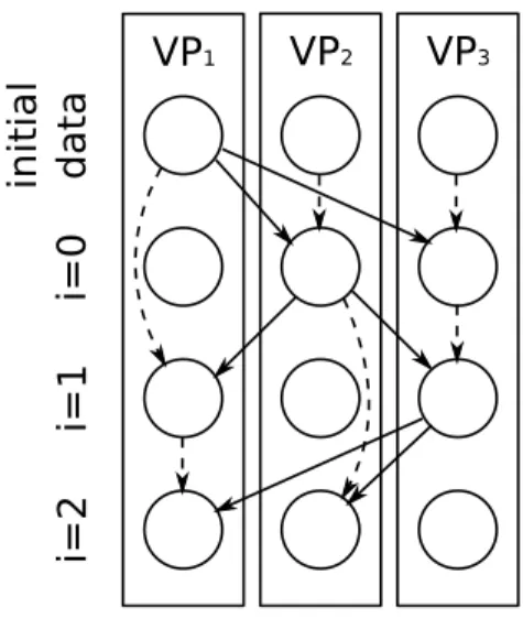
Figure 1.1: Sample execution of application with compile time support Our dynamic support needs the definition of virtual processors divided in steps, and needs to know about the dependencies between the steps. It will use these informations to conceptually model a graph of the dependencies, as figure1.2illustrates, in order to dynamically schedule the steps of the virtual

(10)

9

processors to the processing units.

initial dat a i=0 i=1 i=2 VP1 VP2 VP3

Figure 1.2: The dependency graph managed by our support

In order to achieve good results we must take into account that usually applications will be defined with a very large number of virtual processors (in the order of thousands, usually), divided in a larger number of steps each of which will execute little computation. A dynamic support will then need to manage the informations it has available in an efficient way, both in space and time.

Related works

At the state of the art, most data-parallel applications are statically defined. In the last few years research in this field focused mostly on static supports for stencil: compilers for stencil became popular, they take a sequential compu-tation in input, derive the stencil for the compucompu-tation and generate a parallel application. The virtual processors of the generated parallel application are usually statically partitioned [26, 8, 19].

This approach has anyway one major disadvantage: statically partitioned applications cannot be able to adapt to the actual execution instance. They will not be able to respond to situations that may be encountered at runtime

(11)

10

only. A typical scenario for which a static support would give bad results is an unbalanced computation. If one or more workers take more time than the others to run their job, the application completion time will equal that of the slowest worker, and the application efficiency will fall.

This work is the continuation of other works carried on by the Parallel Ar-chitecture Group of the Department of Computer Science of the University of Pisa: Salvatore Di Girolamo developed in 2011 a dynamic support for MAP data-parallel computations [10], aiming to overcome the disadvantages of static supports. Such support relied on our same models and works in a way similar to our support. The main difference is that such support does not handle stencils: does not have the concept of data dependencies, and does not need to handle them at all. Our work extends it by taking into account the stencil, thus the dependencies, offering a larger set of scheduling policies and studying the overhead in a finer way.

A big piece of our work will concern the dynamic partitioning of the virtual processors: i.e. how the virtual processors get scheduled to the real processing units. There exist a number of research projects on the dynamic scheduling of portions of code, in particular macro-data-flow [23] and task-graphs [17] seem to aid a problem quite similar to ours. We will see that our applications might be modelled in a way compatible to these two models. We can however find some main differences between our work and the several macro-data-flow and task-graph supports, like Intel Threading Building Blocks [R 20], FastFlow[3] or Cilk++[18]:

1. Our work tightly follows the virtual processor model, this will give us more information than a generic task-graph or macro-data-flow. We will see that this information may be used to approach our problem in several ways, even in ways that a graph could not easily model:

• an example is the implementation we will see in section 3.4.1.4, • the model we followed would also offer us the concept of

period-icity for the stencils and would give us information about spatial locality that, as we will discuss in section 5.1.2, could be used to

(12)

11

further optimize the support for some applications.

2. Our support is meant to work with a large number of virtual processors

made of a large number of steps. As we will see in section 3.3.1, a

support not optimized for this scenario would require too much memory and would introduce a quite large overhead. Most supports for macro-data-flow and task-graph have not our requirements and aim to offer optimizations that would be inapplicable or useless to our case.

Structure of this work

This document deals with the mentioned topics and its structure is the fol-lowing:

1. Chapter2 presents the model we are referring to, briefly introducing a taxonomy for the data-parallel computations we are interested in, and the terminology we will use.

2. Chapter 3 shows our support, its rationale and its requirements into

details, the rationale for the choice we did, its interface and its imple-mentation details.

3. Chapter4presents some applications we developed in order to test the support and shows the results of our support, compared to different im-plementations of the same computations and the overhead introduced by our support into details.

4. Chapter 5 will draw the conclusions about the work done, and will

(13)

CHAPTER

2

Programming model for data-parallel

applications

2.1 Data-parallel applications

As described in [27], a data-parallel computation is characterized by parti-tioning of (large) data structures and by function replication.

Data-parallelism is a very powerful and flexible paradigm, that can be ex-ploited in several forms according to the strategy of input data partitioning and replication, to the strategy of output data collection and presentation, and to the organization of workers (independent or interacting), though this flexibility is inevitably paid with a more complex realization of programs and of programming tools. The knowledge of the sequential computation form is necessary, both for functions and for data, and this is the main reason for the parallel program design complexity. Besides service time and completion time, latency and memory capacity are optimized compared to stream par-allel paradigms, though a potential load unbalance could exist.

As a generic example, let us consider a data-parallel computation operating on a bi-dimensional array A[M][M]. Assume that A is partitioned by square

blocks among N workers, with G = M2/N partition size. All workers apply

(14)

2.2. Virtual Processors 13

The simplest data-parallel computation is the so-called map, in which the workers are fully independent, i.e. each of them operates on its own local data only, without any cooperation with the other workers during the execution of f .

More complex, yet powerful, computations are characterized by workers that operate in parallel and cooperate (through data exchanges): this is because data dependences are imposed by the computation semantics. In this case we speak about stencil-based computations, where a stencil is a data dependence pattern implemented by inter-worker communications. The form of a stencil may be:

• statically predictable, or dynamically exploited according to the current data values,

• in the static case, the stencil may be fixed throughout the computation, or variable from a computation step to the next one (however, it is statically predictable which stencil will occur at each step).

For our work we’ll focus on stencil-based data-parallel computations.

2.2 Virtual Processors

The complexity in data parallel program design can be eased through a sys-tematic and formal approach which, starting from the sequential computa-tion, is able to derive the basic characteristics of one or more equivalent data parallel computations. The main characteristics to be recognized are:

1. how to distribute input data (partitioning and possibly replication), and how to collects output data,

2. how to understand that a map solution is possible,

3. how to understand that a stencil-based solution is possible, and, in this case, how to understand the stencil form.

(15)

2.2. Virtual Processors 14

Of course, according to our methodology, the answers to such questions must be accompanied by a cost model.

We adopt the so-called Virtual Processors approach to data parallel program design, as described in [27], consisting of two phases:

1. according to the structure of the sequential computation, we derive an abstract representation of the equivalent data parallel computation, which is characterized by the maximum theoretical parallelism compat-ible with the computation semantics. The modules of this abstract ver-sion are called (for historical reasons) Virtual Processors. Data are par-titioned among the virtual processors according to the program seman-tics. During the first phase, we are not concerned with the efficiency of the virtual processors computation: in the majority of cases, the parallelism exploited in the virtual processor version is (much) higher than the actually optimal one. However, the goal of the virtual proces-sor version is only to capture the essential features of the data parallel computation (characteristics 1, 2, 3 above). Because it is a maximally parallel version, often the grain size of data partitions is the minimum one, but this is not necessarily true in all cases (however, in general the virtual processor grain is (much) smaller than the actual one);

2. we map the virtual processor computation onto the actual version with coarser grain worker modules and coarser grain data partitions. This executable, process-level program is parametric in the parallelism de-gree n. In order to effectively execute the program, the dede-gree of par-allelism must be chosen at loading time, according to the resources that are allocated. The paradigm cost model is fully exploited dur-ing this second phase, both for derivdur-ing the parametric version and for characterizing the resource allocation strategy.

(16)

2.3. Owner computes rule 15

2.3 Owner computes rule

The virtual processors will need to respect the owner computes rule.

The owner computes rule is based on the concept of data ownership. Each module gets the ownership of the input distributed data, i.e. it is the only one that can modify those data. The owned elements are always up-to-date and need no synchronization before being accessed by the process. Usually the rule is expressed with respect to assignment statements that defines updates of variables in a program: the module that owns the left-hand side element is in charge of performing the calculation. Therefore the owner module is the only one that can update its owned data and moreover is responsible for performing all the operations on them. In case those operations required non-owned data, communications between processes are necessary.

In a local environment cooperation model, this rule is quite “natural”. Non-owned variables are non-local variables, therefore, if needed for the compu-tation, they must be acquired from the respective virtual processors. For example, in a message-passing environment, at each step every VP, encapsu-lating x, sends x to those VPs which need x during such step.

In a global environment cooperation model, which is the one we will focus our work on, resources are shared, and in order to enforce this rule data may need to be duplicated and processes must explicitly synchronize.

2.4 Example

Let us consider the sequential computation shown in listing 2.1:

1 int A[M ]

2 ∀i i n 0..M − 1:

3 ∀j i n 0..M − 1:

4 A[j] = f (A[i], A[j])

Listing 2.1: Sequential computation example

According to the Virtual Processors approach, we are able to recognize a vec-tor of M virtual processors, V P [M ], each one encapsulating a single element

(17)

2.4. Example 16

A[i], thus achieving O(M ) completion time instead of O(M2_{). We can say}

that “parallelism is applied to j”. Listing 2.2 shows in fact how a VP would look like.

1 V P [j]:

2 ∀i i n 0..M − 1:

3 A[j] = f (A[i], A[j])

Listing 2.2: Virtual Processor for the example computation

Moreover, according to the owner computes rule, at the beginning of each step VPs must interact to implement a static stencil, which is variable at each sequential step according to the j value. Figure2.1exemplify the stencil form for M = 3 and i = 0.

VP1 VP2 VP3

(18)

CHAPTER

3

Support for stencil data-parallel applications

In this chapter we will see how a support for applications modelled according to the virtual processor approach would look like and work.

3.1 Dependency graph

As we could see from the example in section2.4, a virtual processor may need to access data owned by other virtual processors a number of times during its execution.

We could imagine that each virtual processor is made of a sequence of steps. At each step a virtual processor would:

1. retrieve data of other virtual processors, 2. run some computation,

3. update its own data.

This modelling of a virtual processor usually comes quite “natural”, since most virtual processors are described with a loop that at each iteration exe-cutes the operations 1, 2 and 3 in order.

We can see that the data dependencies concern the steps of a virtual proces-sor, more than the virtual processors themselves.

(19)

3.1. Dependency graph 18

We can think of completely unfolding the virtual processors of an application (in case they are described with a loop or some other control flow statements) and see the unfolded stencil, i.e. a plain sequence of steps, as a directed graph of dependencies between the VPs at any step: each node is a pair (vp, step) that represents the step step of virtual processor vp, and each directed edge represents the data dependency between two VPs at the given steps.

Fig-ure 3.1 shows the dependency graph of the example computation presented

in section 2.4. initial dat a i=0 i=1 i=2 VP1 VP2 VP3

Figure 3.1: Dependency graph for computation in listing 2.2, with M = 3

This dependency graph is also naturally reconductible to the dataflow model [9].

One thing that we know from the dataflows, as described in [1], is that in order to handle a generic stencil, it’s not enough to have information about the dependencies of each whole VP, instead we need to have information about each step of each VP. The example stencil illustrated in figure 3.2 can help us understand this: the data dependencies from the first two virtual processors toward the third one may be satisfied in any order. A single information about the status of the dependencies of the third VP (for example a counter) wouldn’t be enough in a computation like this one to understand whether the dependencies for the second steps are met. This issue will be

(20)

3.2. Static and dynamic supports 19

seen in any dynamic stencil and in many static ones.

VP

1

VP

2

VP

3

Figure 3.2: Dependency graph for an example computation

We will often take advantage of the graph terminology while talking about our support. In particular we will talk about entering and exiting depen-dencies, which are the edges entering or exiting a node in our dependency graph:

1. the entering dependencies for a VP at a given step are the pairs (vp, step) toward which our VP depends,

2. analogously the exiting dependencies for a VP at a given step are the pairs (vp, step) that depends on our VP.

Of course for every data dependency there exists an exiting dependency for a step of a virtual processor and an entering dependency for a step of a different virtual processor.

3.2 Static and dynamic supports

A support for an application modelled according to the virtual processors approach may either be static or dynamic:

(21)

3.3. Dynamic support overview 20

• a static support would statically assign the processing of each virtual processor at each step at a predetermined processing unit.

• a dynamic support would dynamically assign a virtual processor at a step at a processing unit at runtime.

3.2.1 Static support

A static support would be able to build a working application with very little, inevitable runtime overhead: only the synchronization mechanisms to ensure that the dependencies are met. On the other side it won’t be able to adapt to the actual execution scenario, being unable to respond to situations that may be encountered at runtime only.

A typical scenario for which a static support would give bad results is an un-balanced computation. If a worker takes more time than statically speculated to run a certain portion of its job, it will slow down the whole application, and the other workers will just have to wait for him.

3.2.2 Dynamic support

The motivation for a dynamic data-parallel support is that of addressing the issues of static supports. Dynamic supports will be able to overcome issues like load unbalance.

The workers of a dynamic support, however, will have to run some man-agement code, unneeded by the application, and this will result in some overhead.

3.3 Dynamic support overview

A generic dynamic support needs to handle three main components:

1. the workers: the real processing units on which virtual processors will be mapped in order to execute their steps,

(22)

3.3. Dynamic support overview 21

2. a ready virtual processor set: a set of references to the virtual processors that may be executed, i.e. whose next step dependencies are met, 3. a structure to keep track of the status of the dependencies between

virtual processors.

At the beginning, a dynamic support will put all the virtual processors into the ready set, since the first step of any virtual processor does not have any dependency.

The support will keep taking virtual processors from the ready set and as-signing them to the free workers. As soon as a virtual processor has executed one of its steps, the worker it was assigned to releases it becoming free again, and the support will handle the exiting dependencies of the executed step, updating the corresponding entering dependencies of other virtual proces-sors; when the support notices that all the entering dependencies for the first unprocessed step of a virtual processor are met, the virtual processor will be added back to the ready set.

We will say that a worker fetches a virtual processor, when the support takes a virtual processor from the ready set and assigns it to a worker, and that a worker finalizes a (step of a) virtual processor when a virtual processor assigned to a worker finishes to execute its step, the worker releases it and the support updates the dependencies.

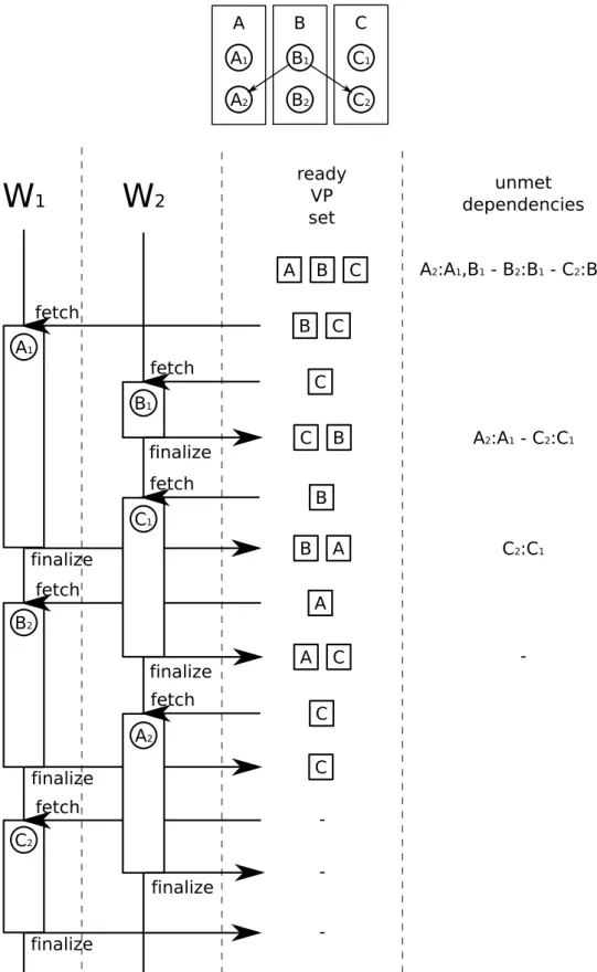
Figure 3.3 graphically shows the dependency graph for an example

applica-tion and a possible execuapplica-tion instance of a dynamic support handling the application. Note that in the image, the unmet dependencies for the steps of our VPs will also contain the preceding steps of the same VP; these are not dependencies on data, but rather dependencies due to the sequentiality of each VP.

(23)

3.3. Dynamic support overview 22 A B C

W

1

W

2 ready VP set unmet dependencies A1 fetch A2:A1,B1 - B2:B1 - C2:B1,C1 finalize fetch finalize B1 A2:A1 - C2:C1 fetch C1 C2:C1 fetch B2 finalize -finalize fetch A2 fetch finalize C2 finalize -B C C C B B A B A A C C C C C1 C2 B B2 B1 A A1 A2

(24)

3.4. Our dynamic support 23

3.3.1 Problem characterization

A runtime support should do anything possible in order to try achieving performances similar to a static implementation of a balanced data-parallel application. We must consider that our workers usually will have fetch a large number of virtual processors running small steps (in the example application

shown in section 2.4 we have M virtual processors of M steps each, for a

total of M2 _{fetching operations each of which just computes a single f ), and} this will imply a few risks:

• The cost of fetching a virtual processor might be too high compared to the actual computation cost of one of its steps.

• The memory used by the support’s data structures could be quite large, even order of magnitudes larger than the input data, given the quantity of information available.

3.4 Our dynamic support

A generic run-time support won’t probably be able to behave in an optimal way for every case; our job will be that of analysing costs and possible op-timized implementations of our support on SPM machines, for both generic cases and then for some common stencil schemas.

We chose to divide our problem in two:

• handling the dependencies, representing the dependency graph in a way efficient in space and in access time,

• fetching the virtual processors.

3.4.1 Dependency handling

3.4.1.1 Generic dataflow implementation

The complete graph of dependencies discussed so far is an abstract repre-sentation of a generic data-parallel application. It should provide all the

(25)

information a support may need in order to handle any application. Such information may be stored in memory in a variety of ways, and a number of algorithms could operate on it.

The most generic implementation is that of faithfully modelling our graph. We could implement a directed graph in memory: each virtual processor may be represented as an array of its steps; each step could be represented as a structure containing a list of its entering dependencies and another one for its exiting dependencies. The dependencies, in turn, could be implemented as a pointer to a step of virtual processors. Figure 3.4 shows the structure used to represent a virtual processor with this implementation.

VP

s[0] : step s[1] : step s[2] : step s[3] : step

step

din : deps dout: deps

deps

d[0] : step* d[1] : step* d[2] : step* d[3] : step*

Figure 3.4: Dependency graph faithful implementation

With such representation, upon completing the computation of a virtual processor at a given step, the support could access the depending steps and remove from their entering dependency list the pointer toward the completed step; upon the emptying of the entering dependency list of a step of a virtual processor, such virtual processor would be put into the ready virtual proces-sor set.

This implementation is the most trivial one, and it’s obviously a naive one: each virtual processor would waste too much memory to be represented and also the algorithms would take a lot of processing time in order to traverse the sparse graph and modify the lists of dependencies.

(26)

3.4.1.2 Matrix representation of a generic implementation

A way to optimize the generic implementation described in section 3.4.1.1

would be that of representing the graph of dependencies in a more compact way.

In most cases it’s possible to compute in constant time the entering and exiting dependencies of every step of every virtual processor, without needing to store extra data in memory for it. For example the two functions 3.1 and

3.2 define respectively the entering end exiting dependencies for the steps of the virtual processors of the example shown in section 2.4:

depsin(vp, step) =  



{ (step, step − 1) } if step 6= vp

− otherwise

(3.1)

depsout(vp, step) =  



{ (i, step + 1) | i 6= step } if step = vp

− otherwise

(3.2)

In this case it’s sufficient to only keep in memory a counter of the unmet dependencies for each step of each virtual processor. The initial value of each counter is found through the depsin function, and every time a virtual processor executes a step, the support decrements the unmet dependencies counter of the depending steps, that are found through the depsout function. When the unmet dependencies counter reaches 0 for a virtual processor at its next step, such virtual processor gets put into the ready set.

A matrix of counters is the only structure this support implementation would

need. Figure 3.5 shows the dependency matrix at the beginning of the

(27)

VP

step

0 1 2 0 1 2 1 1 0 1 0 1 0 1 1

Figure 3.5: Dependency matrix

This solution, compared to the one shown in section 3.4.1.1, takes a lot less memory: we can completely drop the list of entering and exiting dependencies (i.e. pointers to other steps) saving a lot of space. The overhead to finalize a step of a virtual processor should be very small as well.

3.4.1.3 Compressed matrix representation: frontier

It is possible to compress the dependency matrix described in section 3.4.1.2. We know in fact that we we will only need to count the number of unmet de-pendencies for the steps which have at least one met dependency but haven’t been executed yet, since we don’t need the counter of unmet dependencies for already executed steps, and the initial number of dependencies may be dynamically computed when needed for any step through the function depsin. These counters may be stored in a dynamic list, which we will refer to as frontier.

For the application taken as example in section 2.4, the frontier will never be used, since there are no steps for any virtual processor that depend on more than just a single virtual processor; that’s just a case however, for most other applications the frontier will be used, and for some particular applica-tions the frontier could contain a number of elements of the same order of magnitude of the total number of steps of any virtual processor.

It is not possible to statically associate the step of a virtual processor (vp, step) to its index in the frontier, since the frontier is dynamic. We will rather have to search for the step in the frontier, thus using a dictionary or a hash table (associating the pair (vp, step) to the counter for such step) to implement

(28)

the frontier would allow us to binary-search into the frontier.

3.4.1.4 Map with barrier

A completely different approach to face our problem could be implementing our support using a map with a barrier at each step. In order to use this support implementation, the virtual processors will need to be defined in a way such that a step of a virtual processor will only have data dependencies toward virtual processors at a previous step. This property is anyway nat-urally respected by most applications, and in particular by any application we ever met during our work.

If we only have dependencies from the step of a virtual processor to pre-ceding steps of other virtual processors, we know that once all the virtual processors have executed their i-th step, they all can execute their step i + 1, implicitly knowing that their dependencies are met. This support will fetch the virtual processors to the workers in a sequential way, and will wait for the synchronization of all workers before starting a new step.

This implementation of our support is more lightweight than the others, since we don’t need to store information about dependencies, and workers just fetch virtual processors sequentially, saving a lot of space and having lighter support functions. This support, also, doesn’t need the two functions depsin and depsout thus could be utilized as a quick solution for applications whose dependency graph is difficult to be determined.

This support however only offers parallelism among virtual processors at the same step, this could introduce some unbalance.

Figure3.6 shows how the virtual processors of a possible example application with an unknown stencil could be fetched by some workers.

(29)

3.4. Our dynamic support 28 C C1 C2 B B2 B1 A A1 A2 ?

W

1

W

2

W

3 step 0 A1 B1 C1 step 1 A2 B2 C2

Figure 3.6: Map with barrier implementation overview

3.4.2 Fetching virtual processors

All the computational overhead introduced by our support is into the func-tions to fetch and to finalize a virtual processor: these are the only two functions of the support that will be called during the computation.

We studied a number of strategies to speed up these two functions and to schedule jobs in a smart way.

(30)

3.4.2.1 Critical sections

The functions to fetch and to finalize a virtual processor needs to manipulate some shared data structures, in particular the finalizing function will need to update the graph of dependencies, and both the fetching and the finalizing functions will need to update the set of ready virtual processors.

In order to access shared structures avoiding race conditions we could either use atomic operations or define some critical sections that only one worker may access at a time. Several strategies have been studied and tested out.

Single critical section The simplest way to avoid race conditions is just

marking the whole fetching and finalizing functions as critical, using a single mutex to lock all the shared data structures.

Two critical sections An improvement over the previous solution would

be that of dividing our support functions in two critical sections: one for each data structure. The fetching function will just need to access the set of ready jobs in a mutually exclusive way, thus acquiring a single mutex, while the finalizing function will access at the beginning the dependency graph and then the ready list, thus it could acquire and release two mutexes during its execution.

A critical section plus one per VP An even more fine grained solution

could be that of dividing the access to the dependency graphs in many critical sections. Usually the function to finalize a step of a virtual processor will need to mark a lot of dependencies as satisfied, thus it could acquire a mutex only for one or a few of them at a time.

Single critical section and atomic operation Many architectures

(in-cluding the Intel computers we will run our simulations on) provide some as-sembly instructions to atomically compute simple operations, like subtraction or decrementing. Some implementations of the dependency graph (in par-ticular the implementation using a matrix) could exploit these instructions

(31)

to update the dependency counters without needing to acquire an exclusive access on the graph.

3.4.2.2 Fetching several virtual processors at once

As we have seen in section 3.4.2.1, the fetching and finalizing functions need some mechanisms to ensure thread safe access to our support data structures. These mechanisms have an overhead on their own, that in some cases could be quite large. In particular if we have a large number of workers that fetch a lot of times the virtual processors executing little computation, our fetching and finalizing functions will be accessed very often, and the cost due to the synchronization mechanisms would be large.

A possible strategy to lighten this overhead could be that of letting the workers fetch and finalize multiple virtual processors per time. This way a worker will spend more time processing virtual processors between any fetching and finalizing operation, and the overall number of critical sections entered will decrease.

A static number of virtual processors fetched per time could be harmful, since it could lead to the unbalance issues we are fighting in the first place, thus a smarter strategy should be chosen. We defined a couple of strategies to specify to the support how many virtual processors fetching per time. These strategies depend on an application-dependent value and on two variable values of the support that may change over time:

• R, the number of ready virtual processors, the size of the ready VP set, • N, the number of workers.

Strategy 1: fetching up to Q VPs at once One of the simplest way to

approach this problem could be that of fetching min(Q,_NR) virtual processors at once. Q is an integer specified by the application.

Strategy 2: application balancedness coefficient A more

sophisti-cated and more generic strategy could be that of fetching a subset of the ready virtual processors depending on how balanced the application is.

(32)

P , the application balancedness coefficient, represents how balanced an ap-plication is, and is a parameter specified by the apap-plication. It should be set to 1 for a highly balanced application, and to lower values for unbalanced applications. If P is set to a value smaller than its optimal, what happens is that each worker fetches little virtual processors per time and runs the fetching and finalizing functions more often that it would need to. If P is set to a value larger than its optimal, it may happen than an unlucky worker Wu fetches many heavyweight virtual processors, and before it is done process-ing such VPs the other workers are already finished; this would in practice introduce the same unbalance issues a dynamic support is trying to combat. It’s possible to find a lower bound for P , Plb such that even at the worst case the computation will not become unbalanced. Let’s suppose that we know the minimal and the maximum possible duration for the quickest and the slowest steps of our virtual processors, let’s call them Tmin and Tmax respec-tively. Any worker will regularly fetch P R

N virtual processors at once, and the worst case computation, i.e. the one that would unbalance the workers the most, is the computation in which:

• no virtual processors will be added to the ready VP set, i.e. our compu-tation was just a map; if we in fact take the same compucompu-tation, modified so that some virtual processors are added back to the ready set dur-ing the computation, the workers would be less unbalanced, since some of the workers that are finished would fetch the newly added virtual processors.

• The virtual processors fetched by Wuall take Tmaxtime to execute their step, while the other workers only fetch lightweight virtual processors taking Tmin to execute their step; In other cases the difference of

com-putation between Wu and the other workers would be lower, thus the

application would be less unbalanced.

In this scenario Wu would fetch P_NR virtual processors, and will have a total execution time of TmaxP_NR. All the other N − 1 workers would fetch all

(33)

each worker would be Tmin(R−PR_N)

N −1 . Our Plb will equal the duration of the

computation of Wu with that of any other worker: Plb =

N Tq

(N − 1)Tmax+ Tmin

Any value of P bigger than Plb would result in a possible unbalance for the worst case, while for any value smaller than Plb, any worker (even our unlucky one) would complete the processing of its virtual processors while there still are some VPs to be computed, thus we would do more fetching and finalizing operations than needed.

In the special case where Tmin = Tmax, all the virtual processors take the same computation time, Plb will be 1 and any worker will fetch exactly _NR virtual processors.

Of course this is a lower bound for the very worst case, quite unlikely to

happen. A value somewhere between Plb and 1 would typically be better. It

would also be possible to find better (i.e. higher) lower bounds for specific applications when knowing some properties of the dependency graph or of the virtual processor computation times.

A value for Plb not depending on N would be T_Tq_s. In fact Plb ≥ T_Tq_s and for N → ∞, Plb → T_Tq_s.

3.4.2.3 Null steps

Some computations may be naturally defined in a way that some steps for some virtual processors (or even whole virtual processors) don’t need to do anything at all.

Applications with this property wouldn’t perform at their best with some of our support implementations, they would introduce a higher overhead, since the number of fetching and finalizing operations is higher than the total number of steps, and would limit the number of virtual processors fetched at once when using the optimization described in section 3.4.2.2.

It would be possible to avoid the execution of null steps without the needing of modifying the stencil in a simple way; the application would need to pass

(34)

to the support also the dependencies intra-VP: a dependency must be defined between vp, stepi and vp, stepj if:

1. i < j,

2. stepi and stepj are not null, i.e. the application needs both of them to be executed,

3. ∀ x : i < x < j, stepx is null, i.e. the application does not need it to be executed.

Once the virtual processors have been defined like this by the application, the support will put the virtual processors into the ready VP set as soon as one of their steps has all the dependencies met, even if it’s not the first non-executed step, and will have to pass the step index to the virtual processors when fetching them.

Figure 3.7 shows how the dependency graph for computation in section 2.4

would need to be modified to exploit this optimization.

initial dat a i=0 i=1 i=2 VP1 VP2 VP3

Figure 3.7: Dependency graph for computation in section2.4, with M = 3

All our support implementations can exploit this optimization, that will be particularly useful with some of the applications we studied and tested, as we will see in chapter 4.

(35)

3.4.3 Support interface

The application using our support must feed the latter with: 1. The virtual processors.

2. What support implementation to use.

3. A function to retrieve the entering dependencies of a step of a virtual processor. (Not needed for map with barrier implementation.)

4. A function to retrieve the exiting dependencies of a step of a virtual processor. (Not needed for map with barrier implementation.)

• The number of Virtual Processors. • The number of steps for any VP.

• The number of threads the support should spawn.

• Optionally, the application balancedness coefficient described in sec-tion 3.4.2.2.

3.4.3.1 Details

The support, written in C++, widely uses templates in order to get stati-cally optimized as much as possible. The solution representing the graph of dependencies (2.) will be a template parameter of our support.

The two functions to retrieve virtual processors (3. and 4.) should seman-tically generate a set of elements and return it. This set is often used by the support to access small bits of information only, for example the set size only. We ran some tests and noticed that the compiler isn’t able to optimize enough a function that generates a set of elements and returns it, since the management of a dynamic set would require many operations with side ef-fects, like functions to dynamically allocate more memory. For this reason we chose a smarter solution: passing a callback (i.e. a pointer to a function) to the application function; this callback should be called for any element

(36)

the application function should add to the set; the callback function, pro-vided by the support, may build the whole set, if that’s what the support needs, or just increment a counter, if the support only wants to know about the size of the set of elements generated by the application functions. As our results have shown, the compiler will be able to optimize this a lot, the compiled function will be equivalent to the naive version when the support needs the whole set, or will be a lot more lightweight when the support needs only partial information. In many common cases, like that of counting how many elements the application function generates, the compiler will be even able to flatten the whole functions and just replace the calls with a simple mathematical expression.

The other parameters the application must feed the support with are just numeric values that needs to be passed to the support class constructor.

3.4.4 Tools to develop an efficient runtime support

In order to develop an efficient stencil support we will use low level tools which will keep the overhead to a minimum. In particular we will use:

• POSIX threads (pthreads) offered by Linux kernel and glibc to imple-ment the workers [24]. We don’t have lower level alternatives. Another approach would that of using processes; this would allow the applica-tion to work on distributed memory systems, but will also imply some more overhead when compared to threads.

• Shared memory to share data amongst the several workers. This feature is automatically provided by POSIX threads. During the testing phase we will also use POSIX shared memory segments to share large data between non-cooperating applications instead of writing and reading it [22].

• Custom synchronization mechanisms: spin locks and custom condition variables built above the spin locks [5]. These would have less overhead than POSIX synchronization mechanisms like mutexes, and will force

(37)

active waiting, which is a good thing for a performance critical appli-cation where overhead and time wasted in synchronization should be reduced to a minimum.

• Machine-dependent cycle counters code to take times in order to study into details the costs of any piece of our support. We will use some functions and macros offered by Matteo Frigo [12] relying, for intel processors, on the rdtsc instruction.

• Atomic operations will be used to atomically access some data struc-tures as a possible alternative to mutual exclusion mechanisms [15]. The support will be implemented in C++11 [14], exploiting as much as possi-ble static time features like templates, and avoiding slow runtime functional-ities like dynamic memory allocation. We will also use some C++ Standard Template Library and Boost Library data structure and functionalities [7], after ensuring they respect our strict performance requirements.

3.4.5 Implementation

The support has been logically divided in three main components:

• DPSup: it’s the only module of the support exposed to the applica-tion. It represents the support itself, its interface is the one visible to the application. It will handle the other two components and their interaction.

• AbstractProcessor, abbreviated as AP: it’s the module representing one worker.

• JobFactory, abbreviated as JF: it’s the module representing the graph of dependencies and the ready VP set.

(38)

DPSup

JF

AP

Figure 3.8: Support abstract view

3.4.5.1 DPSup

DPSup implementation is quite simple: upon construction it instantiates the AbstractProcessors, the JobFactory and waits for its run function to be called. The run function waits that all the AbstractProcessors are ready, starts them all and waits for their termination. This semantics is implemented using a pthread barrier.

3.4.5.2 AbstractProcessor

AbstractProcessor basically spawns a pthread in its constructor, destroys it in the destructor and for its lifetime just executes the simple loop whose pseudo-code is shown in listing 3.1:

1 APi: 2 while not f i n i s h e d : 3 vps = f e t c h () 4 f o r vp i n vps : 5 vp . r u n S t e p ( ) 6 f i n a l i z e ( vps )

Listing 3.1: AbstractProcessor main loop

3.4.5.3 JobFactory

JobFactory is the module handling the virtual processors and the graph of dependencies. We offered the four implementations of JobFactory discussed in

(39)

section3.4.1, but other implementations may be provided by the application or third part libraries.

The Jobfactory module must expose a function to fetch and to finalize a set of virtual processors and to check whether the parallel computation is completed.

Dependency matrix implementation The implementation for

JobFac-tory using a dependency matrix discussed in section 3.4.1.2 has several vari-ants, one for each kind of fetching strategy. We are going to consider a simplified version without critical sections.

Upon construction, this JobFactory creates the matrix of counters: each ele-ment (i, j) represents the number of unmet dependencies for the j-th step of the i-th VP. At the beginning all the virtual processors are inserted into the ready VP set.

The fetching function, whose pseudo-code is listed in listing 3.2, has just to take some elements from the ready VP set.

1 f e t c h :

2 while not f i n i s h e d and r e a d y V P S e t empty :

3 w a i t on c o n d i t i o n v a r i a b l e C

4 f o r i i n {0..PR_N}:

5 f e t c h r e a d y V P S e t . t a k e ()

Listing 3.2: JobFactory with depency matrix fetching function

The finalizing function is a little more complex, since it needs to handle the dependency matrix. It will decrement the unmet dependencies for the steps depending on the one we’re finalizing, and will add these virtual processors to the ready set if all their dependencies are met. It’s pseudo-code is shown in listing 3.3. 1 f i n a l i z e ( vp , s t e p ) : 2 f o r t i n a p p l i c a t i o n . e x i t i n g D e p e n d e n c i e s ( vp , step ) : 3 d e p e n d e n c y M a t r i x [ t ] -= 1 4 i f d e p e n d e n c y M a t r i x [ t ] == 0: 5 r e a d y V P S e t . add ( t )

(40)

6 w a k e up a w o r k e r s l e e p i n g on C

7 i f f i n i s h e d :

8 w a k e up all w o r k e r s s l e e p i n g on C

Listing 3.3: JobFactory with depency matrix finalizing function

Dependency frontier implementation Also the implementation using

the frontier discussed in section 3.4.1.3has several variants, and also in this case we’ll just take a simplified version free of critical sections.

The frontier will be empty at the beginning, and as usual this support will just put all the virtual processors into the ready. The fetching function is the same of the dependency matrix implementation shown in listing 3.2. The finalizing function is instead different: here we won’t handle dependen-cies through the matrix, but will use the frontier instead. When the unmet dependencies of a step must be decreased, we first check whether the step has a single entering dependency: in such case we just add it to the ready set, otherwise we check whether the step is already present into the frontier: if it’s not, it gets added; if it was instead present, its number of unmet depen-dencies gets decremented and if it becomes 0 the step gets removed from the frontier and the virtual processor put into the ready set. The pseudo-code for the finalizing function is shown in listing 3.4.

1 f i n a l i z e ( vp , s t e p ) : 2 f o r t i n a p p l i c a t i o n . e x i t i n g D e p e n d e n c i e s ( vp , step ) : 3 i f a p p l i c a t i o n . e n t e r i n g D e p e n d e n c i e s ( t ) . c o u n t == 1: 4 r e a d y V P S e t . add ( t ) 5 e l s e : 6 i f not f r o n t i e r . c o n t a i n s ( t ) : 7 f r o n t i e r [ t ] = app . e n t e r i n g D e p s ( t ) . c o u n t () -1 8 e l s e : 9 f r o n t i e r [ t ] -= 1 10 i f f r o n t i e r [ t ] == 0: 11 r e a d y V P S e t . add ( t ) 12 f r o n t i e r . r e m o v e ( t ) 13 w a k e up a w o r k e r s l e e p i n g on C

(41)

14 i f f i n i s h e d :

15 w a k e up all w o r k e r s s l e e p i n g on C

Listing 3.4: JobFactory with frontier finalizing function

Map with barrier implementation The implementation using the map

with barrier discussed in section 3.4.1.4 needs to use a barrier. We tried by using both the pthread barrier and a custom barrier implemented using our spin locks.

The finalizing function in this case doesn’t need to do anything at all. The fetching function instead needs to take a bunch of virtual processors at the given step in a mutually exclusive way. If a worker cannot find any virtual processor it should stop on a barrier, the last worker stopping on it will have to reset the data structures to handle the next step before opening the barrier. The pseudo-code of the fetching function is shown in listing 3.5.

1 n e x t V P = 0 // n e x t VP to be f e t c h e d 2 s t e p = 0 // s t e p we are w o r k i n g on 3 f e t c h : 4 i f n e x t V P == vps : // no m o r e VPs at t h i s s t e p 5 i f b a r r i e r . c o u n t < workers -1: 6 // s o m e w o r k e r s are s t i l l p r o c e s s i n g 7 w a i t on b a r r i e r 8 e l s e :

9 // t h i s i s the last worker

10 s t e p += 1 11 n e x t V P = 0 12 o p e n b a r r i e r 13 14 i f s t e p = s t e p s : // all s t e p s p r o c e s s e d 15 return 16 17 f o r i i n {0..vps_N }: 18 f e t c h n e x t V P

(42)

19 n e x t V P += 1

(43)

CHAPTER

4

Tests and benchmarks

In order to test the support correctness and to study its overhead and its performance we took the parallel version of some existing data-parallel ap-plication and ported it on our support.

4.1 Testing environment

Our applications have been built using GCC 4.6.2 with optimization options

“-O3 -finline-functions -DNDEBUG” [11].

We ran our tests on two SMP machines available at the department of com-puter science: Titanic and Andromeda.

For any taken time, we ran each test a number of times and then computed the average value.

4.1.1 Titanic

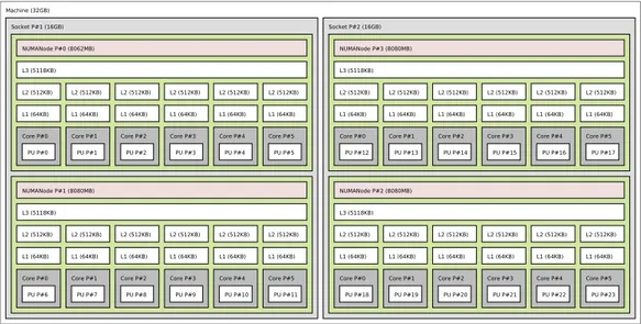
Titanic, available at the address titanic.di.unipi.it ships 24 AMD OpteronTM Processor 6176 processors, at 2300 MHz each. Each processor has 64KB of L1 cache and 512KB of L2 cache. Four groups of six processors share a single L3 cache of 5MB. Titanic has two sockets, each of which contains two of the four groups of six processors described [4].

(44)

4.1. Testing environment 43

i-th worker of our support is mapped on the i-th core of Titanic. Figure 4.1 shows in details what described so far.

Machine (32GB) Socket P#1 (16GB) NUMANode P#0 (8062MB) L3 (5118KB) L2 (512KB) L1 (64KB) Core P#0 PU P#0 L2 (512KB) L1 (64KB) Core P#1 PU P#1 L2 (512KB) L1 (64KB) Core P#2 PU P#2 L2 (512KB) L1 (64KB) Core P#3 PU P#3 L2 (512KB) L1 (64KB) Core P#4 PU P#4 L2 (512KB) L1 (64KB) Core P#5 PU P#5 NUMANode P#1 (8080MB) L3 (5118KB) L2 (512KB) L1 (64KB) Core P#0 PU P#6 L2 (512KB) L1 (64KB) Core P#1 PU P#7 L2 (512KB) L1 (64KB) Core P#2 PU P#8 L2 (512KB) L1 (64KB) Core P#3 PU P#9 L2 (512KB) L1 (64KB) Core P#4 PU P#10 L2 (512KB) L1 (64KB) Core P#5 PU P#11 Socket P#2 (16GB) NUMANode P#3 (8080MB) L3 (5118KB) L2 (512KB) L1 (64KB) Core P#0 PU P#12 L2 (512KB) L1 (64KB) Core P#1 PU P#13 L2 (512KB) L1 (64KB) Core P#2 PU P#14 L2 (512KB) L1 (64KB) Core P#3 PU P#15 L2 (512KB) L1 (64KB) Core P#4 PU P#16 L2 (512KB) L1 (64KB) Core P#5 PU P#17 NUMANode P#2 (8080MB) L3 (5118KB) L2 (512KB) L1 (64KB) Core P#0 PU P#18 L2 (512KB) L1 (64KB) Core P#1 PU P#19 L2 (512KB) L1 (64KB) Core P#2 PU P#20 L2 (512KB) L1 (64KB) Core P#3 PU P#21 L2 (512KB) L1 (64KB) Core P#4 PU P#22 L2 (512KB) L1 (64KB) Core P#5 PU P#23

Figure 4.1: Titanic topology

4.1.2 Andromeda

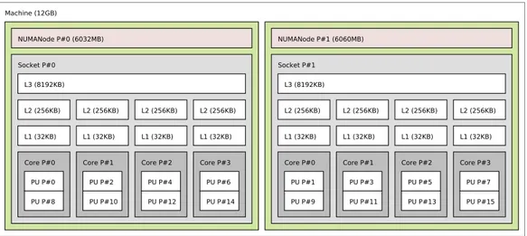
Andromeda, available at the address andromeda.di.unipi.it ships 16 Intel R

Xeon CPU E5520 processors, at 2270 MHz each. Multithreading is en-R

abled on Andromeda: each pair of processors resides on a single physical unit. Each physical unit has 32KB of L1 cache and 256KB of L2 cache. Two groups of four physical units belong each to a different socket and share a single L3 cache of 8MB [13].

We chose to map each worker on a different physical unit, without exploiting multithreading, since it would give unpredictable results and a scenario like ours, where workers use active waiting, is not a good one for multithreading. We wish to exploit cache locality as much as possible also on L3 cache, so we mapped each of our workers (up to 8) on the cores 0, 2, 4, 6, 1, 3, 5, 7 in that order.

(45)

4.2. Cholesky 44 Machine (12GB) NUMANode P#0 (6032MB) Socket P#0 L3 (8192KB) L2 (256KB) L1 (32KB) Core P#0 PU P#0 PU P#8 L2 (256KB) L1 (32KB) Core P#1 PU P#2 PU P#10 L2 (256KB) L1 (32KB) Core P#2 PU P#4 PU P#12 L2 (256KB) L1 (32KB) Core P#3 PU P#6 PU P#14 NUMANode P#1 (6060MB) Socket P#1 L3 (8192KB) L2 (256KB) L1 (32KB) Core P#0 PU P#1 PU P#9 L2 (256KB) L1 (32KB) Core P#1 PU P#3 PU P#11 L2 (256KB) L1 (32KB) Core P#2 PU P#5 PU P#13 L2 (256KB) L1 (32KB) Core P#3 PU P#7 PU P#15

Figure 4.2: Andromeda topology

4.2 Cholesky

We took a data-parallel Cholesky decomposition implementation developed by the Laboratorio di Architetture Parallele e Distribuite (parallel and dis-tributed architectures laboratory) of the computer science department of the University of Pisa, and ported it on our support.

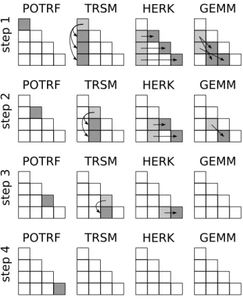
The Cholesky decomposition algorithm decomposes a Hermitian positive-definite matrix into the product of a lower triangular matrix and its conju-gate transpose. The application we took divides the matrix in some blocks and processes sequentially any block: every block is a square set of matrix cells and is assigned to a Virtual Processor. We can think of a block as a set of virtual processors operating on single cells that have been joined together with a static partitioning.

A simplified version of the pseudo-code for this block Cholesky algorithm is shown in listing 4.1. It utilizes four functions of LAPACK (Linear Algebra PACKage) and BLAS (Basic Linear Algebra Subprograms) mathematical libraries:

POTRF Computes the Cholesky factorization of a symmetric (Hermitian) positive-definite matrix.

(46)

4.2. Cholesky 45

TRSM Solves a matrix equation.

HERK Performs a rank-k update of a Hermitian matrix.

GEMM Computes a scalar-matrix-matrix product and adds the result to a scalar-matrix product.

These functions work sequentially.

1 f o r any column s:

2 // 1. POTRF - ing c e l l of c u r r e n t c o l u m n on the

3 // d i a g o n a l (s, s) 4 M [ s , s ] = P O T R F ( M [ s , s ] ) 5 // 2. TRSM - ing c e l l of c u r r e n t c o l u m n on the 6 // d i a g o n a l (s, s), on the c e l l s b e l o w (r, s) 7 f o r any row r > s: 8 // M [ r , s ] = M [ r , s ] / M [ s , s ]^ T 9 M [ r , s ] = T R S M ( M [ s , s ] , M [ r , s ] )

10 // 3. HERK - ing c e l l s of c u r r e n t c o l u m n b e l o w the

11 // d i a g o n a l (r, s), on the d i a g o n a l of t h e i r row (r, r)

12 f o r any row r > s:

13 // M [ r , r ] = M [ r , r ] - M [ r , s ] * M [ r , s ]^ T

14 M [ r , r ] = H E R K ( M [ r , s ] , M [ r , r ] )

15 // 4. GEMM - ing c e l l s of c u r r e n t c o l u m n b e l o w the

16 // d i a g o n a l , on o t h e r c e l l s b e l o w the d i a g o n a l

17 f o r any column c > s:

18 f o r any row r > c:

19 // M [ r , s ] = M [ r , s ] - M [ r , c ] * M [ s , c ]^ T

20 M [ r , s ] = G E M M ( M [ r , c ] , M [ s , c ] , M [ r , s ] )

Listing 4.1: Cholesky decompositino algorithm

Figure 4.3 represents the algorithm in action on a matrix divided in 4 × 4

blocks: darker blocks represent the ones that are written in a given phase, lighter ones represent the blocks that are read and the arrows help understand what the latter are read for.

(47)

4.2. Cholesky 46

POTRF TRSM HERK GEMM

st ep 1 st ep 4 st ep 3 st ep 2

Figure 4.3: Representation of cholesky algorithm

4.2.1 With compile time support

The original data-parallel application was written using threads. Each thread took ownership of a few rows properly chosen in order to assign the same number of blocks to any thread and thus trying to have a balanced compu-tation. The computation run by any thread is very similar to the original pseudo-code, with the only difference that each thread only iterates on the rows it has ownership of.

In order to avoid race conditions, and thus respecting the dependencies be-tween data accesses, this implementation utilized a semaphore for each block. Each semaphore is implemented using a byte set to 0 at the beginning: any thread waiting on a semaphore would actively wait for such byte to become 1. These semaphores are used to enforce the dependencies between POTRF and TRSM and between TRSM and GEMM. The other dependencies don’t

(48)

4.2. Cholesky 47

need to be explicitly expressed, since they are implicit due to the sequential-ity of a thread’s routine. We could also note that the sequentialsequential-ity of threads added also an unneeded dependency: a dependency between the HERK and the GEMM operations on a row at each step.

We may expect that this implementation using a large number of small blocks wouldn’t perform at its best, due to the overhead of the semaphores. On the contrary using a small number of large blocks, the application would proba-bly suffer of unbalance issues as discussed in [16] and as we can see from the figure4.4, showing how each thread runs its operations in a sample execution of the application using four workers and a 4 × 4 matrix.

(49)

4.2. Cholesky 48

4.2.2 Runtime support

We implemented this same algorithm using our support, just by moving the actual invocation of the mathematical functions into our virtual processors steps. Each virtual processor owns a single block, and at each step a virtual processor may execute a single mathematical operation or nothing. Since the HERK and GEMM operations are independent, they are executed at the same steps. The number of steps is thus M × 3, where M is a side

of the matrix. The stencil we managed to defined is shown in figure 4.5.

This modelling of the computation using virtual processors is compatible with all the support implementations we provided. A very large number of steps of the virtual processors we defined don’t do anything at all, thus the optimization shown in section 3.4.2.3 comes really handy.

(50)

4.2. Cholesky 49

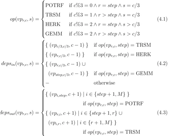
The functions defining the dependencies between steps are the following:

op(vpr,c, s) =                POTRF if c%3 = 0 ∧ r = step ∧ s = c/3 TRSM if c%3 = 1 ∧ r > step ∧ s = c/3 HERK if c%3 = 2 ∧ r = step ∧ s > c/3 GEMM if c%3 = 2 ∧ r > step ∧ s > c/3 (4.1) depsin(vpr,c, s) =                      { (vpc/3,c/3, c − 1) } if op(vpr,c, step) = TRSM { (vpr,c/3, c − 1) } if op(vpr,c, step) = HERK { (vpr,c/3, c − 1) ∪

(vpstep,c/3, c − 1) } if op(vpr,c, step) = GEMM

− otherwise (4.2) depsout(vpr,c, s) =                      { (vpi,step, c + 1) | i ∈ {step + 1, M } } if op(vpr,c, step) = POTRF { (vpr,i, c + 1) | i ∈ {step + 1, r} ∪

(vpi,r, c + 1) | i ∈ {r + 1, M } }

if op(vpr,c, step) = TRSM

(4.3)

Figure 4.6 offers a quick graphical idea of what happens with our support:

it shows how the virtual processors of a matrix of 4 × 4 blocks are scheduled to four workers in a sample execution. The runtime support implementation utilized was the one using a matrix of dependencies. It’s the same scenario previously illustrated in figure 4.4; we can see that unbalance issues are resolved.

(51)

4.2. Cholesky 50

Figure 4.6: Sample execution of application with our runtime support

4.2.3 Comparison of the different implementations

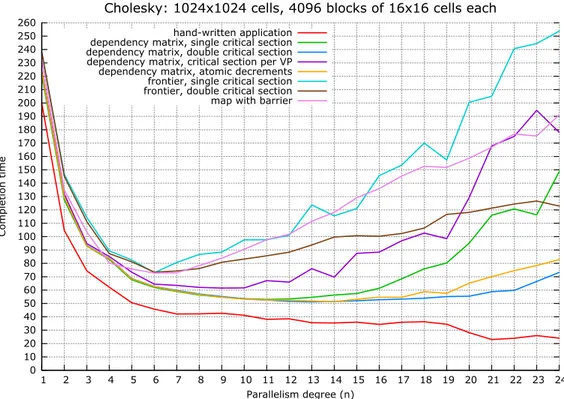
We have run thousands of tests varying the several parameters in order to compare our dynamic support implementations and the hand-written appli-cation. Here we are going to show only three of the most significant results, that let us understand best how the computation behaves and why.

The three scenarios we chose are:

1. a small matrix (1024 × 1024 cells) divided in a large number of small blocks (4096 blocks of 16 × 16 cells each),

(52)

4.2. Cholesky 51

2. a small matrix (1024 × 1024 cells) divided in a smaller number of larger blocks (256 blocks of 64 × 64 cells each),

3. a larger matrix (4096 × 4096 cells) divided in small number of large blocks (1024 blocks of 128 × 128 cells each).

In any scenario our workers fetched multiple virtual processors, as discussed in section 3.4.2.2. We used the simplest strategy fetching min(Q = 32,_NR) virtual processors at once.

4.2.4 Scenario 1: small matrix, many small blocks

This first scenario is the most critical one. It divides a quite small matrix (1024 × 1024 cells) in a large number of very small blocks (64 × 64 = 4096 blocks of 16×16 = 256 cells each). For how the virtual processors are defined, each of the 4096 virtual processors is made of 190 steps, for a total number of 778240 steps. The number of non-null virtual processor steps is 45760.

4.2.4.1 Ttitanic

Figure4.7 shows the computation completion time with respect to the

num-ber of workers of the hand-written application (in red), and of our dynamic

support implementations running on titanic. Figure 4.8 shows instead the

(53)

4.2. Cholesky 52 0 10 20 30 40 50 60 70 80 90 100 110 120 130 140 150 160 170 180 190 200 210 220 230 240 250 260 1 2 3 4 5 6 7 8 9 10 11 12 13 14 15 16 17 18 19 20 21 22 23 24 Completion time Parallelism degree (n)

Cholesky: 1024x1024 cells, 4096 blocks of 16x16 cells each

hand-written application dependency matrix, single critical section dependency matrix, double critical section dependency matrix, critical section per VP dependency matrix, atomic decrements frontier, single critical section frontier, double critical section map with barrier

Figure 4.7: Completion time of the different implementations for scenario 1 on titanic

Runtime support for stencil data-parallel applications on multicore architectures

Università di Pisa and Scuola Superiore Sant’Anna

Master Program in Computer Science and Networking

Master thesis

Runtime support for stencil

data-parallel applications on

multicore architectures

Candidate

Supervisor

Paolo Giangrandi

Prof. Marco Vanneschi

Contents

List of Figures

Listings

CHAPTER

1

Introduction

A dynamic support for stencil data-parallel applications

Related works

Structure of this work

CHAPTER

2

Programming model for data-parallel

applications

2.1

Data-parallel applications

2.2

Virtual Processors

2.3

Owner computes rule

2.4

Example

CHAPTER

3

Support for stencil data-parallel applications

3.1

Dependency graph

VP

VP

VP

3.2

Static and dynamic supports

3.2.1

Static support

3.2.2

Dynamic support

3.3

Dynamic support overview

W

W

3.3.1

Problem characterization

3.4

Our dynamic support

3.4.1

Dependency handling

VP

step

deps

VP

step

W

W

W

3.4.2

Fetching virtual processors

3.4.3

Support interface

3.4.4

Tools to develop an efficient runtime support

3.4.5

Implementation

DPSup

JF

AP

CHAPTER

4

Tests and benchmarks

4.1

Testing environment