Innovative algorithms and data structures for signal treatment applied to ISO/IEC/IEEE 21451 smart transducers

Innovative Algorithms and

Data Structures for Signal

Treatment applied to

ISO/IEC/IEEE 21451

Smart Transducers

C

:

F

A

C

:

P

.

M

LONGO

T

:

P

.

V

P

Summary

Summary... 2

Introduction ... 4

Chapter 1 Networking Measurement for an Interconnected World ... 6

1.1 The Internet of Things ... 6

1.1.1 An overview ... 6

1.1.2 Obstacles to be overcome ... 9

1.2 Smart Sensors ... 13

1.3 An example: CAN bus protocol ... 14

1.3.1 CANopen and CiA ... 19

Chapter 2 A Standard Approach for Smart Transducers ... 20

2.1 A family of standards ... 21

2.1.1 Advantages ... 25

2.2 Existing Standards ... 26

2.2.1 IEEE 1451.0 ... 26

2.2.1.1 TEDS – Transducer Electronic Data Sheet ... 27

2.2.2 IEEE 1451.1 ... 29 2.2.3 IEEE 1451.2 ... 30 2.2.4 IEEE 1451.3 ... 30 2.2.5 IEEE 1451.4 ... 32 2.2.6 IEEE 1451.5 ... 32 2.2.7 IEEE p1451.6 ... 33 2.2.8 IEEE 1451.7 ... 35

2.3 Issues regarding consistency and interoperability ... 35

Chapter 3 The ISO/IEC/IEEE 21451.001 proposal, based on a segmentation and labeling algorithm... 36

3.1 A novel approach to signal preprocessing ... 38

3.2 A real time segmentation and labeling algorithm ... 40

3.2.1 Segmentation Step ... 40

3.2.2 Labeling Step ... 44

3.3 Draft proposal for a recommended practice ... 45

3.4 First layer algorithms ... 46

3.4.1 Exponential Pattern Detection ... 46

3.4.2 Noise Detection ... 49

3.4.3 Impulsive Noise Detection ... 50

3.4.4 Sinusoidal Pattern Detection ... 52

3.4.5 Tendency Estimation ... 54

4.2.2 Noise Detection ... 74

4.2.3 Sinusoidal Pattern Detection ... 74

4.2.4 Tendency Estimation ... 75

4.2.5 Mean Estimation ... 76

Chapter 5 Applications of a RTSAL technique ... 77

5.1 Period Measurement ... 78

5.1.1 Maximum search ... 81

5.1.2 Simulation of period computation ... 84

5.1.3 Experimental results for period computation ... 94

5.1.4 A comparison with another sensor signal preprocessing techniques: compressive sampling ... 96

5.1.5 Period measurement with an ARM microcontroller .... 106

5.2 Mean estimation with RTSAL algorithm ... 107

5.3 Analysis of vibrations signals from faulty bearing ... 112

Conclusions ... 116

Acknowledgements ... 117

Introduction

Technologies and, in particular sensors, permeate more and more application sectors. From energy management, to the factories one, to houses, environments, infrastructure, and building monitoring, to healthcare and traceability systems, sensors are more and more widespread in our daily life. In the growing context of the Internet of Things capabilities to acquire magnitudes of interest, to elaborate and to communicate data is required to these technologies. These capabilities of acquisition, elaboration, and communication can be integrated on a unique device, a smart sensor, which integrates the sensible element with a simple programmable logic device, capable of managing elaboration and communication.

An efficient implementation of communication is required to these technologies, in order to better exploit the available bandwidth, minimizing energy consumption. Moreover, these devices have to be easily interchangeable (plug and play) in such a way that they could be easily usable.

Nowadays, smart sensors available on the market reveal several problems such as programming complexity, for which depth knowledge is required, and limited software porting capability.

The family of standards IEEE 1451 is written with the aim to define a set of common communication interfaces. These documents come from the Institute of Electric and Electronic Engineers (IEEE) with the aim to create a standard interface which allows devices interoperability produced from different manufacturers, but it is not concerned with problems related to bandwidth, management, elaboration and programming. For this family of standards, now under review, it is expected a further development, with the aim to renew applicable standards, and to add new layers of standardization.

The draft of the ISO/IEC/IEEE 21451.001 proposes to solve problems related to the bandwidth and the elaboration management,

shown, in the context of the Internet of Things;

 in the second chapter the actual smart sensor family of standards is shown, and their own problems are underlined;

 in the third chapter the proposed algorithm for the standardization is shown, with the related signal processing algorithms of the first and the second layer;

 in the fourth chapter RTSAL algorithm characteristics are analyzed, and a feasible implementation of the first layer algorithms on a microcontroller is shown;

 in the fifth chapter RTSAL algorithm results are shown, used for period and mean computation applications, and an application of this technique for the analysis of vibrations signals from faulty bearing.

Chapter 1 Networking Measurement for an Interconnected World

Chapter 1

Networking

Measurement

for

an

Interconnected World

Everyday information demand increases, many data of all kinds are available in many different fields. The Internet, indeed, allowed to create a powerful informative network, by means of which more and more services are spread: from information to communication, from banking services to goods purchasing.

Nowadays, the number of devices connected to the Internet overtakes the world’s human population, and the forecast says this tendency is growing [1]. As for sensor networks, more and more devices and machines are interconnected, in order to acquire and exchange information and to take decisions. In this sense, the so-called concept of the Internet of Things is growing.

1.1 The Internet of Things

1.1.1 An overview

The term “Internet of Things” was coined by Kevin Ashton in 1999 [2] and it meant a network which allows communication among machine (M2M: machine to machine communication). Now the concept of the Internet of Things is different from just the M2M communication: the machine to machine communication is focused on connecting machines, and it could be well implemented mainly with proprietary closed systems, whereas, the Internet of Things is about the way humans and machines connect, using common public services [3]. More in depth, with this kind of network, a way to digitize the physical world will be implemented, in order to interact with near or far objects,

Things evolves, existing networks, and many others, will be connected with added security, analytics, and management capabilities (Fig. 1.1). This will allow the Internet of Things to become even more powerful in what people can achieve through it.

Some examples of existing devices are the RFID transponder on farm animals or for stocks management to implement traceability strategies and to acquire useful data, or vehicles with built-in sensors. In the future, the Internet of Things systems could also be responsible for performing actions: several important research fields now are about:  Energy management, like the Advanced Metering

Infrastructure (AMI), thought to integrate sensing and actuation

systems for a smart grid system, able to communicate with the supply or distributor company in order to balance power generation and energy usage [4].

 Factories and Worksites management, in order to improve productivity and safety, optimizing the equipment use and inventory management, operating on the efficiencies, predicting maintenance, etc.…

 Domotics or, more broadly, in building automation, to directly control and regulate lighting, heating, ventilating and air conditioning (HVAC) or home security devices, depending on sensing of the home environment, or a remote commanding [5 - 7].

 Road safety and auxiliary services for drivers and traffic management, sensing the road with different kind of sensors, integrated in the asphalt road or in the guardrail [8], and giving important information about an accident or traffic presence. Also by means of micro systems inside moving vehicles (including cars, trucks, ships, aircraft, and trains) to monitor conditions which could require maintenance, or pre-sale analysis.

 Environmental sensing and monitoring to assist in environmental protection, by keeping under observation air [9] or water quality, atmospheric or soil condition [10].

 Infrastructure and building applications to monitor and control operations of urban and rural infrastructures like bridges, railway tracks, on and off-shore wind farms, and buildings [11]. Those applications would be useful to monitor critical structural conditions, or to scheduling repair and maintenance activities, communicating the acquired data and taking decisions.

evolve, providing lower costs and more robust data models. In almost all organizations, taking advantage of the IoT opportunity will require to truly embrace data-driven decision making [15]. In this way, this study, analyzing more than 150 IoT use cases across the global economy, and using detailed bottom-up economic model, estimates the economic impact of these applications by the potential benefits they can generate (including productivity improvements, time savings, and improved asset utilization), as well as an approximate economic value for reduced disease, accidents and deaths. Applying those concepts to possible future applications in different environments, such as homes, offices and factories, and considering as the key insight of the IoT applications benefits the critical contribution made by interoperability among different IoT systems (“On average, interoperability is

necessary to create 40 percent of the potential value that can be generated by the Internet of Things in various settings”), the McKinsey

global Institute estimates the total potential economic impact included from $3.9 trillion to $11.1 trillion per year in 2025.

1.1.2

Obstacles to be overcome

In this future scenery, expected to be really complex, there is much to implement to achieve this interconnected system. Achieving a huge level of impact on daily life and economics will require overcoming different technical and methodological boundaries.

For a successful implementation of a unique and global platform like the “Internet of Things” there are several essential and fundamental technical requirements:

 Communication Protocols: they allows data communication among electronic devices, following a procedure that, depending on the case, specifies more or fewer details of the ISO/OSI model (Fig. 1.2). There are hundreds of different protocols to transmit data, which differ in physical medium, frequencies, format and standard, at a different level of the ISO/OSI model.

The interoperability is one of the key feature for the future of the Internet of Things: the ability of devices and systems to work together is critical for realizing the full value of the IoT applications; without this property, several benefits figured out for those applications could not be implemented. Adopting open standards, or implementing system or platform that enable different IoT system to communicate with one another could be used in order to develop this kind of common network.

attached to virtual or physical objects, because of the extremely large address space of the IPv6. The Internet Protocol version 4, IPv4, would not be able to address the big amount of devices expected for the Internet of Things. A combination of these ideas can be found in the current EPC Information Services (EPCIS) specifications [18].

The physical or geographic location of things will be critical. Now, the internet processes mainly information, but in the Internet of Things, the position of a sensor would be important, to localize other sensors, gateway or concentrator, in order to handle neighbor operations.

Security and privacy will be handled, because of the big amount of

data collected and managed by the Internet of Things. “User consent” and “anonymity” are some examples of how it complex could be to acquire and handle different kind of data [19]. The types, amount, and specificity of data gathered by billions of devices will create concerns among individuals about their privacy and among organizations about the confidentiality and integrity of their data. Providers of IoT devices or services will have to ensure transparency of data usage and protection of personal and private data. A complex system like the Internet of Things have to guarantee security: it is a network where all sensors and the actuators are interconnected, so, the case in which unauthorized users could exploit those things remotely must be prevent. The Internet of Things could introduce new categories of risks, because it extend the information technology systems to many devices, which could be considered as potential breaches; it will manage and control physical assets: consequences associated with a breach in security overtake the

simple needs of sensitive data, because they could potentially cause physical harm.

Moreover, for a widespread adoption of the Internet of Things, many other barriers have to be overcome, such as technology, intellectual

property, and organization.

The cost of basic technology must continue to decrease. Low cost and low power sensors are essential. The price of MEMS (micro-electromechanical systems), which are already widely used for smartphones, has dropped by 30 to 70 percent in the last five years; a similar trajectory is needed for radio-frequency identification (RFID) tags, and other possible technology solutions to make tracking and identification practical for low-value items. Moreover, progress for low-cost battery power is also needed to keep distributed sensors and active tags operating. In almost all applications, low cost data communication links are essential, and the cost of computing and storage must also continue to decrease, in addition to a general development of analysis and visualization software.

The intellectual property of this huge amount of data, and the related ownership rights, is an important topic, in order to unlock the full potential of IoT. Data will be acquired from sensors, produced by a manufacturing company, will be a part in a solution, projected by another company, in a setting owned by a third party: who has the rights to the data has to be clarified.

The organization is critical: IoT combines the physical and digital worlds, changing conventional notions that we know about organization. Just now, information technologies application operate on the product, or managing the information about the product, in the retail shops or in stocks. In an IoT world, information technologies will be embedded in physical assets and inventory, and directly affects the business metrics against which the operations are measured, so these functions will have to be much more closely aligned. Furthermore, companies need the capability and mindset to use the Internet of Things to guide data-driven decision-making, as well as the ability to adapt their organizations to new processes and business models.

(MCU), digital signal processors (DSP), and application-specific integrated circuits (ASIC) [20]. Modern technology advancement is allowing production of ever smaller, low power consuming and accurate devices.

Therefore, smart sensors must have a sensible element, from which would be possible to obtain an electric signal, proportional to the physical magnitude to be measured (temperature, pressure, flow, etc...). Feasible technologies are many, from traditional sensors, to the modern MEMS (micro electromechanical system [21]), created using semiconductor manufacturing processes. Smart sensors, including also the conditioning electronic, for the attenuation or amplification of the sensor output signal, and the electronic devices needed to the analog to digital conversion, modify a classical acquisition system structure, in which even the electronic dedicated to these kinds of operations is relocated in the point of acquisition (Fig. 1.3). Consequently, all the acquisition points, where a smart sensor could be used, has to be connected to a power source: typical supply voltages are 5V or 3.3V and even lower voltages. For several systems, demand of different supply voltages poses challenges that are not typically associated with sensors, and adds complexity to the system and sensor. In addiction, energy efficiency is an important task to manage for every smart sensors, and, in particular, for wireless ones. In fact, transmission is the most power consuming task among all of a wireless sensor. Several approaches propose protocols that are developed to provide energy saving [22-23].

To use a unique device, which acquires a physical magnitude and communicates acquired data in digital format to the application level is an innovative idea, which will allow several advantages in the future:

 means to remote control of sensor nodes, equipped with a programmable logic;

 simplification of sensors replacement in complex systems: wanting to replace a sensor with another which acquires the same physical magnitude, problems could be manifold, such as the operating voltage range, the power absorption, the transfer function, etc.… With a smart sensor, all of these operations would be simplified, without requiring modifications of the acquisition system [24].

For a further development of smart sensors, in order to have a better interoperability and the employment of these kind of sensors in a complex system as the Internet of Things, reference standards are essential, to make sure that smart sensors would allow communication on different level, following common reference rules.

1.3 An example: CAN bus protocol

As an example, a communication protocol is reported, already popular in the automotive environment: the CAN-Bus (Controller Area Network). This communication protocol, which at first was proprietary, has become an international official standard afterwards (ISO standard [25]) allows to implement a micro network within the car or, generally, within an industrial process or a production line. For this type of

and actuators. Usually, the central system had the task to monitor every sensors, and the task to elaborate all the control strategies. Therefore, the grid required a complex wiring system distributed on the process, which required significant modification to the system for each change (substitution or addition of other nodes).

In particular, in automotive field, tendency was to divide systems into closed smaller subsystems, which did not share any kind of data, so as to manage each subsystem with its own control system.

The basic idea behind the CAN-Bus is to distribute computational capabilities across the grid, among different nodes, and to keep in communication, in a unique network, all controllers, in order not to use the same element duplicated in different systems, because they are no longer isolated among each other. This idea has become technologically possible, thanks to the spread and the cost reduction of microcontrollers.

In fact, CAN Bus allows the communication among smart devices, sensors and actuators able to produce data independently, and then give them to the transmission channel. They perform different tasks: amplification of the signal given by the sensing element, translation of the signal in an appropriate range for the analog to digital conversion, elaboration of data, and emission of data on the channel. This is a serial bus protocol, and it implements a broadcast digital communication. It allows a distributed real-time control, with a very high level of reliability.

General acceptance of CAN protocol is due to noteworthy advantages that it offers:

 Strict response time: fundamental specification in process control. CAN technology expects many hardware and software instruments and development systems for high level protocols, which allow to connect a large number of devices, keeping strictly time constraints.

 Simplicity and flexibility of wiring: CAN is a serial bus typically implemented on a twisted pair (shielded or not depending on the requirements, Fig. 1.5). Nodes have no address which identify themselves, so they could be added or removed without reorganizing the whole system, or part of it.

a short circuit of one of them with ground or power source.  High reliability: error detections and retransmission requests are

managed directly by the hardware with 5 different methods (two of them on bit layer, while the other three on message layer)  Error isolation: each node is able to detect its own fault and to

exclude itself from the communication bus if it persists. This is one of the working principles that allows this technology to maintain the timing constraints, preventing that a single node could undermine the whole system.

 Ripeness of the standard: widespread of CAN protocol in the last twenty years has entailed the wide availability of rice-transmitter devices, a microcontroller that integrates CAN gates, development tools, beyond the substantial cost decrease of these systems. This is important to ensure that a standard asserts itself in the industrial field.

Essentially, on the vehicle systems it is common to choose a distributed system of sensors, instead of a centralized one, substituting complex wiring and redundant sensors systems, with a digital network inside the vehicle. Moreover, this network has become a reference standard, and more and more car industries use this communication protocol, instead of a proprietary protocol, as in the past.

ISO 11898 directives establish only the first two layers of the ISO/OSI model for communication protocols: physical layer and data link layer. The data link layer is divided by the standard into two sub layers: the Logical Link Control (LLC), which manages data exchanges, and the Media Access Control (MAC), which checks errors and manages the enclosure of data in the format required.

Therefore, this protocol, already requiring a smart sensors network, does not manage data above the data link layer, then the format of information is not established, and the communication at an application layer is not generalized. Thus, it is needed to arrange an ad-hoc format for data, to manage the upper layer of the ISO/OSI model, and to conveniently program all the network nodes.

An additional level of standardization could allow to use this type of communication in an easier way, not requiring details, setting up a network, related to higher layers of the ISO/OSI model.

Standardized CANopen devices and application profiles simplify the task of integrating a CANopen system, to achieve “plug-and-play” capability for CANopen devices in a CANopen network. This standard unburdens the developer from dealing with CAN hardware-specific details such as bit timing and acceptance filtering.

From a broader point of view, this is the purpose of the family of standard IEEE 1451, which proposes a unique platform for smart sensors, standardizing also the application layer. This would make smart sensors usable as plug and play devices, allowing an easier interfacing among them through the network.

Standards, protocols, procedures or platforms like these are building the technical and organizational foundation for the development of the Internet of Things.

Chapter 2 A Standard Approach for Smart Transducers

Chapter 2

A Standard Approach for Smart

Transducers

A network could connect many different sensors or actuators ( in general transducers, which include both), by means of a digital wired or wireless implementation of these types of communication, network and transducers digital incompatible protocols are in use by sensor manufacturers and industries products. Some of those are standards, others are proprietary, and for this reason, an integration on a unique network, as expected for the Internet of Things technologies, is really complex.

Nowadays, on a distributed smart sensor network, smart nodes are network and transducer specific with manufacturer specific data and control models. Any sensor could speak a different language: an integration would require many conversion layers, different for each specific device.

Therefore, in order to manage communications among transducers in a common, easier, faster, cheaper and simpler way, an agreement is strongly needed. The adoption of well-defined and widely accepted standards for sensor communication and description is a preferable approach.

To solve these problems, the Institute of Electrical and Electronic

Engineers (IEEE) Instrumentation and Measurement Society’s (IMS) Technical Committee on Sensor Technology supported a series of

projects, indicated with the abbreviation IEEE 1451, with the aim of developing standard software and hardware for smart transducers, and for their integration on a network. These projects would simplify communication capabilities, without restrictions on the electronic device to be used. A common standard could be referred to develop network independent and manufacturer independent transducer interfaces, reducing configuration steps for each different device [27].

software specifications, without the need to install drivers, remove and update devices (Plug-and-Play). A major problem with sensor networking applications is network configuration management. Any kind of network uses its own connections and protocols, and, in addition, configurations, nodes and connections could change while they operate. The concept of plug-and-play sensors addresses two main problems: a standardized electrical interface to the network, allowing a wide variety of sensor types to be used, and a self-identification protocol, allowing the network to configure dynamically and describe itself [28].

 Communication with different physical channels (both wired and wireless), due to the definition of various communication standards. “Recognizing that no single sensor bus or network is

likely to dominate in the foreseeable future, the IEEE 1451 set of standards was developed to unify the diverse standards and protocols by providing a base protocol that allows interoperability between sensor/actuator networks and buses. A key feature of the IEEE 1451.0 standard is that the data […] of all transducers are communicated on the Internet with the same format, independent of the sensor physical layer (wired or wireless)” [29].

 Definition of the Transducer Interface Data Sheets (TEDS), which includes all the information related to codification, communication and control of transducer information and

acquired data. Therefore, TEDS contains the calibration and operating data necessary to create a calibrated result in standard SI units, additional information necessary to uniquely identify the Transducer Interface Module (TIM), and it provides supplemental information to the application.

 Integration capabilities for the sensible element with conditioning, acquiring, elaboration and communication electronic in a unique device, hence making easy to implement a sensor network with distributed intelligence, helping operations of sensor network management and, thus, the needed actions for replacement.

These documents are meant to be applied on new technology sensors, the so-called “smart sensors” (see paragraph 1.2). The term smart sensor was employed supposing a device that has not simply its own elaboration unit integrated, but it would be also easy to integrate in a network. IEEE 1451 transducers would have capabilities of self-identification, self-description, self-diagnosis, self-calibration, location awareness, time awareness, data processing, data fusion, alert notification, communication protocols, standard based data format. So, a smart transducer needs the integration of an analog or digital sensor or actuator element, a processing unit, and a communication interface. Based on this premise, a general smart transducer model has been already shown in Fig. 2.1.

IEEE 1451 smart transducer architecture differs from this general architecture because of the partition of the system into two major components: a Network Capable Application Processor (NCAP), a Transducer Interface Module (TIM) and a Transducer Independent Interface (TII) between the NCAP and the TIM.

 TIM (Transducer Interface Module) is the module to which sensors and actuators management is entrusted, data conditioning, and their transmission to the elaboration system. This module is composed of several blocks, including sensors and actuators, microcontroller and the electronic dedicated to the conditioning system, acquisition and pre-elaboration of data, memory blocks used to store the transducer electronic data sheets, and the communication interface to manage the data transfer towards the NCAP.

 NCAP (Network Capable Application Processor) is the device located, in this architecture, between the TIM and the network. It has the purpose to manage data to and from the TIM and the external network, and to make available data acquired by sensors for a network, on an application layer. Carrying out the task of a gateway in a sensor network, once received the electronic data sheet from the TIM, this device sets the maximum bit rate supported by communication module in transmission, how many channels it contains, and data format of each transducer. Moreover, depending on the operation mode of the smart sensor, the NCAP could start the acquisition, sending a trigger event to the TIM, and it could manage communication with an appropriate protocol, in order to manage errors as well (hardware errors, calibration errors, anomaly, etc...).

normally provided by the manufacturer.

2.1.1 Advantages

The main advantages that an IEEE 1451 compliant smart transducer offers, due to this architecture choice, and to the introduction of TEDS, are:

 Auto-identification capability: a sensor or actuator, equipped with the IEEE 1451 TEDS can identify and describe itself to the host or network, by sending the TEDS information.

 Self-documentation: the TEDS in the sensor can be updated and store information, such as the location of the sensor, recalibration date, or any type of information in a custom format.

 Automatic configuration of sensor parameter, like calibration curve (data stored in TEDS), reducing error due to entering sensor parameter by hands.

 “Plug-and-Play” sensors: this means ease installation, upgrade and maintenance of sensors. A TIM and a NCAP, based on the same standard version, are able to be connected with a standardized physical communication media and are able to operate without any change to the system software. In this way, different TIM from different manufacturers could

“plug-and-play” among them, and with different NCAP, with no need to reconfigure anything.

Moreover, this family of standards is comprehensive enough to cover nearly all sensors and actuators in use today; it has many operating modes (buffered, streaming, timestamp, grouped sensors, etc...) managing efficiently binary protocols. In addition, it is compatible with many wired and wireless sensor buses and networks.

2.2 Existing Standards

In this paragraph, a brief analysis of the document of the IEEE 1451 family of standard is shown.

2.2.1 IEEE 1451.0

The goal of IEEE 1451.0 is to achieve data level interoperability for the IEEE 1451 family. In this document [31], the network general structure expected by this architecture, services that TIMs and NCAPs have to provide, data types, functional specifications and commands are defined. Moreover, this document establishes common features and defines:

 transduction channel, with the classification of sensors, event sensors and actuators;

 data structure, used to store and to transmit acquired data from a sensor node, or to send to an actuator;

 sampling modes with which it acquires data from a sensor;  transmission modes of data sets;

 trigger mechanisms and the needed strategies for synchronization;  TEDS content and structure.

These functionalities are all physical communication media independent (1451.X).

TEDS are stored. The NCAP has the task to manage this service, where it is necessary. The TIM will provide, answering to the query from the NCAP for electronic data sheets, a flag that indicates if these data sheets are supported, or if they are virtual. There are four mandatory fields for TEDS IEEE 1451.0 compliant, whereas all the others are optional. Required TEDS are:

 Meta-TEDS: it gives critical timing parameters of the TIM, which are read by the NCAP to define time-out values, in order to understand when the TIM is not answering.

 TransducerChannel TEDS: it gives detailed sensor information in the TIM, about the physical measured or controlled unit, sensors or actuators working range, digital communication detail, operating mode, and timing, acquisition and communication information.

 User’s Transducer Name TEDS: it stores the name by which the TIM could be identified in a network. The structure of this

TEDS is simply suggested in the standard, but it could be

defined from the user.

 PHY TEDS: this TEDS depends on the communication physical channel used to interconnect TIM and NCAP. It make available at the interface all of the information needed to gain access to any channel, plus the information common to all

channels. It is not described any further in this document of the family of standards.

Whereas, optional TEDS are:

 Calibration TEDS: it include calibration constants needed to convert sensor output into the appropriated measurement unit. Two methods are supported: one is linear, which uses the generic formulation y = mx + b, while the other one considers a completely generic formulation, which can support nearly all necessary characteristics.

 Frequency Response TEDS: it includes a table to find out the frequency response of the sensor.

 Transfer Function TEDS: it provides a series of constants that can be used to describe the transfer function of the transducer.  Text-based TEDS: it includes information on TIM in a text

format, and it can be in different languages. It is about a directory that simplifies access to specific sub block of TEDS, followed by XML defined blocks.

 Commands TEDS: it allows manufacturers to specify additional commands, which are not considered from the standard. These commands are in a textual format. These ones have to be inserted, mainly, in order to implement commands needed to tuning sensors or conditioning blocks.

 Identification TEDS: this TEDS was used to give textual information about the smart sensor, the transduction channel, and the calibration. Now this information is included in different specific TEDS, as established by the IEEE 1451.2, and these kinds of information are included in the Text-based TEDS.  Geographic location TEDS: it stores statistic information

about geographic position, in textual format. The user would write this information in order to indicate position in which the smart sensor is placed. The geographic position should be stored in the Geography Markup Language (GML), developed by the

Open Geospatial Consortium (OGC) and specified in the

ISO/DIS 19136.

 Units extension TEDS: this TEDS allows to give information about measurement units, in textual format. There could be

According to the standard IEEE 1451.0 specifications, TEDS must be structured in the TLV format, which is the data structure Type/Length/Value, as reported in Table 2.1.

Table 2.1 – Generic format for any TEDS

Field Description Type # octet

--- TEDS length UInt32 4

1 to N Data block Variable Variable

--- Checksum UInt16 2

2.2.2 IEEE 1451.1

The purpose of this document [32] is to provide a network-neutral application model that will reduce the effort in interfacing smart sensors and actuators to a network.

This document defines an interface to connect network capable processors to control network through the development of a common control network information model for smart sensors and actuators. The object model specifies the software component type used to implement application systems, and it includes definitions of transducer functions and NCAP blocks. The data model specifications include types and

form of the information in both local and remote communication by the object interfaces. Eventually, the network communication models are specified as two way to interface the communication network and the application objects.

2.2.3 IEEE 1451.2

This document [33] has the purpose to specify an independent digital communication interface for point-to-point communication. This interface provides a minimum implementation subset that allows self-identification and configuration of sensors and actuators, and also it allows extensibility by vendors to provide growth and product differentiation. It provides all the specifications needed to implement the Transducer Independent Interface (TII): line definition, protocols, timing, electrical and physical specifications. It does not specify signal conditioning, signal conversion, or how the TEDS data is used in applications. This standard is being revised to interface with IEEE 1451.0 and to support two popular serial interfaces: UART and Universal Serial Interface.

2.2.4 IEEE 1451.3

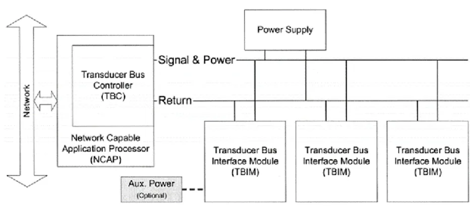
The purpose of this document [34] is to define an independent standard for interfacing multiple physically separated transducers, which allows time synchronization of data. This standard provides a minimum implementation that allows multidrop, hot swapping, self-identification and configuration of transducers that may not be located in the same enclosure, but are confident to a relatively small space. So, it allows transducers to be arrayed as nodes, on a multidrop transducer network, sharing a common pair of wires. It acts from the third to the fifth layer of the ISO/OSI model (Network, Transport and Session layers), as shown in Fig. 2.3, in a physical network wired as shown in Fig 2.4 (TBIM is the acronyms for Transducer Bus Interface Module).

Fig. 2.3 Model of the protocol stack.

2.2.5 IEEE 1451.4

This document [35] defines a mixed-mode transducer interface (MMI) for analog transducers with analog and digital operating modes. The standard provides two classes of communications for this Mixed-Mode:

 class 1: it sequentially transfers either a transducer signal or digital data;

 class 2: it uses separate connections to transfer transducer signals and digital data.

The TEDS model is also refined to allow above minimum of pertinent data to be stored in a physically small memory device, as required by tiny sensors.

2.2.6 IEEE 1451.5

The main purpose of this standard [36] is to define an open wireless transducer communication standard, which would accommodate various existing wireless technologies. Nowadays, wireless connections among electronic devices are increasingly used [37], so this document would enhance and support the acceptance of the wireless technology for transducers connectivity. It specifies radio specific protocols, thus, it requires a specific architecture, in which the NCAP and the WTIM (Wireless Transducer Interface Module) are equipped with one or more radio modules; the basic architecture is shown in Fig 2.5.

This standard specifies protocols for achieving this wireless interface: wireless standards such as 802.11 (WiFi) [38-41], 802.15.1 (Bluetooth) [42], 802.15.4 (ZigBee) [43], and 6LoWPAN [44-45]. It adopts necessary wireless interfaces and protocols to facilitate the use of technically differentiated, existing wireless technology solutions.

2.2.7 IEEE p1451.6

This is the project for edit the draft of the standard [46], which proposes a high-speed CAN open based Transducer Network Interface for Intrinsically Safe and non-Intrinsically Safe (IS) applications (Fig. 2.6). The proposed IEEE p1451.6 is a developing standard that defines a transducer-to-NCAP interface and TEDS. It adopts the CANopen device profile for measuring devices and closed-loop controllers. The application layer may be implemented free of licenses and royalties.

2.3 Issues

regarding

consistency

and

interoperability

There are some limitations in the standards and in the process of harmonizing the standards. “The main concern with regard to the

limitations is the consistency of standards, in terms of maintenance and management. It is a non-functional consideration, but crucial to determining whether a standard like IEEE 1451 can be more widely accepted and adopted by manufacturers” [49]. Other issues are related

to memory management, regarding, for example, storage of TEDS on tiny and low resources TIM.

In the last few years, these regulations of family of standards are being reviewed. Moreover, new standard versions will be also ISO (someone is already an active standard [50-51]), new projects are developing documents for other layers and, in the whole architecture, there is free space to allow new layers for other standardization proposals.

Chapter 3 The ISO/IEC/IEEE 21451.001 proposal, based on a segmentation and labeling algorithm

Chapter 3

The ISO/IEC/IEEE 21451.001 proposal,

based on a segmentation and labeling

algorithm

The IEEE 1451 family of standards is now evolving in the ISO/IEC/IEEE 21451 family of standards. In order to meet industry’s needs, this family of standards, responsible for the developing technology for smart transducers, is growing: some of the old IEEE 1451 standard versions are under revision, whereas new members are being developed. Currently working groups are convened to revise the 21451-1, 21451-2 and 21451-4, whereas other working groups are developing new layers not envisaged in the old version of the family of standards. These renewal and integration operations of new layers are made necessary by the will to enhance and facilitate device and data interoperability of distributed sensor networks.

As refers to a distributed sensor network, different considerations should be done to understand the complexity of this kind of system: main problems being generally reliability, communication bandwidth, and the big amount of data, with the related problem of flooding the central elaboration system with more information than it can process.

In a distributed sensing system, each sensor provides information about its surroundings to the central system. In different applications, the number of sensing elements in a network changes dynamically: the computational capabilities demand for the central elaboration system would increase with the number of sensors connected to the network. It would be better to manage a sensor network, with a variable number of connected nodes, without changing the computational requirements for the central system. So, in many applications, a part of the data processing is moved from the central elaboration unit, to the sensor

[53-55].

On the other hand, to optimize an algorithm for the particular application or hardware is totally in contrast with the main goal of the family of standard for smart transducers: to achieve device and data interoperability. Moreover, “the distributed measurement and control

(DMC) industry is migrating away from proprietary hardware and software platforms, in favor of open systems and standardized approaches” [56]. In order to propose a common preprocessing

technique that will reduce problems, related to channel bandwidth and reliability, without requiring big computational capabilities, the

Institute of Electrical and Electronic Engineers (IEEE) Instrumentation and Measurement Society’s (IMS) Technical Committee on Sensor Technology has developed a new document to

standardize this procedure. This document, identified with the code 21451.001 is now in the final step of developing before balloting and becoming a member of the ISO/IEC/IEEE 21451 family of standards. With this standard, smart transducers will ensure interoperability, using a common preprocessing technique and data structures.

3 ISO/IEC/IEEE 21451.001

3.1 A novel approach to signal preprocessing

ISO/IEC/IEEE 21451.001 is such a standard to regulate algorithms running on a transducer, a sensor or an actuator. The purpose is to facilitate the flow from sensor raw data processing to sensor information extraction and fusion, promoting and enhancing preprocessing on smart transducers.

The role of this preprocessing technique is to share part of the computational load needed in a sensor network among the nodes of the network, facing a smart transducer resource constrains, such as:

 low computational capabilities;  limited storage;

 short battery life;

 inadequate communication ability.

Moreover, needed algorithms must be flexible, depending on the sensors and the specific application.

So, the standard is structured in order to make different configurations possible:

1) the classic configuration where there is no data processing on sensors, and all the data are sent to the central system for processing. In this configuration there are low computational load constrains on sensors, whereas there is big traffic load of data in the network (Fig. 3.1 sensor 1).

2) A configuration where data are processed by sensors, and only results are used, sending them directly to a cloud or a fusion center. In this configuration there is a big computational load for sensors (which generally entails cost and complexity) but a lightened load for the network (Fig. 3.1 sensor 2).

3) Another configuration, where data are pre-processed by sensors and post-processed by central systems, which mitigate both the computational load required for sensors and the network traffic load (Fig. 3.1 sensor 3).

Using the hardware needed by the IEEE 21451 Transducer Interface Module, which requires a system based on a micro-controller, it is possible to implement, outside or directly on the TIM, data treatment services, providing extracted features rather than raw data for further analysis and processing.

The purpose of this preprocessing technique is to extract basic information from the raw signal, the same information that a human being could provide looking at the signal [57, 58]. This technique emulates a human observer, in the sense that it relates samples to infer a global behavior, detecting, for example, a minimum or a maximum, or inferring signal shape parameters.

The basis of this technique is the real-time segmentation and labeling (RTSAL) algorithm, which derives a data structure from the raw data [59].

3.2 A real time segmentation and labeling

algorithm

The basic idea of this algorithm is that it would describe the input signal as a human being could do: he would not enumerate all the acquired samples, but he would describe the shape of the signal, with only some noteworthy samples. This technique bases its analysis on the hypothesis that the needed information is not in any single sample, but it is contained in the relation among them. The aim of this technique is to store several meaningful samples, with which it is possible to keep several information about the signal, and from which is possible to extract several simple features. In this way, it is possible to have the same informative content, removing the redundancy of an oversampled input signal. Moreover, it implements a classification of the acquired raw samples, describing the signal trend.

The algorithm is described in the following paragraphs, divided into two parts: the segmentation and labeling phase.

3.2.1 Segmentation Step

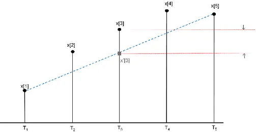
In this first step, the algorithm chooses the samples, to be saved from the raw samples, acquired with a constant sampling time. It works according to an input parameter, which is a kind of threshold for the algorithm: the interpolation error. Once it starts, it acquires the first three samples, and it linearly interpolates the first and the third sample, in order to calculate the amplitude the sample in the middle would have, if the signal were strictly linear. Then the algorithm calculates the difference between the amplitude of the interpolated sample and the amplitude of the sample acquired in that instant of time (Fig. 3.2).

At this point, the difference (d) is compared with the interpolation error, defined as a percentage value of the maximum value of the signal: if this difference does not exceed the interpolation error, the algorithm does not store the sample, and, once acquired two more samples, it interpolates the first and the fifth sample, computing the value of the third middle sample, to be compared with the real acquired sample. This algorithm goes on like this (Fig. 3.3, 3.4), increasing the interval in which it searches an important sample, until it finds a new one, or a maximum limit of comparisons is reached.

Fig. 3.2 The RTSAL algorithm makes linear interpolations and comparisons.

Whereas if d is bigger than the interpolation error, the algorithm stores the amplitude and the time position of the sample, considering this sample as important. These two values are stored in two different vectors (called “M”, for amplitude, and “T”, for time). When it stores a new sample, it begins again, starting from the last stored sample. Required operation for this algorithm are only sums, subtractions, and just one division by two for each iteration.

In Fig 3.5 there is the flowchart with an example version of the algorithm [59], where the interpolation error is compared with the parameter d computed as in (1), where i and k are two different counters, the first increased by one every time a new point is stored, whereas k is increased by two when a new point is not stored, to increase the interval.

d =

|

2

− 𝐒(𝑖 +

𝑘

2

)|

The interpolation error could be interpreted in different ways: it is a threshold for amplitude values, so it could be specified whether in the unit of the acquired signal, or coded to be compared directly with the output of the analog to digital converter (an entire number), or as a relative value. In the following paragraphs, the interpolation error value will be stated as a relative value of the full scale value of the sensor, except where expressly indicated (for the same reasoning, in simulations, signals have unitary maximum value).

3.2.2 Labeling Step

This step starts only when a new segment is saved. In this phase, the algorithm chooses a class in order to label the shape of the signal between two consecutive stored samples.

During the first phase, the algorithm saves also the sign of each computed difference d. When a new sample is stored, the tendency of the signal between this sample and the previous one is evaluated depending on the difference between these values, and on the majority of error sign accumulation. It uses ‘d’, ‘e’, ‘f’ and ‘g’ or ‘h’. If the algorithm saves a new value because the maximum length is reached, it uses linear classes ‘a’, ‘b’ and ‘c’, depending on the slope. A graph of labeling process is shown in Fig. 3.6.

For each sample, the class is stored in a third vector, called “C”: in this vector all information about the signal shape is saved. Several signal parameters could be easily extracted by processing the elements of this vector [59]; it has not any relation with amplitude or time scales, it stores only a qualitative information. The most common classes are

The RTSAL algorithm requires only few operations: one sum, one subtraction, and one division by two (which could be easily implemented as a shift in a binary register) each iteration. So, it is easy to implement on micro-controllers and can run in real time.

3.3 Draft proposal for a recommended practice

The set of vectors mark, class and time, in short MCT, is the basic structure on which are grounded algorithms proposed by the draft of this recommended practice. The dimension of a single variable is fixed, whereas the size of the vectors depends on the RAM dedicated for this practice.

The amplitude value, stored in the mark vector, could be an unsigned integer, if it contains the output value of the analog to digital converter (2 bytes, UInt16). The class value, stored in the class vector, as already explained in the previous paragraph, can be only one of eight different values (1 byte, UInt8). The time stamp, stored in the time vector, works as a time reference (millisecond from midnight, 4 bytes variable, UInt32). These vectors could be continuously generated and stored in circular buffer structures.

Algorithms included in this recommended practice are divided in two layers: the first layer algorithms take the MCT structure as an input, whereas the second layer algorithms also take results of the first layer algorithms as an input. The algorithms in the first layer are for the extraction of simple and basic properties or parameters: these

algorithms are the exponential detection, the noise detection, the

impulsive noise detection, the sinusoidal pattern detection, the tendency estimation and the mean estimation. The algorithms in the second layer

are conceived for the computation of complex parameters: these algorithms are the steady state value estimation, smart filtering and

compression. There is also a user defined application code block, which

allows manufactures or users to include their own algorithms based on

MCT vectors and/or first layer algorithms. This structure (Fig. 3.7) is

flexible, meaning that it could be implemented on different levels, choosing layers to be implemented, depending on the hardware and other constraints.

3.4 First layer algorithms

3.4.1

Exponential Pattern Detection

The aim of this function is to detect an exponential shape, with a fixed number of consecutive segments, using MCT vectors. The exponential detection function searches through the class vector, looking for consecutive equal classes. The number of times that a class has to be consecutively found is the only input parameter for this

Fig. 3.9 Example of exponential patter detection, class ‘g’ (interpolation error 0.03). On the left the acquired signal, on the right, in red dots, the segments stored in the MCT structure.

Fig. 3.10 Example of exponential patter detection, class ‘d’ (interpolation error 0.03). On the left the acquired signal, on the right, in red dots, the segments stored in the MCT structure.

noise. Moreover, it could be possible to implement a periodic noise detection: standard deviation of the noise is an indicator of random noise. Computing the mean and the standard deviation of periods observed in the temporal window, the algorithm calculates the ratio, and

compares this value with the input parameter

ThresholdPeriodicDetection. If this ratio is lower than the fixed

threshold level, the algorithm calculates the period of the signal, and it returns this value as an output. Below some examples of different Matlab® simulation are shown (Fig. 3.11 and 3.12).

Fig. 3.11 Example of sinusoidal waveform, not flagged as “Noisy” (interpolation error = 0.1, signal frequency = 30 Hz, NoisyPeriod = 1ms, AmountNoisy = 5, SNR = 40 dB).

3.4.3 Impulsive Noise Detection

This function considers as an impulsive noise a significant change of the amplitude in two consecutive segments: when it finds a minimum or a maximum, it computes the amplitude change, taking into account the amplitude of the segment before the minimum or the maximum. Input parameter for this function is the ImpulseThreshold, which defines a threshold for the amplitude differences. The Impulsive Noise Detection function browses the entire class vector, looking for maxima and minima and, when it finds one, it computes the amplitude difference between this value and the previous one, and then compares this last value with the threshold. This algorithm could return several different information about the impulse, like position in the time vector, amplitude, duration or area. As an example, different simulation results are reported (Fig. 3.13 and 3.14)

Fig. 3.12 Example of sinusoidal waveform, flagged as “Noisy” (interpolation error = 0.1, signal frequency = 30 Hz, NoisyPeriod = 1ms, AmountNoisy = 5, SNR = 20 dB).

Fig. 3.13 Example of sinusoidal waveform with an impulse added (interpolation error = 0.1, signal frequency = 15 Hz, ImpulsiveThreshold = 0.3).

Fig. 3.14 Example of exponential waveform with periodic impulses added. (interpolation error = 0.1, signal frequency = 15 Hz, ImpulsiveThreshold = 0.3).

3.4.4 Sinusoidal Pattern Detection

The sinusoidal pattern detection algorithm is based on the pattern of classes shown by a sinusoidal waveform, saved in the MCT structure with the segmentation and labeling algorithm. The sinusoidal pattern of classes is composed of segments ‘g-e-f-d’: the classes has to be in this order to assume that the input signal is a sinusoidal waveform. The algorithm search through the class vector and, if the pattern of classes is correct, it returns the period of the sine, computed using the value of the time vector of two consecutive maximum segments, and it checks if the input signal has damped or undamped oscillations. An example of Matlab® simulation is shown (Fig. 3.15).

In order to clarify the role of the interpolation error on the conversion in MCT by the segmentation and labeling algorithm, results of the sinusoidal pattern detection function are shown in the top of the Fig. 3.16. In this chart, red dots are for a correct pattern labeled by the algorithm, whereas blue dots are for an incorrect pattern for a sinusoidal waveform: this analysis is carried fixing the input signal, varying the interpolation error used to segment the input signal, and the signal to noise ratio with which the signal is generated. As an example, in the center and in the bottom of Fig. 3.16, two different cases of

Fig. 3.15 Segments saved by the segmentation and labeling algorithm of an ideal sinusoidal waveform, with interpolation error equal to 0.06 (signal frequency = 60).

Fig. 3.16 Red dots, in the upper picture, point out cases in which the right sequence of classes is stored, as a function of signal to noise ratio and interpolation error.

3.4.5 Tendency Estimation

Tendency of input signal is computed processing only maximum and minimum segments: the algorithm applies formula (2) on a vector made by maximum segments, and formula (3) on a vector made by minimum segments. The number of segments taken into account depends on application: it is possible to run this algorithm when the

MCT buffer is full, or it is possible to run this algorithm on the

segments acquired in a fixed time window. These formulas return a normalized factor which gives information about trends, and their span is from -1 to +1. If the tendency of maxima is positive and the tendency of minima is negative, the signal grows its peak to peak amplitude (example: unstable oscillations), whereas, if the tendency of maxima is negative and the tendency of minima is positive, the signal diminishes (example: damped oscillations). In addiction, the average of these two factors returns information about the global tendency of the signal.

Trendmax = ∑_𝑚𝑎𝑥(𝑇_𝑥+1−𝑇_𝑥)(𝑀_𝑥+1−𝑀_𝑥) ∑_𝑚𝑎𝑥(𝑇_𝑥+1−𝑇_𝑥)|𝑀_𝑥+1−𝑀_𝑥| (2) Trendmin = ∑𝑚𝑖𝑛(𝑇𝑥+1−𝑇𝑥)(𝑀𝑥+1−𝑀𝑥) ∑_𝑚𝑖𝑛(𝑇_𝑥+1−𝑇_𝑥)|𝑀_𝑥+1−𝑀_𝑥| (3)

3.4.6 Mean Estimation

One of the most important algorithms, in different applications, is the mean computation. This function could be implemented in different ways: the mean of the vector M of the MCT structure, take into account even values of the vector T, because samples stored in the MCT structure are not equally spaced in time (see par. 4.2.5). Even in this case, the number of segments taken into account depends on the application (running this algorithm when the MCT buffer is full, or when segments acquired in a fixed time window are stored).

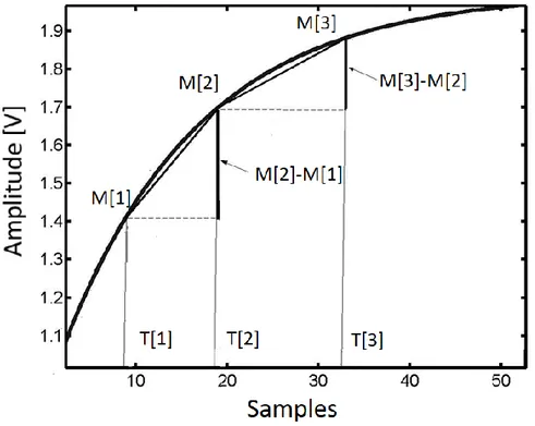
x(t) = 𝑋𝑀 - [𝑋𝑀− 𝑋0]𝑒−𝑡 𝑇⁄ (4)

The idea is to approximate the shape of the exponential between two consecutive segments in the MCT structure with a linear shape: the samples stored in the MCT structure are on the exponential curve, whereas the value of XM, the steady state value, and T, the time constant,

are unknown. The derivate of x(t) at t=0 is:

𝑑𝑥

𝑑𝑡

|

𝑋_𝑀− 𝑋₀

𝑇 (5)

The derivate can be approximated with the slope of segments at the starting points. Considering:

𝑋𝑀−𝑀[1] 𝑇

=

= 𝑀

=

= 𝑀

where Ma and Mb are slopes in the starting point. Solving (6) and (7) for XM:

𝑋

=

𝑀𝑎−𝑀𝑏 (8)

The steady state value XM can be estimated, without knowing time constant T.

3.5.2 Smart Filtering

Basing on the MCT data structure, it is possible to reconstruct an approximation of the sampled signal. The starting acquired signal is included in an interval smaller than the interpolation error value used in the segmentation step. The reconstructed signal is a combination of a scaled and shifted version of two generating functions:

signal has to assume values of these essential samples. Spline polynomials can be used to reconstruct the signal within the segment. The two generating functions converge to a straight line between essential samples, in case of linear interpolation reconstruction.

A low pass filtering effect can be achieved, applying repeatedly the

RTSAL algorithm on an acquired signal: once obtained the MCT

structure, from the input samples, it is possible to reconstruct the signal using a linear interpolation, and then, applying the RTSAL on this reconstructed signal, it is possible to obtain a new MCT structure. This new set of vectors, M’C’T’, has lost part of the high frequency content, and this principle can be iterated, in order to remove some unwanted high frequency components or noise.

Applying RTSAL algorithm, the number of local minima and maxima on a fixed time window can be used as a control variable for the number of iteration. In the following picture (Fig. 3.19), a flow chart of the proposed method is shown. The variable N is the total number of minima and maxima of the time window analyzed by the RTSAL algorithm in the current iteration, whereas N’ is the total number of minima and maxima in the previous one. This procedure generates an

MCT data structure for the input signal, after that it reconstructs the

signal with a linear interpolation, with the same time step with which the input signal is acquired, and then it computes the value of R (R = (N – N’)/N’). If R is smaller than 0.1, the procedure is repeated. An example of application is reported in Fig. 3.20, with a Matlab® simulation.

3.5.3 Compression

The RTSAL algorithm achieves a conversion of the input vector of samples in a data structure, but it does not mean that there are benefits in all the cases. A correct choice of the interpolation error could allow both enough information and data size reduction, but it requires to know the typical input signals. In order to obtain a compression, even when the domain of the input signal is unknown, an automatic procedure to make a reasonable choice of the interpolation error is needed. A large

Fig. 3.20 Filtering: input signal (top), reconstructed signal after 3 iterations (middle), and reconstructed signal after 8 iteration (bottom).

value of the interpolation error leads to high compression rate and compression error, whereas smaller value of the interpolation error results in lower compression rate and error. Input parameter for this procedure are l, the changing step for the interpolation error value, and the Rmin, lower bound for the correlation coefficient. This procedure

starts applying the RTSAL algorithm with a relative high interpolation

error value, it process the MCT output in order to reconstruct the signal

(for example with a linear interpolation), and then it computes the correlation between the input signal and the reconstructed one. If this correlation is smaller than the value of Rmin, it reiterates this procedure,

once decreased the interpolation error of a value equal to l. When the correlation is appropriate, it returns the new data structure M’C’T’. A flow chart of this procedure is reported (Fig. 3.21).