1
Student number n. 0000901857
ALMA MATER STUDIORUM
UNIVERSITY OF BOLOGNA
DEPARTMENT OF INGEGNERIA DELL’INFORMAZIONE
MASTER DEGREE IN ELECTRONIC ENGINEERING
Deep Neural Recovery for Compressed Imaging
Dissertation on Signal Processing
Supervisor Presented by
Prof. Riccardo Rovatti Filippo Martinini
Co-supervisor Prof. Mauro Mangia Dottor Alex Marchioni
Session 10/3/2021 Academic year 2020/2021
2
TABLE OF CONTENT
1 MOTIVATIONS... 6 2 INTRODUCTION ... 8 2.1 INTRODUCTION ... 8 2.2 MRI... 10 2.3 COMPRESSED SENSING ... 12 2.4 IMAGE PROCESSING ... 162.5 ARTIFICIAL INTELLIGENCE,MACHINE LEARNING ... 17
2.6 NEURAL NETWORKS ... 19
3 LOUPE ... 27
3.1 DECODER:U-NET ... 28
3.2 ENCODER:ADAPTIVE UNDER-SAMPLING ... 31
3.3 AUTOENCODER ... 37
3.4 RESULTS AND CONCLUSIONS... 38
3.5 PROBLEMS AND HOW TO IMPROVE LOUPE. ... 41
4 CONTRIBUTIONS ... 43
4.1 PRANCING PONY: GRADUAL APPROXIMATION OF 𝒔 ... 43
4.2 FLASHBACK: TRAINING ON THE MINIMIZATION OF THE ERROR OF THE RECONSTRUCTED K-SPACE IMAGE. ... 46
4.3 FLASHBACK AS SELF-ASSESSMENT. ... 48
4.4 TIFT: TRAINABLE INVERSE FOURIER TRANSFORM. ... 49
4.5 BACK TO THE FUTURE... 52
5 RESULTS ... 55
5.1 PRESENTATION OF THE DATASET ... 55
5.2 RESULTS OF ORIGINAL LOUPE AND NORM TUNING. ... 57
5.3 TUNING OF SLOPE 𝒔 IN 𝝈𝒔 AND PRANCING PONY. ... 59
5.4 FLASHBACK USED AS TRAINING REGULARIZATION TERM. ... 62
5.5 TIFT. ... 65
5.6 BACK TO THE FUTURE... 67
5.7 BACK TO THE FUTURE BUILT WITH TFT AND TIFT. ... 68
5.8 FLASHBACK USED AS SELF-ASSESSMENT. ... 69
5.9 RESULTS OF LOUPE WITH ALL CONTRIBUTIONS. ... 77
5.10 FUTURE RESEARCH ... 81
4
TABLE OF FIGURES
Figure 2-1 - example of MRI scan ... 10
Figure 2-2 - Example of under-sampling ... 13
Figure 2-3 - Edge detection on MRI ... 17
Figure 2-4 - scheme of a neural network made with Dense layers ... 20
Figure 2-5 - Example of convolutional layer ... 22
Figure 2-6 - Example of pooling layer ... 22
Figure 2-7 - Architecture of AlexNet ... 23
Figure 2-8 - Architecture of VGG ... 24
Figure 2-9 - Architecture of GoogleNet ... 24
Figure 2-10 - Architecture of ResNet ... 24
Figure 3-1 - Autoencoder representation ... 27
Figure 3-2 - DECODER structure ... 29
Figure 3-3 - U-NET scheme ... 30
Figure 3-4 - U-NET used in LOUPE ... 31
Figure 3-5 - DECODER scheme ... 32
Figure 3-6 - Sigmoid function ... 34
Figure 3-7 - Layers of loupe ... 37
Figure 3-8 - Layers of loupe with formulas ... 38
Figure 3-9 Results of LOUPE trained on knee dataset ... 40
Figure 3-10 LOUPE example of reconstruction ... 41
Figure 4-1 - Scheme of LOUPE with Flashback ... 48
Figure 4-2 - Super dense scheme ... 51
Figure 4-3 - TIFT scheme ... 51
Figure 4-4 scheme of back to the future ... 53
Figure 4-5 scheme of back to the future generalized ... 53
5
Figure 5-1 Example of MRI scans from the data set ... 56
Figure 5-2 LOUPE L1 vs LOUPE L2 ... 57
Figure 5-3 MRI scans encoded and decoded by LOUPE ... 59
Figure 5-4 s tuning: train ... 61
Figure 5-5 Distribution of the mask pixels ... 62
Figure 5-6 Flashback PSNR over phi for a set of ALPHAS ... 63
Figure 5-7 Flashback: phi tuning ... 64
Figure 5-8 Flashback: tuning of the norm ... 65
Figure 5-9 without TIFT vs TIFT ... 66
Figure 5-10 LOUPE vs LOUPE and back to the future ... 68
Figure 5-11 LOUPE with back to the future built using TFT and TIFT ... 69
Figure 5-12 Squiddy plot: reconstruction error vs Flashback ... 71
Figure 5-13 Squiddy plot: fitting with polynomial of degree greater than 1 ... 72
Figure 5-14 histogram of the predicted MSE error ... 73
Figure 5-15 histogram of the predicted MAE error ... 73
Figure 5-16 histogram of the predicted PSNR error ... 74
Figure 5-17 Distribution of the error on reconstructed pixels ... 76
Figure 5-18 LOUPE with all contributions vs original LOUPE ... 77
Figure 5-19 LOUPE trained with all contributions but Prancing Pony ... 78
Figure 5-20 LOUPE trained with Flashback and Back to the Future ... 79
6
1 Motivations
Since the discovery of the firestone mankind developed fast enough, we invented the wheel, we found a good approximation of 𝜋, we created really fast cars, we landed on the moon… We developed fast enough so that we do not feel we actually have so many years of evolution behind us, till nowadays where we have internet, artificial-intelligence-based systems and a too much pollution in the air we cannot continue ignoring it.
At the dawn of civilization man dreamt of mighty gods who could control all the elements and who could interact with death, life and so on. Man created stories and religions based on what they could only imagine, until the day someone did what before was just ‘reasonably impossible'.
That is what always happened: you cannot do something you would really love to, so you make up a tail. The day the tail turns out to be reality, you move on, on something you still cannot do.
Man always chased future by inventing stories. Nowadays we can still hear and read about the long-forgotten stories of the past and laugh about them, but when what is now technology was only magic people were fascinated by it, people imagined the problem, spent hours arguing about the complications and studied it. Stories always gave an input, a kick-off into the minds of great scientists, they gave a target, maybe an impossible one, but they gave a target to the people.
The great sci-fi writer Arthur C. Clarke summarized the topic into 3 laws[1]:
Clarke's First Law: When a distinguished but elderly scientist states that something
is possible, he is almost certainly right. When he states that something is impossible, he is very probably wrong. (Clarke)
Clarke's Second Law: The only way of discovering the limits of the possible is to
venture a little way past them into the impossible. (Clarke)
Clarke's Third Law: Any sufficiently advanced technology is indistinguishable
from magic. (Clarke)
What is going to be discussed in this work is not something concerning the future of humankind, is not something unimaginable, something only Arthur C. Clarke could write, but another little step toward the progress, a thing that had not be created jet and was only waiting for someone to be invented.
7
What brought Earthmen to we call ‘our society’, is the same that brought me here: an inspiration.
I am convinced that we owe so much, maybe we owe more than what I think, to the imagination of the people who wrote the story, who directed the film, who played the poem, who… that has been inspiring us, from the first to the last human being.
What we, engineers, are, is the link between the present and the future: a future that has already been written by our favourite sci-fi writer. We, engineers, work to hear someone call, one day, ‘reality’, what for us, now, is science fiction.
Without us, engineers, future would be tediously possible, and magic would just remain magic and, at last, Clarke would have never discovered his third law.
Finally, my motivation is a science fiction future where positronic robots live alongside humans and Earth is not the only inhabited world in the universe and people can live up to 400 years. What this project discusses is not directly linked with robots and extended life, but I like to think that it is another step, even if it is a short one, toward Asimov ‘novels.
8
2 Introduction
This introduction chapter will be split in the following way: 1. Introduction 2. MRI 3. Compressed Sensing 4. Image Processing 5. Artificial Intelligence 6. Neural Network
This sequence of targets will introduce step by step the state-of-art method that this work is going to improve.
In chapter two the state of the art will be discussed and explained in depth. In chapter three the new contributions will be discussed.
In chapter four the results of the contributions will be shown.
2.1 Introduction
The story of electrical engineering begins when, around 3700 years ago, someone used to play with eels, to pet a cat’s fur and to rub amber. These ancient engineers, having no materials but their dreams used their own body as a conductor. As the work of an engineer has always been a hard one, especially in those times, nobody wanted to apply for it and electricity remained quite a curiosity for many millennia and nobody cared of studying it.
In 1700 glimpses of a resting curiosity emerged, and some bizarre inventions came out of the cylinder appearing as magic to whom didn’t know of the third law of Clarke [1]. The century continued flawlessly until a real invention ‘shocked’ the world: Volta invented the battery, it was 1800 and the world could not discard electricity anymore, it became clear that electricity was useful, and it was in the same way clear, that it was possible to make money out of it and the researchers appeared.
In the nineteenth century the interest on developing new tools using electricity grew rapidly and at the beginning of 1900 incredible discoveries, as the Marconi’s radio, were already commercials.
The story of transistors dates to 1947/1948 when Bardeen, Brattain and Shockley invented the first types of transistors. They could probably not imagine, but they moved humanity into the future, probably further than almost everybody body else before them. That day they announced
9
their discovery the ‘transistor era’ became real. Transistors found, in a short time, an incredible interest. A large group of researchers grew in few years, improvements and applications were close to see the light.
Everything started few lines ago, it seems impossible, but now it is 20 June 1969: and humanity lands on the moon. Every time it had to seem a short step, in particular for the guy who liked to fish and pet his eels. But in the end, a small step became part of a huge jump: such a huge jump that we reached the moon!
Since the world showed increased interest in science, it has never been only technological inventions ending in themself, but it has been a chain of improvements in every aspect. The developing of new technologies created new possibilities for the market, economy systems grew and wealthier states guaranteed safer lives[2]. Medicine, following this trend, engulfed the scientific method and obtained great improvements. With an increasing life expectancy, and a supporting strong economy, always more people gained the possibility to study and to apply new ideas to the world. Market, social life, politics, literature, medicine… everything, received contributions and gave contributions.
Science created a closed loop feedback: a society inside which we still consume, live, study and fuel it.
Of course, there is an important implicit consequence: the degree of improvements must always grow. We live in an old society, a society that has always grown. We reached a high level of complexity in almost every field of research. At the point where we are, innovative ideas and complex schemes must always be tried to solve new problems.
When doctors, at the beginning of 1970, reached a high level of understanding of the human body they faced the problem of: ‘What to do, now, to improve?’. Doctors by themselves could not find out what was the next step, but together with engineers they achieved the construction of the first MRI. It was a huge problem of great complexity and they had to tackle it, they had to improve the state of the art and at the end they succeeded.
It happened, around 2010, that while MRIs were working fine and doctors started using the new devices, that the MRIs themself showed their limitations. Once more the world asked for more developments, and once again engineers replied, with a new revolutionary idea: compressed sensing. Compressed sensing achieved the goal and perfectly adapted.
It is 2021 now and we have been called for another improvement, can we still do better? The answer is Yes, well, the answer is always Yes, it has to be Yes.
10
This work draws its new key element from a recently developed field of study: Deep Learning, applying it to the well-known compressed sensing method.
This work aims to improve a novel algorithm for accelerating MRI acquisition via compressed sensing using new deep learning model that specializes on the details of the class of the acquired data.
2.2 MRI
Magnetic resonance imaging (MRI) is a medical imaging technique and diagnostic tool in radiology based on the Nuclear Magnetic Resonance (NMR).
MRI is widely used worldwide as one of the main instruments to have accurate images of sections of the body. Relying on MRI doctors can guarantee to the patients, in depth analysis of their health problems.
FIGURE 2-1- EXAMPLE OF MRI SCAN
MRI is a main subject of research in the world, in 2020 7782 paper have been published on ‘Scopus’ containing the keyword ‘MRI’, of which 997 are classified as engineering research [3][available at 01/01/2021].
MRI market is constantly increasing in many countries, being MRI a main technology for medical purposes for both public and private health. For example, between 1990 and 2007 number of MRI per one million inhabitants varied from 1.8 to 15.3 in Finland[4].
11
NMR is the phenomenon that denotes the induced current on a magnetic coil obtained by emission of a magnetic current of an object on which another magnetic field was previously applied.
1. A sample has been placed in an ideal uniform magnetic field produced by a magnetic coil.
2. A current is applied for a short time to the coil, an oscillation of the magnetic field occurs in the sample.
3. Some particles have interesting properties related on absorption of energy given by a magnetic field. If the sample is, for example, hydrogen nuclei, the hydrogen absorbs some energy.
4. If the sample has absorbed energy, some of this energy will be emitted as an electromagnetic wave which frequencies lies in the radiofrequency (RF), in the interval of [3𝐾, 300𝐺]𝐻𝑧.
5. The coil will be affected by the same magnetic field produced by the sample and a current will appear on the coil, oscillating at the same frequency of the RF signal. The current that is measured is called NMR signal.
More in-depth explanation:
Relaxation is the process by which any excited particles relax back to its equilibrium state, after a magnetic field gave energy to it. It can be divided into two separate processes: Longitudinal relaxation (T1) and Transverse relaxation (T2).
Every tissue has its relaxation times. In MRI is possible to measure both T1 and T2 to understand what element is hidden inside the body that is analysed. For example, it known that: T1 is always longer than T2. Liquids have very long T1 and T2 values while dense solids have very short T2 values.
A spin echo is produced by two successive RF-pulses (usually 90° and 180°) that create a detectable signal called the echo.
Tissues have different T1 and T2. Signal intensity depends on these parameters: one aims to maximize the contrast between tissues focusing on one of these parameters.
To detect the location of NMR, MRI has three gradient coils, one for each orthogonal axis. A gradient coil produces a small magnetic gradient (compared to the main magnetic field). By producing a gradient is possible to produce the exact magnetic field to be absorbed by the
12
particle only in a small section of the body (such as 1-2 mm thick). By adjusting the intensities along the three axis is possible to point to a region of the body and scan only such a region. MRI uses a frequency encoding to return the output: MRI generates a precise frequency magnetic signal and reads the relaxation time of the slice of the body which resonates. This means that the output of MRI is not a normal image but is the Fourier transformation of the image. To obtain the final image is necessary to apply FFT algorithm to the MRI output. MRI has been studied since its first invention with high interest by the scientific community and many improvements have been done. Here is a list of the pros and of the cons that still nowadays require investigations:
Pros:
1. non-invasive and 3D modelling of the body. 2. no ionization radiations.
3. nice spatial resolution.
4. can scan a wide range of internal tissues. Cons:
1. is an expensive machine.
2. long-time are required to scan, that leads to artifacts in the image.
3. if patient has metals inside his body, MRI cannot be done due to interaction of metal with magnetic field [5].
4. when on is very loud and is not designed to be comfortable for the patient. Most of the above introduction to MRI has been inspired by [6].
The biggest usage problem is the long scan time. One of the first researcher who studied the problem finding a good algorithm for speeding up the acquisition is Griswold et al. with his paper [7] where he proposed a fast configuration for autocalibration acquisitions.
2.3 Compressed Sensing
Compressed Sensing (CS) [8] is a recent area of study, it aims to shorten the time duration of the acquisition, the power consumption or it aims to overwhelm the hardware limitations of a sensor by reducing the sampled data and by reconstructing the incomplete data in another moment.
13
A classically correct acquisition of a data requires the sampling of a source of the signal with a sampling frequency 𝑓𝑠 at least higher than two times the maximum frequency 𝑓𝑚𝑎𝑥 of the signal itself. This rule is known as the Nyquist theorem and is one the first fundamental theorems every electronical engineer studies. Respecting the Nyquist theorem is usually so important that before acquiring the signal, the signal itself is filtered to cut out every frequency that would escape the limit of the 𝑓𝑠
2.
The demonstration that 𝑓𝑠 > 2𝑓𝑚𝑎𝑥 to correctly reconstruct the signal is intuitive:
Considering a sine wave of frequency 𝑓𝑠𝑖𝑛𝑒 = 𝑓𝑚𝑎𝑥 and sampling it by a frequency that do not respect the Nyquist theorem will lead to obtain a set of samples that if reconstructed return a different signal than the sine wave: the reconstructed signal will have more and different frequency components than the expected ones.
FIGURE 2-2-EXAMPLE OF UNDER-SAMPLING
When a signal is sampled using a frequency 𝑓𝑠 lower than 2𝑓𝑚𝑎𝑥, we address the phenomenon as ‘under-sampling’. If under-sampling is carried on a complex signal (not just on a sine wave) frequencies will interfere in reconstruction leading to errors known as ‘aliasing’ errors. The phenomenon itself is called ‘aliasing’. Even if ‘small number of linear measurements’ are available, is possible to reconstruct the data trying to minimize the error[9].
The key idea of CS[10] is to under-sample, helping saving energy and time, obtaining data that cannot be normally reconstructed, but that require more advanced algorithms to be reconstructed.
Mathematically the under-sample operation is a simple linear operation[11], given a vector 𝑥 ∈ ℝ𝑛 and 𝑦 ∈ ℝ𝑚 called ‘sample’ and ‘compressed sample’, with 𝑛 < 𝑚 , the under-sample matrix is a matrix 𝐴 ∈ ℝ𝑛×𝑚:
14 𝑦 = 𝐴𝑥
This is also called ENCODING. Computational cost and complexity are low, allowing to obtain an easy task. The problem lies in the reconstruction of 𝑥 given 𝑦, that is called DECODING. The reconstruction is critical because 𝐴 is a rectangular method and 𝐴−1 allows infinite different solutions.
A naïve way to obtain 𝑥 could be to compute the pseudo-inverse of 𝐴, but this method could not guarantee to retrieve the original sample. Instead of working on the minimization of ‖𝑥‖𝐿2 𝑠𝑢𝑐ℎ 𝑡ℎ𝑎𝑡 ‖𝑦 − 𝐴𝑥‖𝐿2 < 𝜂, CS works on the hypothesis of sparsity of the signal 𝑥 and
exploits it.
Assuming 𝑥 ∈ ℝ𝑛 is k-sparse, it can be represented with a sparse representation 𝑥 = 𝐷𝜉 where 𝜉 has at max 𝑘 non-zero elements and the encoding can be written as:
𝑦 = 𝐵𝜉 Where 𝐵 = 𝐴𝐷.
𝜉 is DENSE, meaning that even if it is smaller compared to 𝑥 it contains the same information of 𝑥. The problem requires the knowledge of the sparsity 𝑘 and of the space 𝐷 (also called ‘dictionary’) where the signal is sparse, that means that is necessary to study the signal and extract some features out of it. An example could be 𝑥 = sin(2𝜋𝑓𝑡) that has a sparse representation in the frequency domain: 𝑥 = 𝐹𝜉 where 𝐹 is a Fourier operator and 𝜉 is vector with a unique non-zero element that is the frequency 𝑓 of sin(2𝜋𝑓𝑡).
Given these hypothesis CS searches the sparsest vector 𝜉̂:
𝜉̂ = argmin(‖𝜉‖𝐿0) 𝑠𝑢𝑐ℎ 𝑡ℎ𝑎𝑡: ‖𝑦 − 𝐵𝜉‖𝐿2 < 𝜂
This problem is NP-hard [12] add citation on NP-hard, so it is requiring to solve, so the request is lightened by requiring:
𝜉̂ = argmin(‖𝜉‖𝐿1) 𝑠𝑢𝑐ℎ 𝑡ℎ𝑎𝑡: ‖𝑦 − 𝐵𝜉‖𝐿2 < 𝜂
This is possible only under certain conditions, called ‘Restricted Isometry Constraint’ (RIP)[13] [14] that requires the matrix 𝐵 to be a ‘quasi-isometry’. The great power of CS is that it guarantees that matrix 𝐵 respects the RIP condition whenever:
𝐴 ℎ𝑎𝑠 𝐴𝑖,𝑗 ∼ 𝑁(0,1) 𝑤𝑖𝑡ℎ 𝑖 = 0, … , 𝑛 − 1; 𝑗 = 0, … , 𝑚 − 1 𝑎𝑛𝑑 𝑚 = 𝑂 (𝑘 log (𝑛 𝑘))
15
Without any constraint on 𝐷. Once obtained 𝜉̂ the original signal is reconstructed by computing 𝑥̂ = 𝐷𝜉̂.
The given introduction to CS gives the guarantee that CS works fine for a sparse vector and it is robust for generic signals. CS can be further improved for real application by specializing the method and adapting it in two main ways:
1. Adapting CS to a particular class of signal by improving the under-sampling (encoding). 2. Adapting CS to obtain a better reconstruction, given the under-sampled signal
(decoding).
It has been demonstrated that 𝐴 can be also a sub-gaussian matrix and respects RIP condition, meaning that the ENCODING procedure can be even easier than it already has been shown. An interesting case is when 𝐴 is a random under-sampling of 𝐼 (identity matrix): 𝐵 is simplified but the generality of the classes of sparse signals on which CS now works is reduced. CS can be adapted to specific classes of signals by the use of different and more convenient 𝐵 that are not, in general, valid.
CS can simplify the acquisition, but at the same time can adds complexity to the reconstruction, making it an ideal method to apply in contests where resources at acquisition time are low while the receiver has computational power.
CS is a huge helper for MRI acquisitions: CS relaxes the acquisitions of MRI to speed up the scans and helps preventing errors caused by accidental movements of the patient and reducing the cost of procedures.
CS algorithm applied to MRI have shown acceleration up to 80% [15] and made feasible new medical treatments such as the first pass cardiac perfusion MRI [16]. The same work demonstrated feasibility of 8-time acceleration in vivo imaging.
MRI related to CS is a main subject of research in the world, in 2020 34 engineering papers have been published on ‘Scopus’ containing both the keyword ‘MRI’ and ‘compressed sensing’[3].
To under-sample in an MRI machine means to stimulate the region of the body with less frequencies and obtain a less dense space representation of the body. An under-sampled k-space image do not respect the Nyquist theorem: CS must prevent the aliasing phenomenon from reducing the quality of the reconstructed image.
16
Jong Chul Ye in his paper ‘Compressed sensing in MRI: a review from signal processing perspective’ [17] delineates the evolution of many algorithms through the last decade. Some of the most important works, who reached interesting results:
LORAKS [18] demonstrates that k-space data can also be mapped to low-rank matrices when the image has limited spatial support or slowly varying phase and obtain interesting results. ALOHA [19] is a generalized approach of LORAKS that continues the research and widen the usability of the method.
These two methods reached considerable results and are usually used as benchmarks.
2.4 Image Processing
Image processing is the study of the images from a signal processing point of view. Image processing is a method to perform some operations on an image, in order to get an enhanced image or to extract some useful information from it. Image processing is an incredibly important discipline that is growing fast but it is already a wide area of study. For the sake of clarity in this work only 2D images having 8-bit quality will be treated.
In image processing 2D grayscale images are treated as tensors with 𝑠ℎ𝑎𝑝𝑒 = (1, 𝑛, 𝑚, 1) where the first dimension 𝑠ℎ𝑎𝑝𝑒[0] means that the image is 2D, the second and the third dimensions, 𝑠ℎ𝑎𝑝𝑒[1,2], stand for the 𝑤𝑖𝑑𝑡ℎ, ℎ𝑒𝑖𝑔ℎ of the image (number of pixels) and the last dimension 𝑠ℎ𝑎𝑝𝑒[3] stands for the number of channel of the image: if 𝑠ℎ𝑎𝑝𝑒[3] = 1 the image is a grayscale image, if 𝑠ℎ𝑎𝑝𝑒[3] = 3 the image is an RGB image.
Usually every pixel (value of the tensor) of the image is a value that lives inside the natural set ℕ in the range [0, 255], but the values are usually normalized between [0,1].
Image processing has many and variable targets, two of its major aims are: 1. Image manipulation.
2. Features extraction.
A classical algorithm of image manipulation is the blurring effect, used to reduce details and noise.
The gaussian blur consists in a ‘sliding window’ of dimension (𝑙, 𝑘), which elements are the result of the gaussian function 𝐺(𝑥, 𝑦) = 1
2∗𝜋∗𝜎2𝑒
−(𝑥2−𝑦2)
2∗𝜎2 , that slides all over the image and that
returns for every pixel of the image the result of the 2D discrete convolution of the window with the current window of pixels the sliding window is sliding on.
17
A classical task of feature extraction algorithms is the ‘edge detection’ task.
Edge detection searches the part in the image that a human could consider the edges of shapes. An image with its values in the continuous range [0,1] is taken as input and the output is another image with the same dimensions of the input image but whom pixels could only assume two values: (0,1), where 0 represents the edge and 1 represents the background.
Edge detection[20] is only a branch, one of the first and most important, of the field of image processing, but is a significative example that shows how the subject is constantly growing and updated.
Image processing is used in many applications, also in MRI, to filter and improve the reconstructed image.
It is possible that both a gaussian filter and edge detection will be applied to the MRI image to get rid of some noise and then to extract the position of some interesting portion of the image (e.g., the edges of a broken bone).
FIGURE 2-3-EDGE DETECTION ON MRI
CS also makes wide use of image processing algorithms to improve its performances when it aims to reconstruct under-sampled image signals[21].
2.5 Artificial Intelligence, Machine Learning
18
Defining what an intelligent machine is, is not an easy task, there exist papers whom purpose is to investigate the complexity of the meaning of AI. A recent published paper that analyses the problem is ‘On Defining Artificial Intelligence’. The paper proposes its definition of AI as “adaptation with insufficient knowledge and resources” asserting that “this definition sheds light on the solution of many existing problems and sets a sound foundation for the field”[22]. For the sake of clarity, we break free from some mind-blowing discussions on the meaning of AI and assume the term ‘intelligent’ wants to classify a set of methods of developing algorithms. ‘Intelligent’ is the method that adapts to the problem, finding the best set of parameters by itself. When applied, an AI algorithm, does not need to be supervised to work at its best, but it automatically finds the optimum.
The real revolution of AI started only recently, when the hype for a particular branch of AI, called Machine Learning (ML), was raised by the new possibilities offered by the development of fast GPUs [23] and new architectures of Neural Networks (NN). The most important competition for AI, a classification task based on the recognition of images, was created and rapidly became a benchmark for researchers to test their new inventions[24].
ML is the field that studies how a model can learn how to specialize itself on the data it is going to work with. ML studies models that need to be trained and only once they are trained can work. We call the first step ‘training’ and the second ‘inference’.
During ‘training’ a model adapts itself to the data (in training we call ‘training set’ the set of data the model uses to train) that must be coherent with the data the model will work with. During training the model modifies itself to adapt to the data. Training can be done in several ways; the easiest way is the ‘unsupervised training’, it consists in giving the dataset to the model without more information. As an alternative to unsupervised, training in a ‘supervised’ fashion means to add information to the samples of the dataset, such as labels that describe what the data represents.
During ‘inference’ the model works with unseen data and returns its outputs based only on what it has already learned during ‘training’. Inference is when the model is used to solve unresolved problems.
An example of unsupervised learning is the training of a model that aims to represent the same data received in input after the model modifies it, for example, after the input has been compressed the model learns how to decode it. These models are called ‘autoencoders’ [25] and they do not need additional information, but data itself is enough.
19
The key point is that, in this example, the ML model learns by itself how to both encode and decode data, and it searches the encoding/decoding that brings the best performances.
An example of ‘supervised’ learning: the training of the model that aims to recognize images. If the model aims to learn, for example, what is an MRI ‘with tumours’ and ‘without tumours’, data must be labelled to specify if the sample is an ‘MRI with tumour’ or not[26].
ML models are dependent on what data they see, in fact one of the biggest problems when dealing with ML models is to construct a good dataset containing a good amount of data, good quality data, and good labels too (if needed). If a ML model has been trained with knee MRI images, it will not be able to recognize a brain MRI and its characteristics.
Many different models of ML have been studied, such es ‘decision trees’, ‘Bayesian models’ or ‘K-nearest neighbour’, but the model that, in general, is nowadays more investigated is the ‘Neural Network model’ (see [24] for some results on ImageNet results).
Returning on MRI approach, now is possible to distinguish between adapted CS and adaptive CS, meaning that adaptation is performed at design-time considering the class of signal to acquire and not at runtime on each signal instance[27]. What AI permits to achieve is CS adaptation and the most powerful weapons it has are the Neural Networks[28].
2.6 Neural Networks
Neural Networks (NN) are nowadays the most studied ML architectures, there has been a constant growing interest on the topic since the last ten years[29].
A neural network, for definition, has at least two layers: one ‘Input’ layer and one ‘Output’ layer. A neural network can have more layers in between the input and the output layers, these are called ‘hidden’ layers.
A layer is a general structure, the most used, and basic layer is the ‘Dense’ layer: a dense layer is a 1D collection of neurons.
A neuron is a fundamental unit of NNs that takes as input a 1D vector 𝑥𝑖𝑛 of dimension 𝑁 and
returns 𝑥𝑜𝑢𝑡 = 𝜎(∑𝑁−1(𝑥𝑖 ∗ 𝑤𝑖)
𝑖=0 + 𝑏), where 𝑥𝑖 is the i-th element of the input vector, 𝑤𝑖 is the
i-th element of the ‘weights’ of the neuron and 𝑏 is the bias. A neuron simply multiplies every element of the input vector for a weight, adds a bias element, and finally applies an ‘activation function’ 𝜎.
20
FIGURE 2-4- SCHEME OF A NEURAL NETWORK MADE WITH DENSE LAYERS
In Figure 4 is shown a classical ‘Sequential’ neural network, built up with only Dense layers, where every layer’s output is at same time the input of the following layer.
The key characteristic of a neuron is that it can modify its weight and bias values during training time and adapt to solve the task the NN model aims to resolve.
An activation function can be whatever ℝ1 → ℝ1 function, usually a non-linear function is used to generalize the behaviour of the NN.
To train, a ML model, exploits the ‘backpropagation’ and the ‘gradient descend’ (GD) algorithms. Assuming a simple NN is constructed as a sequence of 𝑖 Dense layers, the method is divided in the following steps:
1. Initialization of i: 𝑖 = 𝑛𝑢𝑚𝑏𝑒𝑟 𝑜𝑓 𝑙𝑎𝑦𝑒𝑟𝑠 𝑜𝑓 𝑡ℎ𝑒 𝑁𝑁.
2. The NN model takes as input a fixed number of samples from the dataset, the set is called batch. The NN computes the outputs.
3. The NN computes the gradient of the error between the ‘outputs’ and the ‘target outputs’ (that must be provided in ‘training’). The error is obtained using a ‘loss function’. 4. Knowing the gradient, the NN knows the intensity and the direction of the output error:
gradient descend is applied to modify all the weights of all the neurons of all layers. During ‘training’ this method is repeated for all the elements in the dataset so that the model can see as many provided data as possible, this event is called an ‘epoch’. The training is repeated for several epochs on the same dataset, that is shuffled to guarantee generality at the
21
beginning of every epoch. Usually, the training ends when the error does not descend anymore, meaning that the NN has learned what it could.
Many parameters can be modified to change the training procedure:
1. Loss function: the function used to compute the error. For example, it could be the 𝐿2 𝑛𝑜𝑟𝑚 of the error.
2. Batch size: number of samples of the dataset used during training at the same time. 3. Callbacks: a set of functions that handle many functionalities during training.
4. Learning Rate (LR): the step the gradient descend takes when modifying the weights, a high LR means a fast learning, a small one means a slow learning.
All the above parameters are in first approximation independent from the dataset and from the NN, but all need to be tuned for a good training.
Here are some examples of what could happen if the parameters are not well tuned:
1. A bad selection of the learning rate could lead to a ‘too slow’ learning that requires too many epochs to learn, or it could lead to a training that tries to learn ‘too fast’ and does not learn at all.
2. A bad selection of the batch size could lead to bad generalization, and the gradient computed during backpropagation could have problems.
3. A bad selection of the loss function could lead to a bad training that does not learn the most interesting features or that leads to overfitting.
4. A bad selection of the callbacks leads to uselessly long training, to overfitting and to ‘unsafe’ training.
‘Overfitting’ is a phenomenon in which a model does not learn to generalize but can work only with data it has seen during training. An overfitted NN is useless, because at inference time it does not correctly work with unseen data.
In the last decade, scientific community brought to life many different NN architectures, one of the main goals achieved is the invention of a NN called ‘convolutional neural network’ (CNN) that outperforms all the other models when the data are images.
CNN maintains the same sequential structure of normal NN, but instead of having Dense layers it relies on ‘Convolutional’, ‘pooling’ and ‘up-sampling’ layers.
A convolutional layer [30], instead of having ′𝑁′ neurons, has ′𝑓𝑖𝑙𝑡 𝑛𝑢𝑚𝑏𝑒𝑟′ filters. Every filter has the same shape 𝑘𝑒𝑟𝑛𝑒𝑙 𝑠𝑖𝑧𝑒 = (𝑙, 𝑘), typically 𝑘𝑒𝑟𝑛𝑒𝑙 𝑠𝑖𝑧𝑒 = (3, 3). Every filter
22
works as a sliding filter: the kernel is moved along the two dimensions of the input image and for every movement a dot multiplication is done between the sliding window and the actual window. An activation function is applied at the end of every dot product. This operation returns an image of dimension (𝑛′, 𝑚′). An image is returned for every filter, at the end, the layer’s output has 𝑠ℎ𝑎𝑝𝑒 = (𝑛′, 𝑚′, 𝑓𝑖𝑙𝑡 𝑛𝑢𝑚𝑏𝑒𝑟). 𝑛′ and 𝑚′ depend on the boundary conditions
applied to the image when the window slides near the edges of the image.
Every weight of every filter can be adjusted during training via backpropagation.
FIGURE 2-5-EXAMPLE OF CONVOLUTIONAL LAYER
A ‘pooling’ layer[31] is a non-linear down-sampling function used to reduce the dimension of the input. ‘Max pooling’ is the most used pooling function: it splits the input image into a set of non-overlapping squares and for each such sub-region, keeps only the maximum value.
FIGURE 2-6-EXAMPLE OF POOLING LAYER
An ‘up-sampling’ layer works in the reverse fashion of the pooling layer: it applies a non-linear dimension augmentation function to the input image. For every pixel, the up-sampling function returns a repeated sequence, of square shape, of the pixel. The section will be combined via a non-overlapping concatenation with the other cells, returned by the function.
CNN is extremely powerful because with its filters it extracts the so called ‘features’ of the image.
23
A classic CNN is structured in sequential way where every ‘convolutional’ layer is followed by a ‘pooling’ or by an ‘up-sampling’ and every ‘pooling’ or ‘up-sampling’ is followed by a ‘convolutional’ layer.
CNN has great potentialities. With three or four layers a CNN can recognize handwritten digits, with twenty-five convolutional layers a CNN can distinguish between human faces.
Many competitions born and revealed, during the last decade, what was the best NN. ImageNet, probably the most important, competition[24] revealed what now are considered famous NN, that wrote the story of modelling NN’ architectures.
Here are some of the most important NNs that reinvented the art of building NNs: 1. AlexNet[32] is one the firsts deep CNNs.
2. VGG[33] is the ‘natural evolution’ of CNN, it was deeper, it used more data and it was more organized.
3. GoogleNet [34] is a more generalized and autonomous CNN inspired to VGG.
4. ResNet [35] solves the problem of the ‘vanishing gradient’ encountered in the previous architectures in a smart way: by the introduction of a new special layer ResNet enables CNN to grow deeper and more accurate.
The biggest differences between the cited models is how the smallest unit (which is repeated throughout the network) is designed:
1. In AlexNet there is not any fixed pattern. The convolutions for each layer are decided experimentally.
FIGURE 2-7-ARCHITECTURE OF ALEXNET
2. In VGG the smallest unit is made of two convolutional layers and a pooling layer. The block is repeated multiple times, keeping a constant convolutional kernel of (3,3).
24
FIGURE 2-8-ARCHITECTURE OF VGG
3. In GoogleNet the basic structure is called ‘inception module’. The inception module repeats convolutions with different kernels and filter sizes ending with pooling layer. GoogleNet automatically figures out what is the best combination of convolutional layers.
FIGURE 2-9-ARCHITECTURE OF GOOGLENET
4. ResNet, introducing the ‘skip connection’ between layers, creates a new concept of NN: the ResNet propagates the residual of the result instead of the result itself.
25
CNN found high interest in the medical community, because of their natural knack on feature extraction, CNN immediately found application in ‘biomedical imaging processing’. Interesting results have been reached using AI in medical applications.
In their work Jose Manuel Ortiz-Rodriguez et al. on ‘breast cancer detection by means of artificial neural networks’ [36] demonstrated how with CNN is possible to outperform the human decision making, scoring more than 95.8% in breast cancer detection.
As NNs today are applied to solve all sorts of applications, NNs have been applied also to MRI image acquisition and reconstruction. CS, that has already shown a strong adaptability for MRI tasks, can be reinterpreted with a machine learning approach[28]. Standard CS approaches guarantee reconstruction on a wide range of signals, that is a fundamental theoretical consideration, but when it comes to implement CS in real word tasks (e.g. MRI) is possible to adapt to specific signals to exploit at best the ‘sparsity’ of the data.
As already pointed out the CS problem can be split in two parts:
1. Decide how to under-sample: which points to take, and which points to discard. 2. Reconstruct the under-sample image, facing sparse data and aliasing.
Han Y. et al. proposed an interesting approach to improve the CS-MRI reconstruction by training a CNN in their work ‘Deep learning with domain adaptation for accelerated projection-reconstruction’[37]. The NN task is to clear the under-sampled image from aliasing problem to augment the image resolution.
It has been shown in the work ‘Accelerating magnetic resonance imaging via deep learning’[38] that is possible to speed up an MRI acquisition by the use of an AI system which can understanded how to under-sample at best, somehow mimicking the CS under-sampling task. Many advanced approaches have been tried, methods that adapt state-of-the-art models to MRI acquisition, like the use of GAN (generative adversarial network) to reconstruct the under-sampled image have been proposed [39].
So far scientific community studied NN approaches dealing with one problem at time, tackling the two parts of the CS problem separately.
A novel approach has been proposed by Cagla D. Bahadir et al. in their ‘Deep-Learning-base Optimization of the Under-Sampling Pattern in MRI’[40] (LOUPE), in which they tackle the double problem of CS in MRI at the same time, exploiting the learning potentialities of their NN model.
26
The smart approach of Cagla D. Bahadir and al. consisted in the hypothesis that every pixel of a k-space MRI image has a different degree of importance and ML can:
1. detect what pixels have more importance with respect to the others, finding the ‘best under-sampling pattern’, and
2. learn to reconstruct at best the under-sampled image.
This work starts from the work of Cagla D. Bahadir as a background and implements new solutions to the already existing project to improve the result.
The work is structured as follow:
1. in the next chapter an in-depth description of the work of Cagla D. Bahadir et al. will be presented, with insights on the code and on the mathematical background.
2. In the third chapter the new developed features will be introduced.
3. In the fourth chapter will be presented the results compared with the already known results of the background paper to show the improvements.
27
3 LOUPE
This work is based on the novel work [40], which proposes a solution integrally based on Neural Network adaptation of CS to MRI scan and reconstruction, called ‘LOUPE’. The model that has been developed in [40] will be cited as ‘LOUPE’ so on.
LOUPE has been entirely implemented on Python using TensorFlow [41].
In this chapter the paper that describes LOUPE will be introduced and explained in an exhaustive way, keeping for granted the application background already given in the introduction (Chapter 1).
LOUPE is an AUTOENCODER. Every autoencoder can be represented as a two part-part model: ENCODER and DECODER.
FIGURE 3-1-AUTOENCODER REPRESENTATION
An autoencoder can be expressed also with two nested functions, one for the encoder and one for the decoder:
𝑥̂ = 𝑑𝑒𝑐𝑜𝑑𝑒𝑟(𝑦), 𝑦 = 𝑒𝑛𝑐𝑜𝑑𝑒𝑟(𝑥)
𝑥 is the input image, the ground truth and full resolution MRI scan, 𝑥 lives in the Euclidian space. 𝑦 is the under-sampled data in the k-space. 𝑦 is the raw image given by the MRI after a scan before it is manipulated. 𝑥̂ is the output image, the image returned after the reconstruction. This explanation of LOUPE considers the model as a model constructed building two independent parts: an ENCODER and a DECODER. After separate explanations of both the two sections of LOUPE, them will be merged and a justification of the novelty in the construction of the net will be given.
28 The following chapter will be divided into five parts:
1. DECODER: U-NET
2. ENCODER: ADAPTIVE UNDER-SAMPLING 3. AUTOENCODER: ENCODER + DECODER 4. RESULTS AND CONCLUSIONS
5. PROBLEMS AND HOW TO IMPROVE LOUPE
3.1 Decoder: U-NET
An adaptive model, such as a NN, able to reconstruct the under-sampled k-space image to obtain the full resolution Euclidian space images must learn how to reconstruct by looking at the ground truth image.
The ground truth is given as input to the autoencoder but not as input to the DECODER, this means that is necessary to build a dataset containing 𝑦 as data and 𝑥 as label. The loss function to minimize, for the DECODER is:
min
θ (‖𝑑𝑒𝑐𝑜𝑑𝑒𝑟𝜃(𝑦) − 𝑥̂‖2)
DECODER takes as input the compressed form 𝑦 of the ground truth data 𝑥 and outputs the decoded version 𝑥̂ . It aims to reduce the differences between the original and the reconstructions by adjusting 𝜃, to be intended as adaptive parameters.
LOUPE decoder is divided into two parts:
1. The first part is a non-trainable layer that takes as input the k-space raw image given by MRI machine and computes Inverse Fast Fourier Transformation (IFFT), returning the image in its natural domain. This layer does not work for solving aliasing errors, it just introduces a change of domain.
2. The second part is a CNN that takes as input the image returned by the IFFT layer and reconstructs the image by erasing the aliasing errors. The selected CNN is called U-NET [42] and, because of its purpose is also referred to as ‘anti-aliasing filter’.
29
FIGURE 3-2-DECODER STRUCTURE
The introduction of the IFFT layer is necessary to obtain full performances by the U-NET, in fact U-NET exploits its capacities when it works with ‘normal’ images. Giving a k-space image to the U-NET would have strongly limited the potentialities of it. At least the U-NET would have had to learn the IFFT reconstruction by itself within the antialiasing task. The IFFT layer improves training performances.
The loss function can be rewritten this way: min
θ (‖𝐴𝜃(𝐹
𝐻𝑦) − 𝑥̂‖ 2)
Where 𝐴𝜃 is the U-NET that takes as input 𝑦 but translated into the Euclidian space via IFFT 𝐹𝐻𝑦 . 𝜃 are the trainable weights of the U-NET, that are the only adaptive part of the DECODER.
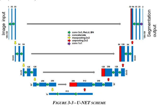
The introduction of U-NET, into the research world, came with the publication of the paper ‘U-Net: Convolutional Networks for Biomedical Image Segmentation’ [42] in which researchers from Cornell present their new type of CNN to solve segmentation problems.
Segmentation problem refers to the difficulty in identifying the regions of interest inside an image, as a tumour could be in an MRI image. Detection of high importance areas are a key step in identifying disease origins in biomedical imaging. After the detection, the area can be highlighted on the image or isolated so doctors can study the case with more ease.
The aspects that most characterize U-NET are:
1. The U-shape, that also gives the name to the model. 2. The concatenation layers.
30
The U-shape is given by its scheme representation, where are also visible its concatenation layers (GRAY arrows):
FIGURE 3-3-U-NET SCHEME
Figure above shows the U-NET first restricts the image dimension with pooling layers and augments the features by using more and more filters for every CNN layer stage, until it comes to a minimum image dimension, then it uses up-sampling to reconstruct the original image dimension following the very same scheme it has already used but in a reverse fashion and with concatenation layers. This trend, when represented, using vertical image length proportional to the image dimension and horizontal length proportional to the number of features, shows the typical U shape.
The concatenation layer brings the left element (BLUE) and concatenates it, without overlapping, with the right element (BLUE) to create one bigger element that is represented as a RED and a BLUE rectangle, corresponding to the left-moved-to-right element and to the right element, respectively. Both the samples that are concatenated have the same dimension but not the same number of features.
U-NET was born as a special adapted NN for data segmentation that could work with few instances for training, giving the possibility to train a deep model even if the dataset is rather small. Having a small dataset is a common problem when dealing with medical images because usually data are reserved and are non-homogeneous.
31
In LOUPE a slightly modified version of the U-NET is used: the core remains the very same, but a layer that computes an addition between the ‘pixelwise L2 norm of the input’ and the output of the U-NET is added to compute the output. The equation turns out to be: 𝑥̂ = 𝑈𝑁𝐸𝑇(𝐹𝐻𝑦) + ‖𝐹𝐻𝑦‖𝑝𝑖𝑥𝑒𝑙𝑤𝑖𝑠𝑒
𝐿2 = 𝐴𝜃(𝐹
𝐻𝑦).
Another difference is the input image dimension that has two channels instead of one. U-NET must consider the real and the imaginary parts of the input 𝐹𝐻𝑦 = ℝ + 𝑖 ∗ 𝕀 by using one channel for ℝ-valued elements and one for the 𝕀-valued ones.
FIGURE 3-4-U-NET USED IN LOUPE
3.2 Encoder: Adaptive Under-Sampling
The ENCODER is the part of the autoencoder that compresses the signal and, being adaptive, learns how to do it in the best way by keeping the elements with more information and discarding the others.
In first analysis, the encoder mimics the MRI data acquisition reproducing the same images that the MRI would return after its scans. The input of the ENCODER is the ground truth image 𝑥 and its output is the under-sampled image 𝑦.
More in details, the encoder is not only a module that mimics the MRI acquisition, but it adapts the MRI acquisition to the data it reads: it is an adaptive encoder.
32 1. FFT layer that brings the input into k-space 𝐹𝑥.
2. A part that learns and returns the under-sampling pattern 𝑀.
3. A layer that takes as input the under-sampling pattern and the k-space image to perform the under-sampling 𝑦 = 𝑢𝑛𝑑𝑒𝑟𝑠𝑎𝑚𝑝𝑙𝑖𝑛𝑔(𝑥, 𝑀).
The second part is the only one that is affected by the training, the other two are static parts. The encoder can be represented this way:
FIGURE 3-5-DECODER SCHEME
The under-sampling can easily be implemented performing an elementwise multiplication if 𝑀 is a mask of 0s and 1s having the same shape of 𝐹𝑥: 𝑦 = 𝑑𝑖𝑎𝑔(𝑀)𝐹𝑥.
𝑑𝑖𝑎𝑔(𝑀) is the way the elementwise multiplication is written, but no diagonalization is done, it is just notation.
So far, the loss function of the autoencoder can be written as:
min θ (∑‖𝐴𝜃(𝐹 𝐻𝑑𝑖𝑎𝑔(𝑀)𝐹𝑥 𝑗) − 𝑥𝑗‖𝐿 2 𝑁 𝑗=1 )
Where 𝑥𝑗 is one input image and 𝜃 contains all the parameter of the neural network.
The FFT and the ‘Under-sampling’ are standard modules, the heart of the problem lies in the ‘creation of the under-sampling pattern’ module that implements the function 𝑀 = 𝑚𝑎𝑠𝑘𝜃(𝑂).
33
LOUPE offers high flexibility when it comes to define the sparsity level of 𝑦, LOUPE offers two different implementations to realize the under-sampling pattern.
The first implementation, the one that is going to be explained in more details, defines a parameter called ‘sparsity’ (𝛼) in a range [0,1] and returns a mask 𝑀 with mean 𝛼. Being 𝑀 a mask with only 0s and 1s values and having mean 𝜇(𝑀) = 𝛼, the normalized sparsity ‖𝑀‖𝐿0
𝑑 =
𝛼, 𝑑 = 𝑛𝑢𝑚𝑏𝑒𝑟 𝑜𝑓 𝑒𝑙𝑒𝑚𝑒𝑛𝑡𝑠(𝑀), in other words the number of 1s in M #1(𝑀) = 𝛼 ∗ 𝑑 and all the other elements are null. For this reason, 𝛼, even if is not the real sparsity definition ‖⋅‖𝐿0, is called sparsity.
The other implementation does not output a mask 𝑀 with a given sparsity, but it finds the best 𝑀 given a penalty on the sparsity of 𝑀, that is added to the loss function. This method takes as input a parameter 𝜆 that defines how the sparsity constraint weights with respect to the other part of the loss function.
Both the methods require 𝑀 to be sparse, mathematically it can be called a constraint.
The first implementation is called ‘𝛼-method’, the other is called ‘constraint-method’. Now the 𝛼-method is introduced.
After the addition of the constraint of the sparsity the loss function becomes:
min θ (∑‖𝐴𝜃(𝐹 𝐻𝑑𝑖𝑎𝑔(𝑚𝑎𝑠𝑘(𝑂))𝐹𝑥 𝑗) − 𝑥𝑗‖𝐿 2 𝑁 𝑗=1 ) , 𝑠𝑢𝑐ℎ 𝑡ℎ𝑎𝑡‖𝜎𝑙(𝑂)‖𝐿1 𝑑 = 𝛼 Where ‖𝜎𝑙‖𝐿1 = 𝜇(𝑃) = 𝑚𝑒𝑎𝑛(𝑃).
The great intuition in LOUPE is to create a custom layer called ‘ProbMask’ that returns an element containing its weights. ProbMask is a simple layer that takes an input but discards it and only outputs its weights 𝑂. The weights 𝑂 of the layer are TRAINABLE and are the only weights that can be modified during training in the ENCODER.
Because the mask is trainable and 𝑂 becomes a parameter to minimize the loss function with, the loss function can be written:
min θ,O (∑ 1 𝐾∑‖𝐴𝜃(𝐹 𝐻𝑑𝑖𝑎𝑔(𝑚𝑎𝑠𝑘(𝑂)(𝑘))𝐹𝑥 𝑗) − 𝑥𝑗‖𝐿 2 𝐾 𝑘=1 𝑁 𝑗=1 ) , 𝑠𝑢𝑐ℎ 𝑡ℎ𝑎𝑡‖𝜎𝑙(𝑂)‖𝐿1 𝑑 = 𝛼
34
𝑚𝑎𝑠𝑘(𝑂)(𝑘) represents an instance of 𝑀, to find the best possible 𝑀 is necessary to test over many masks (𝐾). 𝑚𝑎𝑠𝑘(𝑂)(𝑘) are independent realizations of a random process that generates the masks: this is a smart way to introduce randomness and to secure the mask is well-trained. 𝑂 is the first and most important element of the block that adapts itself to be minimize the loss function, the remaining layers transform 𝑂 into 𝑀 by the addition of some requirements, these are the steps:
1. Bring values of 𝑂 from ℝ to (0,1). 2. Initialize O.
3. Apply the 𝛼 sparsity.
4. Introduce the randomness in the process to create 𝑀. 5. Adapt the procedure to be ‘trainable’.
The first point is easy to satisfy: a ‘sigmoid’ function 𝜎 can be applied: 𝑃 = 𝜎𝑙(𝑂).
FIGURE 3-6-SIGMOID FUNCTION
Figure above contains the plot of a standard sigmoid with 𝑙 = 1. In general, 𝜎𝑙(𝑧) = 1
1+𝑒−𝑙∗𝑧,
where a higher 𝑙 means a steeper sigmoid, as 𝑙 rises 𝜎𝑙 tends to resemble a hard threshold. In a Dense layer as usually happens, 𝑧 is assumed to be the typical output of a neuron 𝑧 = ∑𝑤𝑖𝑥𝑖 + 𝑏𝑖𝑎𝑠 and the sigmoid is its activation function, in the ProbMask case the only
35
Sigmoid function brought 𝑂 from ℝ to a continuous range of values [0,1]. Is important to initialize 𝑃 with well distributed elements to help the training converge during the first epochs. Because sigmoid is not linear the initialization of 𝑂 must return the desired distribution once sigmoid is applied. In LOUPE has been found that a good start is provided by 𝑂0 = ln ( 𝑥
1−𝑥) 1 𝑙 ,
𝑔𝑖𝑣𝑒𝑛 𝑥 ∼ 𝑈(ξ, 1 − 𝜉), 𝜉 𝑠𝑚𝑎𝑙𝑙 ∼ 0.01. The final distribution of 𝑃 is 𝑃0 = 1 − 𝑥.
The 𝛼-implementation deals with the constraint ‖𝜎𝑙(𝑂)‖𝐿1
𝑑 = 𝛼, defining a function 𝑁𝛼.
To obtain the final desired sparsity 𝛼 in 𝑀, 𝑃 needs to have mean of 𝑃 equal to 𝜇(𝑃) = 𝛼. The custom layer ‘RescaleProbMask’ in LOUPE achieves this step by rescaling: 𝑃𝛼= 𝑁𝛼(𝑃). The new function 𝑁𝛼 is:
𝑃𝛼= {
𝛼
𝜇(𝑃)∗ 𝑃, 𝑖𝑓 𝜇(𝑃) ≥ 𝛼 1 − 1 − 𝛼
1 − 𝜇(𝑃)∗ (1 − 𝑃), 𝑜𝑡ℎ𝑒𝑟𝑤𝑖𝑠𝑒
𝑁𝛼 turns the mean 𝜇(𝑃) = 𝛼, this way ensures the constraint is satisfied and the loss function
does not need it to be specified as an explicit constraint anymore. 𝑁𝛼 turns an explicit constraint into an implicit one.
To implement the randomness into the scheme, LOUPE inserts two special layers called ‘RandomMask’ and ‘ThresholdRandomMask’ respectively.
The first layer creates a matrix 𝑈 with the same dimension of 𝑃. Every element of 𝑈 is a random uniform distributed value in the range [0,1]: 𝑈 ∼ 𝑈(0,1). This layer takes no inputs.
The output of RandomMask is passed to ThresholdRandomMask that takes as input also 𝑃 and computes the hard threshold 𝑀 = 𝑃𝛼 > 𝑈. It returns a matrix of 0s and 1s that is used as
under-sampling mask. In the location where 𝑃𝛼> 𝑈 the element of 𝐹𝑥 will be taken, otherwise it will be discarded.
At this point many steps can be compressed together and inserted into the loss function:
min θ,O (∑ 1 𝐾∑‖𝐴𝜃(𝐹 𝐻𝑑𝑖𝑎𝑔(𝑁 𝛼(𝜎𝑙(𝑂)) > 𝑈(𝑘))𝐹𝑥𝑗) − 𝑥𝑗‖𝐿 2 𝐾 𝑘=1 𝑁 𝑗=1 )
Because now the randomness of 𝑀 has been lifted to the random generation of 𝑈, it is 𝑈 that acquires the ⋅(𝑘) to explicit that the mask is adapted over 𝐾 generation of 𝑈.
36
As it seems everything is done such that both the encoder and the decoder have been completed, there is still one more adjustment to do: the function as it is written is not trainable. During training is necessary to have all differentiable functions, otherwise backpropagation cannot compute the gradient and cannot work. Inside the loss function the part (𝑁𝛼(𝜎𝑙(𝑀)) > 𝑈(𝑘))
is not differentiable.
To solve this problem is necessary to lighten the assumption that the mask is a binary matrix. As long as 𝑀 lives into a discrete space it cannot be derivable, the solution is obviously to let elements in 𝑀 belong to the continuous range [0,1]. LOUPE solves the problem using a difference instead of greater operation and to bring back in the [0,1] domain the outcome it uses a sigmoid 𝜎𝑠 with a high steepness (high 𝑠) to mimic the threshold but remaining continuous. Mathematically 𝑀 = 𝜎𝑠(𝑁𝛼(𝜎𝑙(𝑀)) − 𝑈(𝑘)).
The loss function is updated to:
min θ,O (∑ 1 𝐾∑ ‖𝐴𝜃(𝐹 𝐻𝑑𝑖𝑎𝑔 (𝜎 𝑠(𝑁𝛼(𝜎𝑙(𝑂)) − 𝑈(𝑘))) 𝐹𝑥𝑗) − 𝑥𝑗‖ 𝐿2 𝐾 𝑘=1 𝑁 𝑗=1 )
One last consideration: 𝐾 in LOUPE is set to 𝐾 = 1 because, as reported in [40], it is a computationally efficient approach that yields an unbiased estimate of the gradient that is used in stochastic gradient descent. The loss function finally is simplified to:
min θ,O (∑ (‖𝐴𝜃(𝐹 𝐻𝑑𝑖𝑎𝑔 (𝜎 𝑠(𝑁𝛼(𝜎𝑙(𝑂)) − 𝑈(𝑘))) 𝐹𝑥𝑗) − 𝑥𝑗‖ 𝐿2 ) 𝑁 𝑗=1 )
The second implementation, called ‘regularization-method’, instead of defining a parameter 𝛼 to force the desired sparsity of 𝑀, defined a regularization parameter 𝜆 to control the weigh of a regularization factor added to the loss function.
This method is based on many of the considerations that have been done for the 𝛼-method. All the layers are the same, expect for RescaleProbMask that is missing. Because RescaleProbMask is not used, in the loss function the formula 𝑁𝛼 is missing and the sparsity task is carried by the
regularization function 𝜆 ∗ ‖𝑀(𝑘)‖
𝐿1. The 𝐿1 norm of 𝑀 is minimized leading to a higher
37 min θ,O (∑ (‖𝐴𝜃(𝐹 𝐻𝑑𝑖𝑎𝑔 (𝜎 𝑠(𝜎𝑙(𝑂) − 𝑈(𝑘))) 𝐹𝑥𝑗) − 𝑥𝑗‖ 𝐿2 ) 𝑁 𝑗=1 + 𝜆 ∗ ‖𝑀(𝑘)‖𝐿 1)
This method guarantees the mask sparsity, but do not guarantees for a specific value of sparsity. This makes the method not as competitive as the 𝛼-method and will not be discussed anymore.
3.3 Autoencoder
From the loss function evident how the approach of LOUPE tackles the two main aspects of CS together:
1. The encoder finds the best under-sampling pattern by training the ProbMask layer and modifying 𝑂.
2. The decoder adapts to obtain the best possible reconstruction by modifying the weights 𝜃 of the U-NET.
The heart of LOUPE is in its double simultaneous adaptiveness. Not only the reconstruction can adapt to the under-sampled image, but the under-sample pattern can adapt itself to the reconstruction.
The implementation of LOUPE can be represented showing its layers:
FIGURE 3-7-LAYERS OF LOUPE
The representation shows all the layers of the encoder, for the decoder the U-NET has been represented as a unique layer, even if as already explained it composed by many different layers.
38
An important aspect of LOUPE that in the Figure below is highlighted are its trainable and non-trainable parts. It is clear from the figure that for building an adaptive encoder only ProbMask needs to be trainable, and for building the decoder only the U-NET needs trainable parameters. A more detailed representation that shows more mathematical relationships:
FIGURE 3-8-LAYERS OF LOUPE WITH FORMULAS
3.4 Results and conclusions
The study [40] trained LOUPE on knee MRI dataset. In particular the considered dataset is the ‘NYU fastMRI’ dataset [43] (fastmri.med.nyu.edu). [43] is a freely available, large-scale, public set of knee MRI scans.
Validation functions such as MSE, MAE, PSNR, SSIM and HFEN [44] were used to evaluate the results.
More in details the validation function are defined as:
𝑃𝑆𝑁𝑅(𝑥, 𝑥̂) = 10 ∗ 10 log ((max(𝑥))
2𝑑
‖𝑥 − 𝑥̂‖22 )
SSIM(x, 𝑥̂) = (2μxμx̂+ c1) + (2σ𝑥𝑥̂ + c2) (μ𝑥2 + μ𝑥̂2 + c1)(σx2+ σ𝑥̂2 + c2)
Parameter definition has been provided in [40].
LOUPE has been compared to three different non-ML benchmarks and with one ML benchmark: the three non-ML are BM3D [45], LORAKS [18], TGV [46], the ML one is a U-NET. Every model does not adapt to find the best sampling patter but receives under-sampled MRI images whom under-sampling patter was not trained but was user-defined.
39
The used pattern (for the benchmarks) are Random Uniform pattern [47], [48], parametric variable density [49], [50], data-driven strategy [51], cartesian [52] and line constraint [53]. LOUPE has shown good performances with respect to the other methods, classifying as a novel and functional approach for implementing CS MRI acquisitions.
Based on the ‘NYU fastMRI’ dataset [43] and on acceleration rates 4 and 8 (corresponding to 𝛼 𝑖𝑛 [0.25, 0.125]) LOUPE scored:
40
41
As it is possible to see from the Figure above LOUPE scored always better than the other methods. Figure below shows an example of reconstruction using LOUPE, the dataset consists of knee MRI scans. The image has been taken from [40].
FIGURE 3-10LOUPE EXAMPLE OF RECONSTRUCTION
3.5 Problems and how to improve LOUPE.
Even if LOUPE is a competitive and well-structured method it still has potentialities to exploit farther.
42
1. Regarding the loss function, when the operation 𝑃𝛼 > 𝑈(𝑘) is modified into 𝜎𝑠(𝑃𝛼− 𝑈(𝑘)) the original threshold function is approximated into a sigmoid. This approximation must be tuned via the tuning of the slope 𝑠 of the sigmoid 𝜎𝑠. The tuning of 𝑠 can be skipped by the gradual and constant increasing of 𝑠 during training.
2. The training can be aided by requesting the reconstructed image 𝑥̂ to have the same known frequency components of 𝑦, ensuring that the reconstruction process does not warp the components that are known to be correct.
3. An indicator of the reconstruction success can be found comparing the frequency components of 𝑥̂ with the known frequency components of 𝑦. This result can be used, after training, as a detector for reconstruction failures, or as an indicator that points out if the training is successful or not.
4. In LOUPE, before the under-sampled data 𝑦 is given as input to the U-NET, 𝑦 is moved from k-space to Euclidian space using the IFFT: 𝐹𝐻𝑦. This step can be generalized by
the use of a LOUPE-learned transformation.
All these points are ideas to improve LOUPE working on details, that do not modify the kernel of it.
In the next chapter some contributions to LOUPE will be explained and justified, showing in detail how they work and how they improve LOUPE.