Analysis of landslides reactivated by variation in the groundwater regime

(1)

UNIVERSITA’ DELLA CALABRIA

ANALYSIS OF LANDSLIDES REACTIVATED BY VARIATION IN THE GROUNDWATER REGIME

Ph.D. DISSERTATION BY

ANTONIO DONATO

Ph.D. school in Geotechnical Engineering Mediterranean University of Reggio Calabria

Department of Civil Engineering University of Calabria

(2)

By

ANTONIO DONATO Ph.D. Candidate

Ph.D. school in Geotechnical Engineering (XXVII cycle) Mediterranean University of Reggio Calabria

SUPERVISORS Professor E. Conte _____________________________________ Professor A.Troncone _____________________________________ COORDINATOR Professor N. Moraci _____________________________________

(3)

I Landslides can cause considerable damages to infrastructures and human lives. These phenomena appear in different kinematic forms: from extremely slow to extremely rapid. Although slow-moving slope movements do not frequently cause loss of human lives, they may damage structures, interrupt lifelines (highways, railways, pipelines) and require very high costs for their stabilisation. The aim of this research is to propose some approaches for the analysis of landslides controlled by changes in the pore pressure within the slope. In the first part, slow-moving landslides are analyzed. These landslides are characterized by the evidence that deformations are mostly concentrated within a narrow shear zone above which the unstable soil mass essentially moves as a rigid body. Two different approaches are proposed: the first one is a simplified method that is based on the infinite slope model to assess slope stability and on some analytical solutions to predict landslide mobility. The second one utilises a finite element approach in which an elasto-viscoplastic constitutive model in conjunction with a Mohr-Coulomb yield function is incorporated to describe the behaviour of the soil in the shear zone.

For the other soils involved by the landslide, an elastic model is used for the sake of simplicity. A significant advantage of the present methods lies in the fact that few constitutive parameters are required as input data, the most of which can be readily obtained by conventional geotechnical tests.

(4)

II the associated movements of the unstable soil mass. After being calibrated and validated, both approaches can be used to predict future landslide movements owing to expected groundwater fluctuations or to assess the effectiveness of drainage systems which are designed to control the landslide mobility.

These methods are applied to back-predict the observed field behaviour of three active slow-moving landslides documented in the literature. In the second part of the work, a landslide of large dimensions (about 6 million of cubic meters) that occurred in Maierato (Calabria) on 2010, after a long period of heavy rainfall is analyzed using a finite element approach in order to establish the main causes of the landslide event and to define the failure process occurred.

(5)

III

Acknowledgements

This work has been carried out under the supervision of Professors Enrico Conte and Antonello Troncone in Geotechnical Engineering of Civil Engineering Department in University of Calabria.

The author wishes to express his sincere appreciation to supervisors for their advices and guidance during all time of this research.

Furthermore, the author extends heartfelt thanks to his “brothers in arms” Mirko Vena, Andrea Chidichimo and Paolo Zimmaro for their moral and professional support, which has been always useful.

The author will be always grateful to his family and Caterina for their tireless encouragement and infinite patience.

(6)

IV

Introduction

The present work concerns the analysis of active landslides which are controlled by changes in the pore water pressure regime within the slope. Usually, these landslide occur in gentle slopes of clayey soils. The main type of movement experienced by them is a translational or roto-translational slide with a velocity of order a few centimetres per year. Therefore, they can be classified as very slow or extremely slow landslides, according to Cruden and Varnes (1996). Typically, deformations are concentrated within a shear zone located at the base of the landslide body, in which the soil shear strength is at residual conditions owing to the high level of accumulated strain (Leroueil et al., 1996). The landslide body on the contrary experiences very small strains, so that it essentially moves as a rigid body. Generally, the slope movements are caused by an increase in pore water pressure with the total stress field that remains practically unchanged with movement. This increase in pore pressure determines a decrease in the effective stress level and consequently in the soil shear strength along the slip surface. Considering that the slope safety factor,

SF, is governed by the residual strength along the slip surface, the values of SF

are generally low. Therefore, small changes in pore pressure can produce significant changes in the displacement rate of the unstable soil mass. These changes are often caused by groundwater level fluctuations which in turn are related to rainfall. Therefore, the mobility of these landslides is characterized by alternating phases of rest and reactivation in accordance with the seasonal

(9)

2 rainfall conditions. In particular, raising of the groundwater level causes a reactivation and subsequent acceleration of the landslide because the resisting force decreases and cannot balance the destabilising force. On the other hand, a groundwater level reduction (as occurs during dry periods) mitigates the landslide velocity and may eventually bring the soil mass to rest. The continuous reactivation phases can cause significant damage to the structures and infrastructures located on the slope. Therefore, an adequate consideration of these phenomena is necessary for performing realistic slope stability analyses. In the current applications, groundwater pressure regime and slope stability are usually dealt with in an uncoupled manner using some theoretical approaches. Specifically, the differential equations governing pore pressure changes within the slope due to changes in hydraulic conditions at the boundary are first solved. Then, the pore pressures calculated at the potential failure surface are used in a limit equilibrium analysis for assessing slope stability.

Simplified methods were also developed to perform directly an approximate assessment of the landslide velocity (Angeli et al., 1996; Gottardi and Butterfield, 2001; Corominas et al., 2005; Maugeri et al., 2006; Herrera et al., 2009; Conte and Troncone, 2012a). In these methods, it is assumed that the landslide body behaves as a rigid block sliding on an inclined plane.

Numerical models based on the finite element method or the finite difference method, in which reliable constitutive laws are incorporated, can provide a better understanding of the complex mechanisms of deformation and failure that occur in the slope.

(10)

3 In this work, active landslides are analysed using two approaches: a simplified method proposed by Conte & Troncone (2011) utilises an analytical solution and assumes that the landslide body behaves as a rigid block sliding on an inclined plane, and the finite element method. In this latter approach, an elasto-viscoplastic constitutive model is included to predict the behaviour of the soil in a finite shear zone located between the moving mass and the underlying stable geological formation. Both the proposed approaches are applied to assess the mobility of well documented active landslides which are periodically activated owing to groundwater level fluctuations. Lastly, a landslide of large dimensions that occurred in Calabria after a long period of heavy rainfall is analysed using a finite element approach in order to study the failure process observed.

The thesis is organized in four chapters: in the first one is reported a literature review concerning landslides caused by changes in the pore water pressure regime. In the second chapter is shown a detailed description of the proposed methods, which are afterwards applied in the third chapter to three active landslides. Finally, the last chapter reports an extensive study on the landslide occurred in Maierato (Southern Italy) on 15 February 2010. This study includes a description of the area, geological and geotechnical characteristics of the soils involved along with an analysis of documents and videos caught by local people, which have provided important information on the failure process occurred. Finally, the numerical analyses have shown that the landslide was a reactivation caused by a considerable increase in the pore water pressure owing to rainfall.

(11)

4

Chapter 1 Landslides induced by pore water

pressure changes

1.1. Movements and failure mechanisms of natural slopes

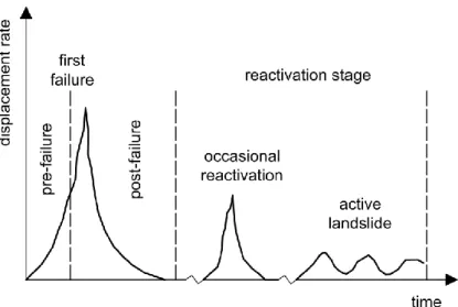
Movements of slopes are a complex problem that involves a variety of geomaterials in different geological and climatic contexts. In order to simplify their analysis, Vaunat et al. (1994) and Leroueil et al. (1996) suggested classifying slope movements into four stages, as listed below and illustrated in Fig.1.1:

1. Pre-failure: this stage includes all the deformation processes leading to failure due to changes in stresses, creep and progressive failure.

2. Failure: characterized by the formation of a complete shear zone through the whole soil mass.

3. Post-failure: it includes landslide movement just from after the onset failure until it stops.

4. Reactivation: the unstable soil mass slides on a pre-existing shear surfaces along which the residual shear strength is at residual condition.

(12)

5 Fig. 1.1 – Schematic evolution of displacement rate (modified from Leroueil, 2001)

Fig.1.2 shows a possible time-horizontal displacement relationship for each stage above-mentioned (Picarelli, 2000).

Fig. 1.2 –Evolution of the horizontal displacement of a point located on the failure surface (Picarelli, 2000)

As it can be seen, the reactivation stage is generally characterized by alternate phases of rest and motion. Movements are caused by a reduction of the soil shear strength along the existing slip surface, for example owing to changes in the pore water pressure regime induced by rainfall.

(13)

6

1.2. Rainfall-induced slope failures

Basically, slope failure due to rainfall is mainly caused by: 1. increase in weight of the soil mass;

2. decrease in suction for unsaturated soils owing to water infiltration; 3. rise in groundwater level.

Fig.1.3. shows a flowchart which illustrates the mechanism of rainfall-induced slope failure. Rainfall causes an increase in pore water pressure and consequently a reduction of the soil shear strength which can lead to slope failure.

Fig. 1.3 – Mechanism of rainfall-induced slope failure

A shallow landslide usually occurs in the unsaturated zone of the soil. Also, groundwater table goes up causing deformation of soil mass up to the occurrence of slope failure. In this case, the slip surface is generally deep and develops mostly in the saturated zone of the soil.

(14)

7 1.2.1. Slope failure in unsaturated conditions

Due to rainfall infiltration, suction and consequently the soil shear strength decrease. According to the following equation proposed by Fredlund (2000):







  

_f c u_a tan  stan  (1.1) in which τf =failure shear stress, c' = effective cohesion, =shear strength angle

of the soil, σ = total normal stress; ua = pore air pressure, s= matrix suction

(s=ua-uw, in which uw = pore water pressure), and χ = parameter ranging from 0

to 1. The following expression may be employed for χ (Fredlund et al., 1996):

      _         r s r _(1.2)

in which θ = volumetric water content at a given suction, θs = volumetric water

content at saturation, θr = residual volumetric water content, λ = a fitting

parameter depending on the soil type. As suggested by Fredlund (2000), a value of λ = 1 may be assumed for most inactive soils, such as sand, silt and some fine-grained soils in the suction range of 0-500 kPa. In this case χ can be therefore obtained directly from the soil-water characteristic curve of the soil as a function of suction.

(15)

8 Infiltration process in unsaturated soils represents a complex problem to be analyzed. In particular, it needs to take into account:

 initial conditions (pore pressure in function of the antecedent hydrologic events);

 degree of saturation, matrix suction and hydraulic conductivity.

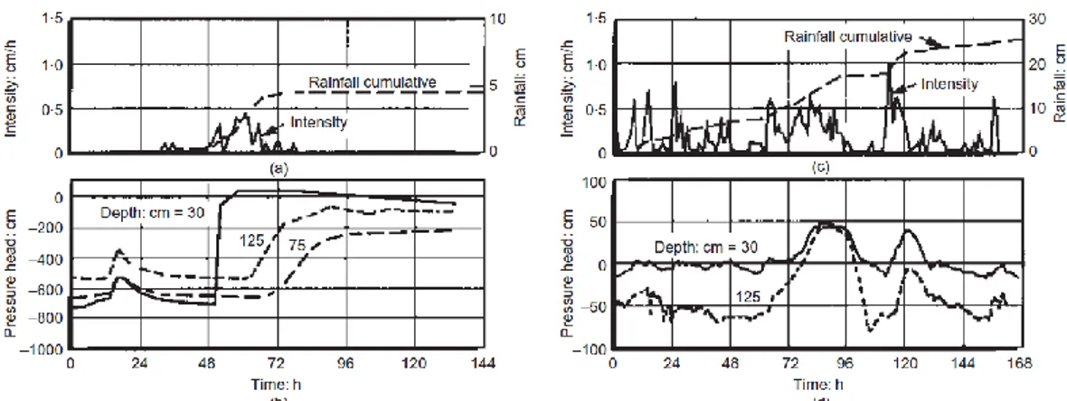
Several theoretical and numerical studies (Alonso et al., 1995; Collins & Znidarcic, 1997; Sun et al., 1998) were carried out in order to analyze water infiltration in unsaturated soils. Pore pressure measurements performed using piezometers and tensiometers installed in a thick layer of residual soils outcropping in the Sila Massif in Italy were presented by Gullà & Sorbino (1996). In particular, Fig. 1.5 shows some periods during which pore pressure in the shallowest tensiometer (at a depth of 0.81 m) remain essentially constant, although rainfall was close to the maximum value measured during the observation period. This indicates that the wetting front did not propagate to at depth and that it is also necessary to consider evapotranspiration and runoff (from Leroueil, 2001).

(16)

9 Fig. 1.5–Daily rainfall and pore pressure measurements at Sila Massif (Gullà & Sorbino, 1996)

Similar measurements were made by Johnson & Sitar (1990) in the Briones Regional Park, close to San Francisco. The authors report the pore pressure measurements during the rainfall events on 24 November 1985 and 12-20 February 1986 (Fig.1.6). Pore pressure response to rainfall was quick at the shallowest depth and gradually propagated with delay (12-24 hours) at larger depth. Furthermore, this study evidences the influence of the antecedent conditions on pore pressure response to rainfall.

(17)

10 Fig. 1.6–Rainfall and pore pressure measurements at Briones Hills (Johnson & Sitar, 1990)

Observations made by Lacerda (1989), Johnson & Sitar (1990), Montgomery et al. (1997) showed that the development of pore pressure and the failure in unsaturated condition may not result from vertical infiltration only, but also from flows of water through more permeable soil layers and fractured bedrock. Water flow into slopes may also be influenced by animal burrows, desiccation cracks and root holes. The hydrologic and hydrogeological response of a hillslope to rainfall may thus be complex, as schematized in Fig. 1.7, and complicates the prediction of failure.

Fig. 1.7– Scheme of the hillslope hydrologic response to rainfall; arrows indicate groundwater flow directions (after Lacerda, 1989; Johnson & Sitar, 1990)

(18)

11 1.2.2. Slope failure in saturated conditions

Landslides are caused by an increase in groundwater level and the failure surface mostly develops within the saturated zone of the soil. Generally, these landslides are denoted as active landslides. Active landslides are often controlled by the groundwater level fluctuations which in turn are related to rainfall. The mobility of these landslides is characterized by alternate phases of rest and reactivation according to the weather conditions. In particular, a rising groundwater level owing to rainfall can cause a reactivation of the landslide or, if it is moving, an acceleration of the motion. On the other hand, a groundwater level reduction (as it occurs during dry periods) attenuates the landslide velocity and can bring the unstable soil mass to rest. The main type of movement experienced by these landslides is a translational or roto-translational slide with a velocity of order of some centimetres per year, so that they can be defined as slow-moving landslides (Cruden and Varnes, 1996). Generally, deformations are concentrated within a shear zone located at the base of the landslide body, in which the soil shear strength is at residual condition owing to the high strains accumulated (Leroueil et al., 1996). The soil above the shear zone is on the contrary affected by very small strains and it is characterized by a horizontal displacement profile that is essentially constant with depth.

(19)

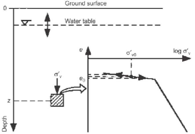
12 A change in pore pressure at a certain depth produces a change in effective stress, and consequently, in void ratio. For one-dimensional conditions, this is illustrated in Fig. 1.9.

Fig. 1.9– Changes in void ratio due to changes in pore pressure condition for compressible material (from Leroueil, 2001)

Swelling/consolidation process for two-dimensional conditions and isotropic hydraulic conductivities (kx=kz) is controlled by Eq. (1.3).

                          2 2 2 2 2 2 2 2 z u x u c z u x u m k t u _w _w v w w w w  (1.3)

where t is time, x and z are spatial coordinates, k is the hydraulic conductivity,

m denotes the coefficient of volume change and cv is the swelling/consolidation

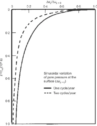
coefficient of the soil. As a result of this process, the seasonal variation of pore pressure at upper and lower boundaries of saturated soil deposit is not entirely reflected inside it. Specially in clayey deposits, the upper part is often fissured and behaves as an open aquifer in which water level varies by a maximum amount corresponding to Δuz=0 (amplitude of pore pressure variation at the

ground surface). Fig. 1.10 shows the relative amplitude of pore pressure (Δuz/Δuz=0), in which Δuz is the amplitude of pore pressure variation at a depth

(20)

13

z, as a function of z2/cv for a sinusoidal variation of the pore pressure at the

boundary (solution given by Carlslaw & Jaeger,1959). The soil deposit is assumed saturated and semi-infinite, bounded by a horizontal surface. In particular, two curves are shown: the continuous curve corresponds to one sinusoidal cycle per year, whereas the other is relative to two sinusoidal cycles per year. An analytical solution for analysing this process under more general boundary conditions, was derived by Conte & Troncone (2008).

Fig. 1.10 – Variation of pore pressure in a soil deposit due to a sinusoidal variation of pore pressure at the surface (from Leroueil, 2001)

(21)

14

1.3. Landslide mobility owing to seasonal variations of pore

water pressure

Active landslides which are controlled by groundwater fluctuations typically occur in gentle slopes of clayey soils and are characterized by a velocity of order of some centimetres per year. In this regard, IUGS (1995) and Cruden & Varnes (1996) proposed a classification based on the values of the landslide velocity. In particular, seven different classes were defined in Tab.1.1.

Class Description Typical velocity limits (mm/day)

1 Extremely slow < 4.4·10-2 (<16mm/year)

2 Very slow 4.4·10-2 - 4 3 Slow 4 - 433 4 Moderate 433 - 4.3·104 5 Rapid 4.3·104 - 4.3·106 6 Very rapid 4.3·106 - 4.3·108 7 Extremely rapid > 4.3·108 (>5m/s)

Tab. 1.1 – Classification proposed by IUGS, 1995 and Cruden & Varnes, 1996

Therefore, the landslides at issue typically fall into classes 1 to 3. Analysis, modeling and prediction of such phenomena present several difficulties, essentially attributable to four different sources (Vulliet & Hutter, 1988c):

 most movements occur in isolated and remote areas and access to the sites may be difficult;

 monitoring of slow movements (typically few centimeters per year) needs a large period of observation;

 modelling the time-dependent behaviour of the soils involved requires specific tests and adequate constitutive models.

 slope movements are strongly affected by hydrological factors.

In spite of these difficulties, a remarkable improvement has been made in the last years. Theoretically, movements start at the beginning of rainy season and stop during dry season when rain infiltration is poor. It is possible to establish a

(22)

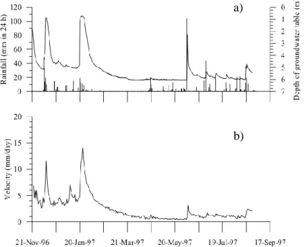
15 triggering threshold, represented by a critical value of pore pressure beyond which a reactivated landslide occurs. Nevertheless, the real behaviour of the soils is essentially viscous and slopes may move even if rainfall is zero. As an example, the relationship among rainfall, groundwater level and velocity of the Vallcebre landslide are shown in Fig.1.11 (Corominas et al., 2000). It is worth noting that in some periods the landslide moves, although rainfall is nil.

Fig. 1.11 – a): rainfall records (bars) and groundwater level changes at a borehole. b): velocity of landslide at the same borehole (Corominas et al., 2000)

Two factors should be considered for analyzing active landslides: the viscous behaviour of the soils involved and the shear strength along the pre-existing slip surface that is at residual condition.

a)

(23)

16 1.3.1. Residual shear strength

The residual strength assumes great importance in analyzing slope stability. In particular, it is reached after large displacements when a parallel reorientation of platy to shearing direction is achieved. Residual strength is influenced by several factors, such as mineralogy, shape of particles, normal stress, type of shearing, pore pressure and rate of displacement.

Fig. 1.12 – Brittleness of soils (modified from Leroueil, 2001)

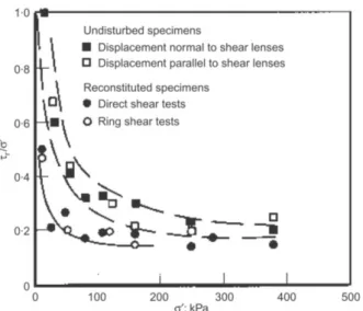
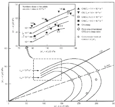
For many clayey soils, the relation between normal effective stress and residual strength is nonlinear (Skempton, 1985; Stark & Eid, 1994). A typical example is shown in Fig. 1.13, which reports some experimental results of laboratory tests on reconstituted specimens of Laviano clay (Picarelli, 1991).

(24)

17 Generally, the soil consists of both round and platy particles. In this connection, Lupini et al. (1981) presented the results in Fig. 1.14, from which it is evident that if the percentage of platy particles is small, no reorientation of them (rolling shear) is observed. Therefore, the residual shear angle  'r is slightly smaller than that at the critical state,  'cr. Conversely, if the percentage of platy particles is large, a reorientation of them is observed. The residual shear angle

'r is significantly smaller than that corresponding to the critical state, 'cr.

Fig. 1.14 – Ring shear tests on sand-bentonite mixtures (Lupini et al., 1981; Skempton, 1985)

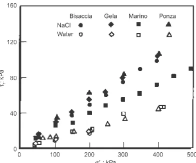
The residual strength increases by a few percent when the rate of displacement increases by one order of magnitude. This is not significant when slope stability is analyzed (Skempton, 1985), but it assumes remarkable consequences for the movements at each reactivation stage. Important effects on the residual shear angle can be ascribed to pore water chemistry (Di Maio, 1996 a,b). In particular, Fig. 1.15 shows some results obtained on three Italian clays and on Ponza bentonite. The specimens were prepared either with saturated NaCl solution or with distilled water.

(25)

18 Fig. 1.15 - Residual shear strength plotted against normal stress of specimens reconstituted with

water and specimens reconstituted with saturated NaCl solution (Di Maio, 1996a)

As it can be seen, saturating the specimens with NaCl solution leads to higher values of  'r. Furthermore, 'r also varies with the concentration of NaCl solution, as shown in Fig. 1.16. As it can be seen, significant changes in ’r occur for concentration of NaCl between 0 and 35 g/l.

(26)

19 1.3.2. Viscous behaviour of the soil

Landslide movements can be delayed due to pore pressure redistribution (D’Elia et al., 1985) or viscous effects (Bracegirdle et al., 1992; Savage and Chleborad, 1982; Vulliet and Hutter, 1988; Van Asch and Van Genuchten, 1990; Leroueil and Marques, 1996). Owing to viscous nature of the soils, the velocity may not abruptly vary even if the safety factor tends to unity. The rate of displacement, v, depends on the shear stress, τ, along the slip surface according to the following relationship:



f

v



(1.4)

where f is a function related to viscosity, soil strength and stress acting on slip surface. Evidence of the viscous behaviour of the clayey soils was observed in several tests. The behaviour observed in creep tests can be described by the following equation (Singh & Mitchell, 1968):

m t t q Ae _        1 1   (1.5)

where ₁represents the axial strain rate, t the time, q is the stress ratio (equal to the applied deviatoric stress divided by the deviatoric stress at failure for conventional compression tests), m is the slope of log₁-log t curve, t1 is a

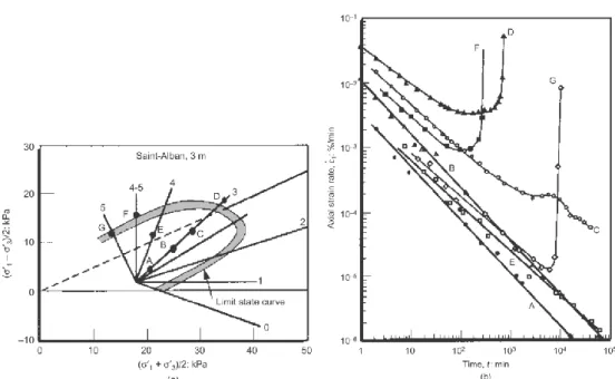
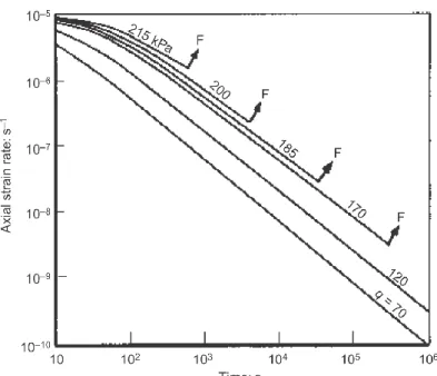
reference time generally equal to 1 min, and α and A are creep parameters. Bishop & Lovenbury (1969), Larsson (1977), Tavenas et al. (1978), and D’Elia (1991) performed long-term creep tests on clayey soils. In particular, Fig. 1.17 shows the creep test results obtained on Saint Alban clay, for different stress conditions inside the limit state curve.

(27)

20 Fig. 1.17 – Axial strain rate vs. time for creep tests on Saint Alban clay (Tavenas et al., 1978)

The results in Fig.1.17b show the development of creep strains with time along linear relationships in a logarithm diagram of axial strain rate versus time. Considering the points D, F, G, the strain rate increases up to failure after reaching a minimum value. Similar results were achieved for the Santa Barbara clay (D’Elia, 1994) and on some shale clays (D’Elia, 1991), as shown in Fig. 1.18.

Fig. 1.18 – Axial strain rate vs. time for creep tests at various stress levels (q/qf) on:

(28)

21 Fig. 1.19 shows the results of the tests performed on the stiff Mascouche clay by Marchand (1982). The stress conditions referred to failure are indicated with square and triangle symbols. Long-term triaxial creep tests are also carried out with stress conditions marked as black dots.

Fig. 1.19 – Influence of strain rate on the limit state curve of Mascouche clay (Leroueil & Marques, 1996 after Marchand, 1982)

Other creep tests were performed with different deviatoric stress (Figs. 1.20-1.22). Also in these tests the behaviour of soil presents strain rate dependence.

Fig. 1.20 – Strain rate dependence of stress-strain behaviour and input parameters of triaxial creep tests simulation (Leroueil, 1998a)

(29)

22 Fig. 1.21 – Simulated creep tests for the conditions from Fig.1.20 (Leroueil, 1998a)

Fig. 1.22– Simulated creep tests in which the deviatoric stress is 190 kPa for 3000 min and then decrease to 170 kPa (Leroueil, 1998a)

The critical accumulated strain seems to assume an important role, because after a slight decrease in deviatoric stress (from 190 to 170 kPa after 50 min), creep strain continues to develop until the soil reaches failure.

(30)

23

1.4. From hydrologic conditions to landslide mobility

An important objective for the geotechnical engineers is to establish a relationship for practical use among hydrologic conditions, pore pressure, soil strength, safety factor and rate of movement. Fig.1.23 shows the conceptual scheme proposed by Leroueil (2001) to illustrate the possible approaches that can be used to relate rainfall to landslide mobility. According to Fig. 1.23, the most complete approaches start from rainfall and include all the intermediate steps, such as pore pressure changes, soil strength and safety factor, and finally rate of movement.

Fig. 1.23 - From hydrologic conditions to safety factor and rate of displacement (modified after Leroueil, 2001)

In the current applications, groundwater pressure regime and slope stability are usually dealt with in an uncoupled manner using some theoretical approaches. Specifically, the differential equations governing pore pressure changes within the slope due to changes in hydraulic conditions at the boundary are first solved. Then, the pore pressures calculated at the potential failure surface are used in a limit equilibrium analysis for assessing slope stability. In this connection, Conte and Troncone (2012a) proposed a simplified method that

(31)

24 utilises the infinite slope model to assess slope stability and an analytical solution (Conte and Troncone 2008) to evaluate the changes in pore pressure at the slip surface from the pore pressure measurements at a piezometer which is installed above this surface. However, the limit equilibrium method is in principle unable to analyse active landslides for which a realistic prediction of the slope movements is required rather than a calculation of the safety factor. Calvello et al. (2008) proposed a numerical procedure in which the changes in pore pressure are first calculated by a physically based analysis. Then, the displacement rate at selected points is related empirically to the changes in the safety factor with time. These changes are evaluated by the limit equilibrium method on the basis of the changes in pore pressure calculated in the previous step. In particular, these authors suggest two empirical relationships between time-dependent safety factor (SF) and the velocity along the slip surface, v(t). These relationships are:

1 ) ( ) ( max max max _   SF t SF SF v t v (1.6) min max max log log ) ( log 1 min 10 ) ( v v SF t SF v t v           (1.7)

in which v(t) is assumed to be zero when SF>SFmax. Both expressions assume

the existence of a threshold for the safety factor (SFmax). The maximum value of

v(t) corresponding to SF=1 (onset failure). These relationships are plotted in

(32)

25 Fig. 1.24 - Empirical relationships between safety factor and velocity:

a) linear function; b)log-log function (Calvello et al., 2008)

Simplified methods were also developed to perform directly an approximate assessment of the landslide velocity (Angeli et al. 1996; Gottardi and Butterfield 2001; Corominas et al. 2005; Maugeri et al. 2006; Herrera et al. 2009; Conte and Troncone 2011, 2012b). In these methods, it is assumed that the landslide body behaves as a rigid block sliding on an inclined plane. The model is similar to that originally proposed by Newmark (1965) for predicting the earthquake-induced permanent displacements of slopes. Unlike this latter model, however, it is assumed that a viscous force is activated when motion of the unstable soil starts. This additional resisting force is applied at the base of the sliding soil mass and should account for, in an approximate manner, the effect of energy dissipation owing to the permanent strains occurring in the shear zone. In this context, a method is used in the subsequent chapters to analyze some case studies documented in literature. Numerical models based on the finite element method or the finite difference method, in which reliable constitutive laws are incorporated, can obviously provide a better understanding of the complex mechanisms of deformation and failure that occur in the slope (Lollino et al. 2010). Considering that in slow-moving landslides the slope

(33)

26 movements are essentially of viscous nature (Savage and Chleborad 1982; Vulliet and Hutter 1988; Van Asch and Van Genuchten 1990; Bracegirdle et al. 1992), Desai et al. (1995) developed a finite element approach for the analysis of natural slopes that exhibit slow and continuous movements under gravity load (creeping slopes). In this approach, an elasto-viscoplastic constitutive model is included to predict the behaviour of both the unstable soil mass and the soil in a finite “shear zone” located between the moving mass and the underlying stable geological formation. A similar constitutive model was also implemented in the finite element program Code_Bright (Olivella et al. 1996; Ledesma et al. 2009). Picarelli et al. (2004) used the constitutive law by Singh and Mitchel (1969) to describe the viscous behaviour of the landslide body, and elasto-plastic interface elements to simulate the slip surface. A different finite element approach is proposed in the present work for evaluating slow-moving landslide mobility owing to groundwater level fluctuations. This approach utilises an elasto-viscoplastic constitutive model in conjunction with a Mohr-Coulomb yield function to model the behaviour of the soil in the shear zone where the landslide displacement occurs. A linear elastic model is on the contrary considered for the other soils involved by the landslide.

In the Chapter 2, the approaches utilized in the present work are widely described.

(34)

27

Chapter 2 Methodology

2.1. Introduction

In this chapter, two different approaches of different complexity are presented to analyse active landslides induced by changes in pore water pressure regime:

 a simplified approach;

 a finite element approach.

The reader should understand that it needs to find a right compromise between difficulties in modeling and accuracy in terms of results achieved. Accordingly, it is well to select the method in relation to the purpose of the analysis to carry out. In the next chapter, the proposed approaches will be applied to evaluate the mobility of three active landslides documented in the literature.

2.2. Simplified approach

The simplified approach is essentially analytical and is based on the assumption that the landslide body behaves as a rigid block sliding on an inclined plane that makes an angle α with horizontal plane. This model is similar to that proposed by Newmark (1965) for predicting earthquake-induced permanent displacement of slopes. The slope stability is assessed by a safety factor (SF), defined as:





     sin ' tan ) ( cos ' ) ( 0 h t u u h c t SF     (2.1)

where c' is the effective cohesion,  ' the shear resistance angle of the soil (at

(35)

28 failure surface, α is the slope angle, u₀ _wh_wcos denotes steady-state pore pressure at failure surface and u(t) describes its changes with time.

It is possible to obtain the critical value of u (denoted as uc), assuming SF=1:

       tan ' cos sin cos ' tan ' w w c h h c u _         (2.2)

This parameter is a critical threshold which may be considered to establish whether the landslide is triggered by a raising of the groundwater level. Specifically, if the value of uc is greater than u at any time, it is SF>1 and hence the slope is stable. On the other hand, when u equals uc a given time, a slope failure occurs at this time (SF=1). In the present study, it is assumed that uc remains constant with time. This assumption is undoubtedly sound for active landslides in which the soil shear strength along the slip surface is at residual conditions.

2.2.1. Changes in pore pressure induced by groundwater fluctuations The two-dimensional differential equation governing pore water pressure changes in a saturated, homogeneous and isotropic soil is:

              2 2 2 2 v z u x u c t u (2.3)

which x and z are the spatial coordinates shown in Fig. 2.1, and cv is coefficient of swelling/consolidation of the soil generally in its overconsolidated domain (Leroueil, 2001). The expression of cv is:

v w m k c   v (2.4)

(36)

29 where k is the saturated hydraulic conductivity and mv is the coefficient of volume change of the soil skeleton. It is worth noting that in the present study

cv is assumed to be constant. Although this assumption is in principle an approximation, it is often accepted in practice. This especially occurs when the slope is characterized by the presence of fissures, discontinuities or thin layers of very permeable materials, the effects of which cannot be directly accounted for in the analyses. In these circumstances, the coefficient cv appearing in Eq. (2.4) should be therefore considered as an operative parameter which controls the overall response of the slope to groundwater fluctuations.

Fig. 2.1 - Infinite slope model with an indication of the failure surface and the steady-state groundwater level (Conte & Troncone, 2011)

For an infinite slope the term ₂

2 x u

 

in Eq. (2.3) is identically zero, and Eq. (2.3)

reduces to the following one-dimensional equation:

2 2 v z u c t u      (2.5)

(37)

30 The initial condition considered in this study to integrate Eq. (2.5) is:

0



u at t = 0, and for any z (2.6) Moreover, the boundary condition at z=0 (and t>0) is:

 

t f

u (2.7) where f(t) is a time-dependent function describing the change in pore water

pressure at the boundary. In the present study, f(t) expresses the changes in pore pressure measured at a piezometer which is installed at a depth above the slip surface (Fig. 2.2). It is relevant to note that in this case the spatial coordinate z has to be reckoned from the measuring section of the piezometer, as shown in Fig. 2.2. Lastly, under the assumption that at a distance H from this measuring section there is an impervious surface, it is imposed that:

0    z u at z=H and t>0 (2.8)

where H can be greater or equal to the depth of the failure surface. This latter depth is indicated as zw in Fig. 2.2.

Fig. 2.2 - Infinite slope in which a piezometer is installed above failure surface (Conte & Troncone, 2011)

(38)

31 To achieve a solution to Eq. (2.5) when f(t) is expressed by an arbitrary time-dependent function, the solution proposed by Conte and Troncone (2008) for solving a different geotechnical problem, may be adopted.

The solution procedure first requires that f(t) is expanded in Fourier series, by using a finite number of component M, as:

 







    M k k k k k t B t A A t f 1 0 sin cos 2 ) (   (2.9)

in which the frequency of kth components is:

T k k



  2 with k 1,2,...,M (2.10)

T is the period of f(t), which should be chosen greater than the final time of

analysis as shown in Fig. 2.3).

Fig. 2.3 - Function f(t), consisting of a sequence of linear functions with time: a) f(t )versus time; b) scheme considered for calculating A0,Ak and Bk

with an indication of the duration td, final time tf and the period T

(39)

32

Ak ,Bk and A0, are the series amplitudes, expressed as follows:

 

         



1 0 6 2 1 cos ) ( ... cos ) ( cos ) ( 2 t td t k t t k k k f t t dt f t t dt f t t dt T A    (2.11) in which:

 



 









  



 







                      



i k j k k j k i j i j i j k i k j k k tj ti k t t t t t t t f f t t fi dt t t f          cos cos 1 sin 1 sin sin cos ) ( (2.12) similarly:

 

         



1



0 6 2 1 sin ) ( ... sin ) ( sin ) ( 2 t td t k t t k k k f t t dt f t t dt f t t dt T B    (2.13) where:

 



 









  



 







                      



i k j k k j k i j i j i j k i k j k k tj ti k t t t t t t t f f t t fi dt t t f          sin sin 1 cos 1 cos cos sin ) ( (2.14) and:          



1 0 6 2 1 0 ( ) ( ) ... ( ) 2 t td t t t dt t f dt t f dt t f T A (2.15)



i j

 

j i



tj ti t t f f dt t f    



( ) ₂1 (2.16)

Then, the pore pressure changes u(t) at the depth of the failure surface (i.e. z=zw,

see Fig. 2.2) can be calculated using the following equation:

) ( ) ( 2 ) ( 1 0 t u t u A t u M k k



   (2.17) where: V nT M w n n e H z M n t u sin 2 1 2 1 4 1 ) ( 1                



 (2.18)

(40)

33      



  H z M X M M t u n n w n _k _n k n k sin 1 2 ) ( 1 4 2   (2.19) and:





2 1 2    n M_n (2.20) 2 H t c T v V  (2.21) 2 H c k v k _   (2.22)



B A M





e

 

t





A B M



 

t X k k k k n k T M n k k k n V n     2 2 cos   2 sin    (2.23) 2.2.2. Landslide mobility

Following several authors (Angeli et al., 1996; Gottardi & Butterfield, 2001; Corominas et al., 2005; Herrera et al., 2009), the motion equation, for infinite slope shown in Fig. 2.4, is:

F R D dt dv g W _ _ _ (2.24)

Fig. 2.4 - Sliding-block model considered in this model (Conte & Troncone, 2011)

where v is the velocity of unstable soil mass in parallel direction to the inclined plane; W the weight of slice; g the gravitational acceleration; D represents the driving force; R is the Mohr-Coulomb resisting force and F is a viscous force applied at the base of the sliding soil mass.

(41)

34 In this equation, forces are expressed per unit length in the normal direction to cross section of the slope. According to the scheme in Fig. 2.4, the length of the slice is assumed equal to the thickness of the shear zone for the sake of convenience. Moreover, W,D and R are calculated as follows:

hd W  (2.25)  sin W D (2.26)



cos cos ( )



tan '

'd h   h  u t d 

c

R   _w _w 

(2.27) In addition, F is evaluated using Bingham’s law as illustrated in Fig. 2.5:

v F 

(2.28) where μ is the viscosity of the soil in the shear zone.

Fig. 2.5 - Velocity profile in the shear zone by using Bingham’s law for the viscous force (Conte & Troncone, 2011)

Substituting equations (2.25)-(2.28), into (2.24) and considering (2.3), the following differential equation can be achieved:



()



tan'   c u t u v dt dv g h _ _ _ (2.29) where: d    (2.30) An evaluation of this latter parameter (although possible) is indeed a very complex operation.

(42)

35 Therefore, the value of  should be calibrated on the basis of field measurements of landslide velocity, as shown in the subsequent section.

To evaluate the landslide velocity, it is convenient to rewrite (2.30) in a compact form, as:





 v u t uc dt dv_ _ _ ) ( (2.31) where: g h     (2.32) g h     tan ' (2.33) The solution of Eq.(2.31) can be achieved using Duhamel’s theorem, with the condition that the slope is initially at rest and under the reasonable assumption that the soil parameters involved remain unchanged during the slope movements. Application of this theorem leads to the equation:

 













d d d ) ( c t t v u u χ t v t t_s   



(2.34) where ts indicates the time at which motion starts, and v is the solution to Eq.

(2.31) when the term in the square brackets on the right-hand side of this equation is kept at unity at any time.It is easy to show that this latter function is:



t



e t v     1 1 ) ( (2.35)

After substituting (t-) for t in Eq. (2.35) and performing the derivative of v

with respect to t, Eq. (2.34) takes the following form:

     t   t t c s d e u u χ t v( ) [ ( ) ] ( ) (2.36)

(43)

36 An analytical solution for v(t) can be obtained either when the function u(t) is defined fitting the piezometric measurements performed directly at the slip surface or when u(t) is calculated (at this surface) using Eqs. (2.17)-(2.23) on the basis of the measurements performed at a piezometer installed above the slip surface. This solution can be put in the form:

              



 ) ( ) ( ) ( ) ( 1 0 t v t v t v t v c M k k  (2.37) in which:  



t tS



c c e u t v      1 ) ( (2.38)

When the piezometer depth coincides with the failure surface, the expressions of v0(t) and vk(t) are respectively:

 



_e t tS



A t v      1 2 ) ( 0 0 (2.39) D B C A t v_k( ) _k  _k (2.40)

ts is the time when SF<1 and the slope start to move and it could exist more

than one value. Ak ,Bk and A0,are the series amplitudes, expressed by equations

(2.11)-(2.16) and:







 













t tS



s k k s k k k k k e t t t t C        _ _ _ _ _ _ _ _  

 cos sin cos sin

1 2 2 (2.41)







 













t tS



s k k s k k k k k e t t t t D        _ _ _ _ _ _ _ _  

 sin cos sin cos

1

2 2

(44)

37 Conversely, when the depth of piezometer is located above the failure surface, the expressions of v0(t) and vk(t) become respectively:

 





_

_

               



    1 0 0 sin 1 2 1 4 1 1 2 ) ( n w n n n t t H z M S L n e A t v S    (2.43)



 



_ _  



  H z M E F G M M t v _n _n _n n w n _k _n k n k sin 1 2 ) ( 1 4 2   (2.44)

where Mn is previously reported in the equation (2.20) and:

2 2 H M c S v n n  (2.45)  



M T t t



T M n S vs n V n _e e L   2   2   (2.46) 2 H t c Tvs  v s (2.47)



2



n k k k n n n B A M S L G    (2.48)



2



n k k k n C B A M F    (2.49)



2



n k k k n D A B M E    (2.50)

It should be noted that v(t) has to be calculated when u(t) exceeds u . By _c

contrast, if the condition uu_cpersists at any time the slope is stable (i.e.,

SF>1) and hence no slope movement occurs. The time that first yields uu_c

defines the time ts at which motion starts. Motion stops when v=0. In addition, the positive values of v(t) have to be only considered, because they correspond to slope movements that occur in the downhill direction.

(45)

38 The solution procedure for calculating v(t) is illustrated by the flow chart in Fig. 2.6. After calculated the velocity, the displacement is determined by integration of v(t).

(46)

39

2.3. Constitutive models used in the finite element analyses

2.3.1. Overview

The soil behaviour is extremely complex: nonlinear, irreversible, anisotropic and time-dependent (in function of loading history). In addition, other factors such as temperature, viscosity, saturation degree and so on, make mathematical modeling very tough. Consequently, the difficulty in using extremely complex models is the determination of a high number of constitutive parameters. It needs to choose a right compromise between good accuracy and a reasonable number of constitutive parameters for applications.

In the last years, technological developments have provided a great support to elaborate more realistic models based on elasto-plastic formulation.

The finite element method is widely applied in geotechnical engineering and it allows implementing constitutive models more sophisticated.

In the present work the finite element analyses are conducted by means of the code Tochnog (Roddeman, 2013).

(47)

40 2.3.2. The elasto-plastic theory

The formulation establishes that the material strain can be reversible (elastic) and irreversible (plastic). In a certain time this involves that stress and strain depend from the actual loading conditions and from the loading path also. Essentially, a biunivocal correspondence between stress and strain is not valid, as in elastic behaviour. In particular, the elasto-plastic relationships must be expressed by differential equations, integrated along a loading path (in elastic behaviour the stress state is just function of the initial and the final configuration). In elasto-plasticity, a loading process must be considered incremental, because the superposition principle is inapplicable. In terms of analysis, the calculation time is more costly. In agreement with the main assumption of the elasto-plastic formulation (Hill, 1950), total strain tensor (2.51) and total strain rate tensor (2.52) are composed of two parts: elastic (indicated by apex “e”) and plastic (apex “p”):

p ij e ij ij      (2.51) _ij _ije _ijp (2.52) In this case, elastic and plastic strain is immediately developed. As a result, the time is just an order parameter (Nova, 2002).

The elastic strain rate tensor is related to the effective stress rate tensor by the following equation: hk ijhk ij

C

' e e     (2.53) where e ijh k

(48)

41 Due to symmetry, there are six independent components only. It can be used a compact matrix notation:

' Ce e 

   (2.54)

where e

C for a linear isotropic material becomes:













                                       1 2 1 2 1 2 1 1 1 E 1 Ce (2.55)

Considering the inverse relation of (2.54) and assuming the elastic constitutive matrix as

D

e



C

e1, it obtains: e e D '     (2.56) e ij e hkij hk D     (2.57)

For elastic isotropic material elastic strain rate e is determined by using (2.54). Plastic strain rate p is described by means of a yield criterion, a flow rule and a hardening law, which provide existence, direction and module, respectively. The coaxiality condition is adopted, i.e. principal directions of stress tensor coincide with those of plastic strain rate tensor.

(49)

42 2.3.3. Yield function

The yield function separates purely elastic from elasto-plastic behaviour. In general, this is a function of effective stress state σ' and its size can changes in function of the state parameters k which can be related to hardening/softening parameters. In case of perfect plasticity k is composed of constant parameters.



',k



0

F



(2.58)

Following a generic loading path (included in k vector), strain can become from elastic to elasto-plastic. In particular, if F





',k



0,strain is elastic, whereas if



',k



0

F



,strain is elasto-plastic. Lastly,F





',k



0has no physical sense. In consequence, it is possible to divide the elastic domain in an internal portion inside which there are elastic strains only, and a boundary (elasto-plastic strains), identified by (2.58) and shown in Fig. 2.7.

Fig. 2.7 – a) Yield function in plane stress; b) Segment of yield surface (Potts & Zdravkovic, 1999)

(50)

43 2.3.4. Plastic potential function

Direction and verso of incremental plastic strain vector is defined by means of a flow rule. It introduces the plastic potential P, such that plastic strain rate is direct along the normal of elastic domain frontier. This involves in Eq. (2.59):

 

' q , ' P P          (2.59)

The scalar multiplier  is a plastic multiplier and its variation can be positive, negative or at limit zero (elastic behaviour). It can rewrite (2.59) in the

following form, similar to yield criterion in (2.58):

 

',q 0

P



(2.60)

In a particular case, called associated flow rule, the gradient of P overlaps with the gradient of F:

 

_

_

' k , ' F ' q , ' P          (2.61) That is P

 

',q F



',k



unless a constant. Moreover,



p vector in the principal stress space is normal on the plastic surface. This property is also called normality condition. Generally, (2.61) is not valid (non associated flow

rule), as shown in Fig. 2.8.

Fig. 2.8 – a) Segment of plastic potential surface; b) Plastic potential curve in plane stress state (Potts & Zdravkovic, 1999)

(51)

44 2.3.5. The hardening/softening rules

The hardening/softening rues determine the how the state parameters k vary with plastic straining. This leads to quantify the scalar parameter in Eq. (2.59) In case of perfectly plastic material, no hardening or softening occurs, therefore, the state parameters k are constant. The yield surface can change in size if the material presents a hardening behaviour (expansion) or softening behaviour (contraction). In agreement, it defines the “work hardening” (WP>0) or “work softening” (WP <0) :



 Vol P T P dV ' W   (2.62)

For elasto-perfectly plastic material, the yield surface, identified by (2.58) remains unchanged in size. If the yield surface changes in size but not in position, it comes to isotropic hardening , whereas it is called kinematic

hardening if yield surface moves rigidly in stress space (see Fig. 2.9).

Fig. 2.9 – a) Isotropic hardening b) Kinematic hardening

In general, a yield surface is included or at limit coincident with failure surface. It involves in the following equation:





0

F ',k

(52)

45  if F<0 or F=0 and dF<0 : ' Ce e       (2.64)  if F=0 and dF=0:

 

' q , ' P ' Ce p e              _ _ _   (2.65)

According to the principle of effective stresses (Terzaghi, 1936), strain is related to effective stress. Incremental plastic multiplier





and F





',k



must satisfy the Kuhn-Tucker conditions (2.66) and the consistency condition (2.67) for loading and unloading paths:









         0 k , ' F 0 k , ' F 0       (2.66) 0  F   (2.67)

2.3.6. Formulation of the elasto-plastic constitutive matrix So far, the groundwork of an elasto-plastic model is defined.

The constitutive relation between effective stress rate and strain rate is:

  ep 

D

' (2.68)

where Dep is the elasto-plastic constitutive matrix. According to additive decomposition axiom, total strain rate is formed by elastic and plastic part:

p

e

_



    (2.69)

Therefore, the incremental stress is related to the incremental elastic strain by the elastic constitutive matrix De, in the form:

e e D

' 

(53)

46 Combining (2.65) and (2.66) it gives:



p



e D

'  

    (2.71)

in which incremental plastic strain



p depends from plastic potential

 

',q 0

P



via the flow rule (2.60). By a series of substitutions, it reaches:

 

' q , ' P D D ' q , ' P D ' e e e                        _  _   (2.72)

When the material is plastic, the stress state must satisfy the yield function



',k



0

F



and appertain at plastic surface F



',k



0:













k 0 k k , ' F ' ' k , ' F k , ' F T T                    _   _     (2.73)

This equation is known as the consistency condition. It can be rewrite to give:









T T ' k , ' F k k k , ' F '                         (2.74)

Combining (2.72) and (2.74), the incremental plastic multiplier





becomes:









 

                                  ' q , ' P D ' k , ' F H D ' k , ' F e T e T           _(2.75) where:









                                      p p T T k k k F k k k F H          , ' 1 , ' 1 (2.76)

Analysis of landslides reactivated by variation in the groundwater regime

Acknowledgements

Table of contents

Introduction

Chapter 1

Landslides induced by pore water

pressure changes

1.1. Movements and failure mechanisms of natural slopes

1.2. Rainfall-induced slope failures





1.3. Landslide mobility owing to seasonal variations of pore

water pressure



f

v



1.4. From hydrologic conditions to landslide mobility

Chapter 2

Methodology

2.1. Introduction

2.2. Simplified approach





 

 

 







 

 

 







 



 









  



 









 

 

 







 



 









  



 

















 











_

_