Technical Report CoSBi 01/2006
Causality and Concurrency in Beta-binders
Maria Luisa GuerrieroUniversity of Trento [email protected]
Corrado Priami CoSBi
and
DISI, University of Trento [email protected]
Causality and Concurrency in Beta-binders
Maria Luisa Guerriero University of Trento
and Corrado Priami
The Microsoft Research - University of Trento Centre for Computational and Systems Biology
[email protected] Abstract
Causal relations allow us to understand the causes of single tran-sitions/events in a computation and, consequently, to acquire infor-mation on the whole systems. In this paper a definition of a causal relation and of an enabling relation for Beta-binders is given, together with the description of some important properties of these relations; in particular we show that the concurrency relation is the complement of the union of causal and enabling relations for each possible com-putation. The application domains which we are mostly interested in are biology and medical sciences, thus the application of the defined relations to a model of the intensively studied ERK/MAPK pathway is described.
1
Introduction
When analyzing the interactions between different entities in a concurrent system, it is useful to take into account the causal and temporal relations between the events. This is becoming particularly relevant in the emergent field of dynamical modeling of biological systems.
Obviously, the knowledge of the dependencies between some bio-chemical events could help us in the study of the behavior of complex systems by fixing the order of some events, and hence by limiting the number of interleaving interactions to be considered. Moreover, to understand the causes of a given event (for example a disease) life scientists could take a limited number of events into account (the ones that exercise some dependence on it), while they could safely ignore the others.
In particular, causality seems to play a relevant role in understanding complex biochemical pathways, since it permits to sequence independent activities and, hence, to simplify the models.
In this paper we define the relations of causality and enabling on actions in Beta-binders, which is a formalism recently introduced [10] to specify the interaction of bio-chemical entities.
Intuitively, an activity A causes an activity B if A influences the execu-tion of B, while an activity A enables an activity B if either A is a necessary condition for the execution of B or A cannot be executed after B.
The union of causality and enabling gives all the possible dependencies of an action on other actions and hence the concurrency relation is defined as the complement of the union of causality and enabling relations for each possible computation. Intuitively, two activities A and B are concurrent if they can be executed in parallel.
In the literature there are several works on causal and concurrent rela-tions for other models, such as CCS [3, 5, 9], π-calculus [1, 6, 4, 7, 12] and Petri Nets [13]; instead, currently there is no related work for Beta-binders. In this paper we adopt the transition system-based technique used in [6, 4] to define a causal and an enabling relation for the π-calculus. Since
Beta-binders is an extension of the π-calculus, we basically extend these
relations to address the new Beta-binders operators. Hence, an approach similar to the one used in [6, 4] is adopted for the operators present in both languages, while we had to reinterpret the notion of causality with respect to the operators which are specific to Beta-binders, in particular the splitting and joining of boxes. The relations we define are not directly comparable to the ones defined in [6, 4], since the languages they refer to are different. Nevertheless, the intuitive notions of causality and concurrency for the two languages are similar; one noteworthy difference is that according to our definition, contrary to [6], the causal relation is not included in the enabling one; indeed we show that in our case none of these relations include the other one.
Examples of use of causal relations in modeling bio-chemical systems are in [2].
In the next section we briefly describe the language of Beta-binders, while in Sect. 3 the labeled semantics of Beta-binders is introduced. In Sect. 4 we concentrate on the definition of the relations, and in Sect. 5 some important properties of the defined relations are studied. Some of the potential applications are described in Sect. 6 and, in particular, an example is shown in Sect. 6.1. Finally some concluding remarks are presented.
2
Beta binders and Bio-processes
In this section we briefly recall the syntax and the semantics of Beta-binders (see [10, 11] for details).
Basically, a Beta-binders process is a π-calculus process enclosed in a box (or a parallel composition of them) and the actions that such a process can execute are a superset of those of π-calculus.
2.1 Syntax
An elementary beta binder has the form β(x : ∆), where the name x is the
subject of the beta binder and ∆ is the type of x (it is a non-empty set of
names such that x /∈ ∆).
Composite beta binders are generated by the following BNF-like
gram-mar:
Pi-processes, which are referred to with this name because of their
simi-larity to π-calculus processes, are generated by the following BNF-like gram-mar:
P ::= nil
|
π. P|
P|P|
νy P|
! Pwhere π ::= c
|
b, with c ::= x(w)|
xy and b ::= expose(x, ∆)|
hide(x)|
unhide(x) . Input x(w), restriction νy and expose(x, ∆) act as binders.Bio-processes, which realize the encapsulation of pi-processes into boxes
whose interfaces consist of composite beta binders, are generated by the following BNF-like grammar:
B ::= Nil
|
B[P ]|
B"B .2.2 Semantics
The semantics of bio-processes is given in [10] in terms of a reduction relation (−→), which uses a structural congruence relation (≡).
We postpone the formal definitions of these relations to the introduction of the labeling on processes in next section. For their standard definitions, see [10].
3
Labeled Semantics of Beta-binders
We define ϑ ∈ {"0,"1}∗ and ϕ ∈ {|0,|1, !}∗, and we use them to label
bio-processes and pi-bio-processes respectively. Hence, in the syntactic definition of pi-processes and bio-processes, we replace each process of the form π.P with a labeled process ϕπ.P (where ϕ provides a linear encoding of the syntactical location of the sub-tree of π.P in the syntax tree of the whole pi-process within a bio-pi-process). Moreover we replace each bio-pi-process B[P ] with ϑB[P ]. Intuitively ϑ encodes the parallel structure of bio-processes,
while ϕ encodes the parallel structure of pi-processes taking care of repli-cations as well. For instance, the bio-process β(x : Γ) βh(y : ∆)[P
0|P1 ] "
β(z : ∆)[Q0|Q1 ]is mapped to "0β(x : Γ) βh(y : ∆)[|0P0||1P1 ]""1β(z : ∆)[|0Q0||1Q1 ].
The set θ of the labels of the transitions is defined by the following BNF-like grammar:
θ ::= ϑϕµ
|
ϑρ|
ϑϕ&ϕ0x(w), ϕ1xz'|
ϑ&"iϑ0ϕ0"x(w)!,"1−iϑ1ϕ1"yz!'|
ϑ&"0ϑ0join P0,"1ϑ1join P1'
where µ ::= c
|
i|
b with i ::="x(w)!|
"xy!, and ρ ::= split&P0, P1'|
join P .In the above, the first pair of labels is used to denote intra-communications (communications within one bio-process), while the second one is used to de-note inter-communications (communications between different bio-processes) and the last one is used to denote join actions. Note that the definition of
i allows us to distinguish between the input/output actions used in
inter-nal communications (x(w) / xy) and the ones used in inter-communications ("x(w)! /"xy!).
According to the definition of binders, y is a bound name in x(y), in
"x(y)! and in expose(y, ∆).
We introduce a set of labels with metavariable δ that will be useful in the following:
δ ::= ϕµ
|
ϕ&ϕ0x(w), ϕ1xz' .Definition 1 Structural congruence over pi-processes, denoted by ≡, is the
smallest relation which satisfies the laws in Table 1 (a). Structural
congru-ence over bio-processes, denoted by ≡, is the smallest relation which satisfies
the laws in Table 1 (b) where ˆβ ranges over{β, βh}.
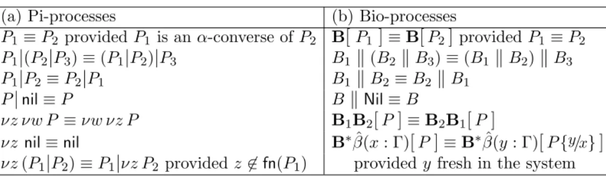
Table 1: Laws for structural congruence.
(a) Pi-processes (b) Bio-processes
P1 ≡ P2 provided P1 is an α-converse of P2 B[P1 ]≡ B[P2]provided P1 ≡ P2
P1|(P2|P3) ≡ (P1|P2)|P3 B1 "(B2 "B3) ≡ (B1"B2)"B3
P1|P2≡ P2|P1 B1 "B2≡ B2"B1
P|nil≡ P B"Nil≡ B
νz νw P ≡ νw νz P B1B2[P]≡ B2B1[P]
νz nil≡ nil B∗β(x : Γ)ˆ [P]≡ B∗β(y : Γ)ˆ [P{y/x}]
νz (P1|P2) ≡ P1|νz P2 provided z (∈ fn(P1) provided y fresh in the system
Definition 2 The reduction relation −→ is the smallest relation over
bio-processes obtained by applying the axioms and rules in Table 2.
4
Causality, Enabling and Concurrency
We first introduce two auxiliary functions, l and subj, to simplify the pre-sentation of our subsequent treatment. For each action µ and ρ, the function
l specifies its type, while the function subj specifies the name it operates
on (i.e. for input/output actions it is the name of the channel on which it receives/sends, while for expose/hide/unhide actions it is the subject of the beta binder).
l(x(w)) = in l("x(w)!) = in inter l(xw) = out l("xw!) = out inter l(expose(x, ∆)) = expose l(join P ) = join l(hide(x)) = hide l(split&P0, P1') = split
l(unhide(x)) = unhide
subj(x(w)) = subj(xw) = subj("x(w)!) = subj("xw!) = {x} subj(expose(x, ∆)) = subj(hide(x)) = subj(unhide(x)) ={x} subj(join P ) = subj(split&P0, P1') = ⊥
Hereafter, we assume that all the bound names in the system are not used except for their bound occurrences. In general it is possible to modify any system to satisfy this constraint by applying α-conversion. We also
Table 2: Axioms and rules for the reduction relation. (intra) P ≡ ν ˜u (ϕϕ0x(w). P0|ϕϕ1xz. P1|P2) ϑB[P ]ϑϕ$ϕ0x(w)−→,ϕ1xz%ϑB[ν ˜u (ϕϕ0P0{z/w}|ϕϕ1P1|P2)] (inter) P ≡ ν ˜u (ϕ0x(w). P1|P2) Q≡ ν˜v (ϕ1yz. Q1|Q2)
X ϑ$&iϑ0ϕ0!x(w)−→!,&1−iϑ1ϕ1!yz! Y
where X = ϑ"iϑ0β(x : Γ) B∗0[P ]"ϑ"1−iϑ1β(y : ∆) B∗1[Q],
Y = ϑ"iϑ0β(x : Γ) B∗0[P" ]"ϑ"1−iϑ1β(y : ∆) B∗1[Q" ],
P"= ν ˜u (ϕ0P1{z/w}|P2) and Q"= ν˜v (ϕ1Q1|Q2)
provided Γ ∩ ∆ (= ∅ and x, z /∈ ˜u and y, z /∈ ˜v (expose)
P ≡ ν ˜u (ϕ expose(x, Γ) . P1|P2)
ϑB[P ]ϑϕ expose(x, Γ)−→ ϑB β(y : Γ)[ν ˜u (ϕP1{y/x}|P2)]
provided y fresh in the system (hide) P ≡ ν ˜u (ϕ hide(x) . P1|P2) ϑB∗β(x : Γ)[P ]ϑϕ hide(x)−→ ϑB∗βh(x : Γ)[ν ˜u (ϕP1|P2)] provided x /∈ ˜u (unhide) P ≡ ν ˜u (ϕ unhide(x) . P1|P2) ϑB∗βh(x : Γ)[P ]ϑϕ unhide(x)−→ ϑB∗β(x : Γ)[ν ˜u (ϕP1|P2)] provided x /∈ ˜u (join) ϑ"0ϑ0B0[P0 ]"ϑ"1ϑ1B1[P1 ]
ϑ$&0ϑ0join P0,&1ϑ1join P1%
−→ Y
where Y = ϑ"0ϑ0B[|0P0σ0||1P1σ1 ]"ϑ"1ϑ1Nil
provided that fjoin is defined in (B0, B1, P0, P1)
and with fjoin(B0, B1, P0, P1) = (B, σ0, σ1)
(split) ϑB[P0|P1 ]
ϑ split$P0,P1%
−→ ϑ"0B0[P0σ0 ]"ϑ"1B1[P1σ1 ]
provided that fsplit is defined in (B, P0, P1)
and with fsplit(B, P0, P1) = (B0, B1, σ0, σ1)
(bang) ϑB[P|Q] θ −→ ϑB"[P"|Q" ] ϑB[!P|Q]−→ ϑB!θ "[!P|P"|Q" ] (redex) B θ −→ B" B "B"" −→ Bθ ""B"" (struct) B1 ≡ B " 1 B"1 θ −→ B2 B1−→ Bθ 2
assume that all the names in the system are marked by an index and that at the beginning of the computation its value is 0. Moreover, the new name introduced by the expose operation is the same as the bound name in the primitive with the index incremented by one (e.g. B[ expose(xn, ∆) .P ]−→
B β(xn+1 : ∆)[P{xn+1/xn} ]).
4.1 Causal Relation
Now we can define the causal relation between pairs of transitions in a computation. Recall that an activity A causes an activity B if A influences the execution of B. Our labels allow us to use them as unique names for the transitions as they are linearizations encoding the position of the prefixes and processes originating the transitions in the syntax tree.
Definition 3 (Immediate causal relation) Given a computation B0−→θ0
B1 −→ · · ·θ1 −→ Bθn n+1, we say that θn immediately depends on θh (or,
sym-metrically, θh immediately causes θn) if h < n and θh! θn can be derived
by repeated applications of the following rules, where i, j ∈ {0, 1}. 1. "iθ! "iθ" if θ ! θ" 2. |iδ! |iδ" if δ ! δ" 3. !δ ! |0δ" 4. !δ ! |1δ" if δ ! δ" 5. θ ! &θ" 0, θ"1' if ∃i.θ ! θ"i 6. &θ0, θ1' ! θ" if ∃i.θi! θ"
7. &θ0, θ1' ! &θ"0, θ"1' if ∃i, j.θi! θ"j
8. µ ! ϕµ" if (l(µ) = in ∨ l(µ) = in inter ∨ l(µ) = expose)
9.
ϕµ! ϕ"µ" if (subj(µ) = subj(µ") ∧
((l(µ)=hide ∧ l(µ")=unhide) ∨
(l(µ)=unhide ∧ l(µ")=hide) ∨
(l(µ)=unhide ∧ (l(µ")=in inter ∨ l(µ")=out inter))))
10. ϕµ ! ρ 11. ρ ! ϕµ 12. ρ ! ϑρ
The rules listed above are applied recursively to a pair of actions θh, θn
in order to verify if there is a structural dependency between them.
The recursive step is implemented by removing the common prefixes of
θh and θnthrough rules 1 and 2. First, rule 1 is applied since it concerns the
labels of the bio-processes; then, if θh and θn refer to the same bio-process,
while for Beta-binders two levels of recursion are needed to take into account the parallel structure of both bio-processes and pi-processes.
Rules 3 and 4 take into account the replication operator and are analo-gous to the ones for the π-calculus, as described in [4].
Rules 5, 6 and 7 state that a coupled action (a communication or a join) is caused by/causes another action if one of the two partners of the coupled action is caused by/causes the other action.
Rules 8, 9, 10, 11 and 12 are applied at the end of the recursive steps and are peculiar to Beta-binders, since they are relative to the operators which are peculiar in Beta-binders.
Rule 8 describes the causal dependency imposed by the sequential struc-ture of the pi-processes: an action θh = ϑϕµ causes an action θnwhose label
has ϑϕ as a prefix if θh is a binder (i.e. if θh is an input action (either in an
internal or in an inter-communication) or an expose operation). The idea which lead to the definition of this rule is that all binder operators cause a flow of information to their suffix, so they must cause them. The third case, the expose operator, is peculiar to Beta-binders: since it introduces a new beta binder on the interface of the process, the rest of the process is considered to be necessarily caused by it.
Rule 9 describes how the operations on the interfaces influence each other: an hide causes an unhide of the same beta binder; an unhide causes an hide of the same beta binder or an inter-communication on it; this causal dependency holds both if the address label of θh is a prefix of the one of θn
and if they just refer to the same bio-process.
Rules 10, 11 and 12 are relative to the causal relation between actions happening within a process and join/split functions involving that bio-process.
Rule 10 states that an operation that involves one of the bio-processes later merged by a join or divided by a split causes the execution of that function; for example the introduction of a new binder in the interface of a bio-process can be fundamental for the subsequent application of fjoin and
fsplit functions.
Rule 11 and 12 state that join and split operations cause all the opera-tions that involve the bio-processes obtained after their execution (commu-nications, operations on the interfaces, join and split operations).
The definition of the causal relation between two transitions of a com-putation is obtained by taking into account the transitive closure of the immediate causal relation.
Definition 4 (Causal relation) Let < ! (!)∗ be the transitive closure of
!. Then, given a computation B0−→ Bθ0 1−→ · · ·θ1 −→ Bθn n+1, we say that θn
depends on θh (or, symmetrically, θh causes θn) if θh < θn.
4.2 Enabling Relation
In this section we define the enabling relation between pairs of transitions in a computation. Recall that an activity A enables an activity B if either
A is a necessary condition for the execution of B or A cannot be executed after B.
Definition 5 (Immediate enabling relation) Given a computation B0 −→θ0
B1−→ · · ·θ1 −→ Bθn n+1, we say that θn is immediately enabled by θh (or,
sym-metrically, θh immediately enables θn) if h < n and θh/· θn can be derived
by repeated applications of the following rules, where i, j ∈ {0, 1}. 1. "iθ/· "iθ" if θ /· θ" 2. |iδ/· |iδ" if δ /· δ" 3. !δ /· |0δ" 4. !δ /· |1δ" if δ /· δ" 5. θ /· &θ" 0, θ1"' if ∃i.θ /· θ"i 6. &θ0, θ1' /· θ" if ∃i.θi/· θ"
7. &θ0, θ1' /· &θ"0, θ"1' if ∃i, j.θi /· θ"j
8. µ /· ϕµ"
9. ϕi /· ϕ"b if (l(b) = hide∧ subj(i) = subj(b))
10. ϕµ /· ρ
Rules 1-7 are analogous to rules 1-7 in Def. 3 for causality.
Rule 8 describes the temporal dependency imposed by the sequential structure of the pi-processes: every action θh = ϑϕµ causes an action θn
whose label has ϑϕ as a prefix. This rule is a generalization of the respective one for causality, without the constraint on the type of the action µ.
Rules 9 and 10 are peculiar to Beta-binders.
Rule 9 describes the temporal dependency between an inter-communication and an hide operation on the same beta binder: in fact it is not possible to execute the inter-communication after the beta binder is hidden.
Rule 10 is analogous to rule 10 in Def. 3 for causality.
The definition of the enabling relation between two transitions of a com-putation is obtained by taking into account the transitive closure of the immediate enabling relation.
Definition 6 (Enabling relation) Let / ! (/·)∗be the transitive closure
of /·. Then, given a computation B0 −→ Bθ0 1 −→ · · ·θ1 −→ Bθn n+1, we say that
θn is enabled by θh (or, symmetrically, θh enables θn) if θh/ θn.
We decided to keep the relation of causality and that of enabling distinct because they are logically different and, moreover, to be consistent with the analogous definitions for π-calculus proposed in the literature. In the following part, however, we will merge them in a single relation (their union) and we will only consider the latter.
The following propositions show that causality and enabling are distinct relations.
Proposition 1 < " /.
Proof. Consider θ0 = ϑϕ hide(x) and θ1 = ϑϕ"unhide(x). It is θ0 < θ1 but
θ0 (/ θ1.
Proposition 2 / " <.
Proof. Consider θ0 = ϑϕ hide(x) and θ1 = ϑϕ"&ϕ0y(w), ϕ1yz', where ϕ =
ϕ"ϕ0. It is θ0/ θ1 but θ0 ≮ θ1.
4.3 Concurrency Relation
Recall that two activities A and B are concurrent if they can be executed in parallel.
Definition 7 (Concurrency relation) Let ≺ ! (< ∪ /)∗. Then, given
a system B, we say that θn and θh are concurrent (i.e. they can be
exe-cuted simultaneously, written θn+ θh) if ∀ computation ξ = B −→∗ B" s.t.
θn, θh ∈ ξ . θn⊀ θh and θh⊀ θn.
5
Properties of the Concurrency Relation
In this sections we state two lemmas and two corollaries and one theorem derived from them.
The first lemma states that if two consecutive transitions in a compu-tation are concurrent, then they form a diamond in the proved transition system.
Lemma 1 Given a computation B0 −→ Bθ0 1 −→ Bθ1 2, if θ0⊀ θ1 ⇒ ∃B1".B0−→θ1
B"
1
θ0
−→ B2. In other words, the following diagram exists:
B0
θ04 5θ1
B1 B1"
θ15 4θ0
B2
Proof. We have by hypothesis that B0 −→ Bθ0 1 −→ Bθ1 2 and θ0 ⊀ θ1 (in
particular, since θ0 and θ1are consecutive transactions, we have that θ0(! θ1
and θ0 (/· θ1).
The proof is done by cases on the labels of the transitions. 1. θ0 = ϑϕ expose(x, ∆):
(a) θ1 = ϑ"ϕ"expose(y, Γ): by Def. 3, θ0! θ1 iff ϑϕ is a prefix of ϑ"ϕ"
(rule 8); by Def. 5, θ0 /· θ1 iff ϑϕ is a prefix of ϑ"ϕ" (rule 8); by
hypothesis θ0 (! θ1 and θ0 (/· θ1, hence ϑϕ is not a prefix of ϑ"ϕ";
if ϑ (= ϑ", then θ0 and θ1 refer to different bio-processes, so it
is possible to exchange their order without any consequence; if, otherwise, ϑ = ϑ" and ϕ is not a prefix of ϕ", then θ
0 and θ1 refer
to the same bio-process but to different pi-processes, so they can be exchanged as well (recall that we have assumed that x (= y, so the two expose operations do not influence each other);
(b) θ1 = ϑ"ϕ"hide(y): by Def. 3, θ0 ! θ1 iff ϑϕ is a prefix of ϑ"ϕ"
(rule 8); by Def. 5, θ0 /· θ1 iff ϑϕ is a prefix of ϑ"ϕ" (rule 8);
hence ϑϕ is not a prefix of ϑ"ϕ", so θ
0 and θ1 refer to different
beta binders (recall that x is only available for actions with the same prefix as θ0, so x (= y); so they can be exchanged;
(c) θ1 = ϑ"ϕ"unhide(y): by Def. 3, θ0! θ1 iff ϑϕ is a prefix of ϑ"ϕ"
(rule 8); by Def. 5, θ0 /· θ1 iff ϑϕ is a prefix of ϑ"ϕ" (rule 8);
hence ϑϕ is not a prefix of ϑ"ϕ", so θ
0 and θ1 refer to different
beta binders (again, x is only available for actions with the same prefix as θ0, so x (= y); so they can be exchanged;
(d) θ1 = ϑ"ϕ"&ϕ0y(t), ϕ1yz': by Def. 3, θ0! θ1 iff ϑϕ is a prefix of
ϑ"ϕ"ϕ0 or of ϑ"ϕ"ϕ1 (rule 8); by Def. 5, θ0 /· θ1 iff ϑϕ is a prefix
of ϑ"ϕ"ϕ
0 or of ϑ"ϕ"ϕ1 (rule 8); hence ϑϕ is a prefix of none of
them, so θ0 and θ1 can be exchanged since expose operations and
internal communications do not influence each other;
(e) θ1 = ϑ"&"iϑ0ϕ0y(t),"1−iϑ1ϕ1wz': by Def. 3, θ0 ! θ1 iff ϑϕ is a
prefix of ϑ""
iϑ0ϕ0 or of ϑ""1−iϑ1ϕ1 (rule 8); by Def. 5, θ0 /· θ1
iff ϑϕ is a prefix of ϑ""iϑ0ϕ0 or of ϑ""1
−iϑ1ϕ1 (rule 8); hence ϑϕ
is a prefix of none of them, so θ0 and θ1 do not influence each
other since they refer to different beta binders (again, x is only available for actions with the same prefix as θ0, so x (= y and
x(= w); so they can be exchanged;
(f) θ1 = ϑ"&"0ϑ0join Q0,"1ϑ1join Q1': by Def. 3, θ0!θ1 iff ϑ = ϑ""0ϑ0
or ϑ = ϑ""1ϑ1 (rule 10); by Def. 5, θ0 /· θ1 iff ϑ = ϑ""0ϑ0
or ϑ = ϑ""
1ϑ1 (rule 10); hence θ0 and θ1 refer to different
bio-processes, so they can be exchanged;
(g) θ1 = ϑ"split&Q0, Q1': by Def. 3, θ0! θ1 iff ϑ = ϑ" (rule 10); by
Def. 5, θ0 /· θ1 iff ϑ = ϑ" (rule 10); hence θ0 and θ1 refer to
different bio-processes, so they can be exchanged; 2. θ0 = ϑϕ hide(x):
(a) θ1 = ϑ"ϕ"expose(y, ∆): by Def. 5, θ0 /· θ1 iff ϑϕ is a prefix of
ϑ"ϕ" (rule 8); hence ϑϕ is not a prefix of ϑ"ϕ", so θ0 and θ1 refer to
different beta binders (again, y is only available for actions with the same prefix as θ1, so x (= y); so they can be exchanged;
(b) θ1 = ϑ"ϕ"hide(y): by Def. 5, θ0 /· θ1 iff ϑϕ is a prefix of ϑ"ϕ"
it is not possible to execute two hide operations on the same beta binder consecutively), so they can be exchanged;
(c) θ1 = ϑ"ϕ"unhide(y): by Def. 3, θ0!θ1iff ϑ = ϑ"and x = y (rule 9);
by Def. 5, θ0 /· θ1 iff ϑϕ is a prefix of ϑ"ϕ" (rule 8); hence ϑϕ is
not a prefix of ϑ"ϕ" and x (= y, so they can be exchanged, since
the two operations do not influence each other;
(d) θ1 = ϑ"ϕ"&ϕ"0y(t), ϕ"1yu': by Def. 5, θ0 /· θ1 iff ϑϕ is a prefix of
ϑ"ϕ"ϕ"0 or of ϑ"ϕ"ϕ"1 (rule 8); hence ϑϕ is a prefix of none of them,
so θ0 and θ1 can be exchanged since hide operations and internal
communications do not influence each other;
(e) θ1 = ϑ"&"iϑ0ϕ"0y(t),"1−iϑ1ϕ"1vu': by Def. 5, θ0 /· θ1 iff ϑϕ is
a prefix of ϑ""iϑ0ϕ"
0 or of ϑ""1−iϑ1ϕ"1 (rule 8); hence ϑϕ is a
prefix of none of them; moreover, x (= y and x (= v (since it is not possible to execute an inter-communication immediately after an hide operation on the same beta binder), so they can be exchanged;
(f) θ1 = ϑ"&"0ϑ0join Q0,"1ϑ1join Q1': by Def. 3, θ0!θ1 iff ϑ = ϑ""0ϑ0
or ϑ = ϑ""
1ϑ1 (rule 10); by Def. 5, θ0 /· θ1 iff ϑ = ϑ""0ϑ0
or ϑ = ϑ""
1ϑ1 (rule 10); hence θ0 and θ1 refer to different
bio-processes, so they can be exchanged;
(g) θ1 = ϑ"split&Q0, Q1': by Def. 3, θ0! θ1 iff ϑ = ϑ" (rule 10); by
Def. 5, θ0 /· θ1 iff ϑ = ϑ" (rule 10); hence θ0 and θ1 refer to
different bio-processes, so they can be exchanged; 3. θ0 = ϑϕ unhide(x):
(a) θ1 = ϑ"ϕ"expose(y, ∆): by Def. 5, θ0 /· θ1 iff ϑϕ is a prefix of
ϑ"ϕ" (rule 8); hence ϑϕ is not a prefix of ϑ"ϕ", so θ0 and θ1 refer to
different beta binders (again, y is only available for actions with the same prefix as θ1, so x (= y); so they can be exchanged;
(b) θ1 = ϑ"ϕ"hide(y): by Def. 3, θ0! θ1 iff ϑ = ϑ" and x = y (rule 9);
by Def. 5, θ0 /· θ1 iff ϑϕ is a prefix of ϑ"ϕ" (rule 8); hence ϑϕ is
not a prefix of ϑ"ϕ" and x (= y, so they can be exchanged, since
the two operations do not influence each other;
(c) θ1 = ϑ"ϕ"unhide(y): by Def. 5, θ0 /· θ1 iff ϑϕ is a prefix of ϑ"ϕ"
(rule 8); hence ϑϕ is not a prefix of ϑ"ϕ"; moreover, x (= y (since
it is not possible to execute two unhide operations on the same beta binder consecutively), so they can be exchanged;
(d) θ1 = ϑ"ϕ"&ϕ"0y(t), ϕ"1yu': by Def. 5, θ0 /· θ1 iff ϑϕ is a prefix
of ϑ"ϕ"ϕ"
0 or of ϑ"ϕ"ϕ"1 (rule 8); hence ϑϕ is a prefix of none of
them, so θ0 and θ1 can be exchanged since unhide operations and
internal communications do not influence each other;
(e) θ1 = ϑ"&"iϑ0ϕ"0y(t),"1−iϑ1ϕ"1vu': by Def. 3, θ0!θ1iff (ϑ = ϑ""iϑ0
and x = y) or (ϑ = ϑ""
1−iϑ1 and x (= v) (rule 9); by Def. 5,
θ0 /· θ1 iff ϑϕ is a prefix of ϑ""iϑ0ϕ0" or of ϑ""1−iϑ1ϕ"1 (rule 8);
hence ϑϕ is a prefix of none of them and θ0and θ1refer to different
(f) θ1 = ϑ"&"0ϑ0join Q0,"1ϑ1join Q1': by Def. 3, θ0!θ1 iff ϑ = ϑ""0ϑ0
or ϑ = ϑ""
1ϑ1 (rule 10); by Def. 5, θ0 /· θ1 iff ϑ = ϑ""0ϑ0
or ϑ = ϑ""
1ϑ1 (rule 10); hence θ0 and θ1 refer to different
bio-processes, so they can be exchanged;
(g) θ1 = ϑ"split&Q0, Q1': by Def. 3, θ0! θ1 iff ϑ = ϑ" (rule 10); by
Def. 5, θ0 /· θ1 iff ϑ = ϑ" (rule 10); hence θ0 and θ1 refer to
different bio-processes, so they can be exchanged; 4. θ0 = ϑϕ&ϕ0x(w), ϕ1xz':
(a) θ1 = ϑ"ϕ"expose(y, ∆): by Def. 3, θ0! θ1 iff ϑϕϕ0 is a prefix of
ϑ"ϕ"(rule 8); by Def. 5, θ0/· θ1iff either ϑϕϕ0 or ϑϕϕ1is a prefix
of ϑ"ϕ" (rule 8); hence θ0 and θ1 can be exchanged, since the two
operations do not influence each other;
(b) θ1 = ϑ"ϕ"hide(y): by Def. 3, θ0 ! θ1 iff ϑϕϕ0 is a prefix of ϑ"ϕ"
(rule 8); by Def. 5, θ0 /· θ1 iff either ϑϕϕ0 or ϑϕϕ1 is a prefix of
ϑ"ϕ" (rule 8); hence θ0 and θ1 can be exchanged;
(c) θ1 = ϑ"ϕ"unhide(y): by Def. 3, θ0! θ1 iff ϑϕϕ0 is a prefix of ϑ"ϕ"
(rule 8); by Def. 5, θ0 /· θ1 iff either ϑϕϕ0 or ϑϕϕ1 is a prefix of
ϑ"ϕ" (rule 8); hence θ0 and θ1 can be exchanged;
(d) θ1 = ϑ"ϕ"&ϕ"0y(t), ϕ"1yu': by Def. 3, θ0! θ1 iff ϑϕϕ0 is a prefix of
ϑ"ϕ"ϕ"
0 or of ϑ"ϕ"ϕ"1 (rule 8); by Def. 5, θ0 /· θ1 iff either ϑϕϕ0 or
ϑϕϕ1 is a prefix of ϑ"ϕ"ϕ"0 or of ϑ"ϕ"ϕ"1 (rule 8); hence θ0 and θ1
can be exchanged;
(e) θ1 = ϑ"&"iϑ0ϕ"0y(t),"1−iϑ1ϕ"1vu': by Def. 3, θ0! θ1 iff ϑϕϕ0 is a
prefix of ϑ""
iϑ0ϕ"0 or of ϑ""1−iϑ1ϕ"1 (rule 8); by Def. 5, θ0 /· θ1
iff either ϑϕϕ0 or ϑϕϕ1 is a prefix of ϑ""iϑ0ϕ"0 or of ϑ""1−iϑ1ϕ"1
(rule 8); hence θ0 and θ1 can be exchanged;
(f) θ1 = ϑ"&"0ϑ0join Q0,"1ϑ1join Q1': by Def. 3, θ0!θ1 iff ϑ = ϑ""0ϑ0
or ϑ = ϑ""
1ϑ1 (rule 10); by Def. 5, θ0 /· θ1 iff ϑ = ϑ""0ϑ0
or ϑ = ϑ""
1ϑ1 (rule 10); hence θ0 and θ1 refer to different
bio-processes, so they can be exchanged;
(g) θ1 = ϑ"split&Q0, Q1': by Def. 3, θ0! θ1 iff ϑ = ϑ" (rule 10); by
Def. 5, θ0 /· θ1 iff ϑ = ϑ" (rule 10); hence θ0 and θ1 refer to
different bio-processes, so they can be exchanged; 5. θ0 = ϑ&"iϑ0ϕ0x(w),"1−iϑ1ϕ1yz':
(a) θ1 = ϑ"ϕ"expose(t, ∆): by Def. 3, θ0! θ1 iff ϑ"iϑ0ϕ0 is a prefix of
ϑ"ϕ" (rule 8); by Def. 5, θ0 /· θ1 iff either ϑ"iϑ0ϕ0 or ϑ"1−iϑ1ϕ1
is a prefix of ϑ"ϕ" (rule 8); hence θ
0 and θ1 can be exchanged;
(b) θ1 = ϑ"ϕ"hide(t): by Def. 3, θ0! θ1 iff ϑ"iϑ0ϕ0 is a prefix of ϑ"ϕ"
(rule 8); by Def. 5, θ0 /· θ1 iff (either ϑ"iϑ0ϕ0 or ϑ"1−iϑ1ϕ1 is a
prefix of ϑ"ϕ") (rule 8) or (ϑ"
iϑ0 = ϑ"and x = t) or (ϑ"1−iϑ1= ϑ"
and y = t) (rule 9); hence θ0 and θ1 refer to pi-processes and
(c) θ1 = ϑ"ϕ"unhide(t): by Def. 3, θ0 ! θ1 iff ϑ"iϑ0ϕ0 is a prefix of
ϑ"ϕ" (rule 8); by Def. 5, θ0 /· θ1 iff either ϑ"iϑ0ϕ0 or ϑ"1−iϑ1ϕ1
is a prefix of ϑ"ϕ" (rule 8); moreover, θ
0 and θ1 refer to
differ-ent binders (since it is not possible to execute an unhide opera-tion immediately after an inter-communicaopera-tion on the same beta binder), so they can be exchanged;
(d) θ1 = ϑ"ϕ&ϕ"0v(t), ϕ"1vu': by Def. 3, θ0! θ1 iff ϑ"iϑ0ϕ0 is a prefix
of ϑ"ϕϕ"
0 or of ϑ"ϕϕ"1 (rule 8); by Def. 5, θ0 /· θ1iff either ϑ"iϑ0ϕ0
or ϑ"1−iϑ1ϕ1 is a prefix of ϑ"ϕϕ"0 or of ϑ"ϕϕ"1 (rule 8); hence θ0
and θ1 can be exchanged;
(e) θ1 = ϑ"&"iϑ"0ϕ"0v(t),"1−iϑ"1ϕ"1ru': by Def. 3, θ0! θ1 iff ϑ"iϑ0ϕ0
is a prefix of ϑ""
iϑ"0ϕ"0 or of ϑ""1−iϑ"1ϕ"1 (rule 8); by Def. 5, θ0 /
· θ1 iff either ϑ"iϑ0ϕ0 or ϑ"1−iϑ1ϕ1 is a prefix of ϑ""iϑ"0ϕ"0 or of
ϑ""1−iϑ"1ϕ"1 (rule 8); hence θ0 and θ1 can be exchanged;
(f) θ1 = ϑ"&"0ϑ"0join Q0,"1ϑ"1join Q1': by Def. 3, θ0 ! θ1 iff ϑ"iϑ0
or ϑ"1ϑ1 are equal to ϑ""0ϑ"0 or to ϑ""1ϑ"1 (rule 10); by Def. 5,
θ0 /· θ1 iff ϑ"iϑ0 or ϑ"1ϑ1 are equal to ϑ""0ϑ"0 or to ϑ""1ϑ"1
(rule 10); hence θ0 and θ1 refer to different bio-processes, so they
can be exchanged;
(g) θ1 = ϑ"split&Q0, Q1': by Def. 3, θ0!θ1iff ϑ"iϑ0 = ϑ" or ϑ"1−iϑ1 =
ϑ" (rule 10); by Def. 5, θ0 /· θ1 iff ϑ"iϑ0 = ϑ" or ϑ"1−iϑ1 = ϑ"
(rule 10); hence θ0 and θ1 refer to different bio-processes, so they
can be exchanged;
6. θ0 = ϑ &"0ϑ0join Q0,"1ϑ1join Q1':
(a) θ1 = ϑ"ϕ expose(x, ∆): by Def. 3, θ0! θ1 iff ϑ"0ϑ0= ϑ" (rule 11);
hence θ0 and θ1 refer to different bio-processes and so they can
be exchanged;
(b) θ1 = ϑ"ϕ hide(x): by Def. 3, θ0 ! θ1 iff ϑ"0ϑ0 = ϑ" (rule 11);
hence θ0 and θ1 refer to different bio-processes and so they can
be exchanged;
(c) θ1 = ϑ"ϕ unhide(x): by Def. 3, θ0! θ1 iff ϑ"0ϑ0 = ϑ" (rule 11);
hence θ0 and θ1 refer to different bio-processes and so they can
be exchanged;
(d) θ1 = ϑ"ϕ&ϕ0y(w), ϕ1yz': by Def. 3, θ0!θ1iff ϑ"0ϑ0= ϑ" (rule 11);
hence θ0 and θ1 refer to different bio-processes and so they can
be exchanged;
(e) θ1 = ϑ"&"iϑ"0ϕ0y(t),"1−iϑ"1ϕ1wz': by Def. 3, θ0! θ1 iff ϑ"0ϑ0 =
ϑ""iϑ"0 or ϑ"0ϑ0 = ϑ""1−iϑ"1 (rule 11); hence θ0 and θ1 refer to
different bio-processes and so they can be exchanged;
(f) θ1 = ϑ"&"0ϑ"0join Q"0,"1ϑ"1join Q"1': by Def. 3, θ0! θ1 iff ϑ"0ϑ0 =
ϑ""iϑ"0 or ϑ"0ϑ0 = ϑ""1−iϑ"1 (rule 12); hence θ0 and θ1 refer to
different bio-processes and so they can be exchanged;
(g) θ1 = ϑ"split&Q"0, Q"1': by Def. 3, θ0! θ1 iff ϑ"0ϑ0 = ϑ" (rule 12);
hence θ0 and θ1 refer to different bio-processes and so they can
7. θ0 = ϑ split&Q0, Q1':
(a) θ1 = ϑ"ϕ expose(x, ∆): by Def. 3, θ0! θ1 iff ϑ"j = ϑ" (rule 11);
hence θ0 and θ1 refer to different bio-processes and so they can
be exchanged;
(b) θ1 = ϑ"ϕ hide(x): by Def. 3, θ0! θ1 iff ϑ"j = ϑ" (rule 11); hence
θ0 and θ1 refer to different bio-processes and so they can be
ex-changed;
(c) θ1 = ϑ"ϕ unhide(x): by Def. 3, θ0 ! θ1 iff ϑ"j = ϑ" (rule 11);
hence θ0 and θ1 refer to different bio-processes and so they can
be exchanged;
(d) θ1 = ϑ"ϕ&ϕ0y(w), ϕ1yz': by Def. 3, θ0! θ1 iff ϑ"j = ϑ" (rule 11);
hence θ0 and θ1 refer to different bio-processes and so they can
be exchanged;
(e) θ1 = ϑ"&"iϑ0ϕ0y(t),"1−iϑ1ϕ1wz': by Def. 3, θ0 ! θ1 iff ϑ"j =
ϑ""iϑ0 or ϑ"j = ϑ""1−iϑ1 (rule 11); hence θ0 and θ1 refer to
dif-ferent bio-processes and so they can be exchanged;
(f) θ1 = ϑ"&"0ϑ"0join Q"0,"1ϑ"1join Q"1': by Def. 3, θ0 ! θ1 iff ϑ"j =
ϑ""0ϑ"0or ϑ"j = ϑ""1ϑ"1(rule 12); hence θ0and θ1refer to different
bio-processes and so they can be exchanged;
(g) θ1 = ϑ"split&Q"0, Q1"': by Def. 3, θ0 ! θ1 iff ϑ"j = ϑ" (rule 12);
hence θ0 and θ1 refer to different bio-processes and so they can
be exchanged.
Corollary 1 Given a computation B0 −→ Bθ0 1 −→ Bθ1 2, if θ0 + θ1 ⇒
∃B"
1.B0 −→ Bθ1 1"
θ0
−→ B2.
The second lemma, usually known as permutation of transitions, states that there always exists a computation in which two concurrent transitions occur consecutively.
Lemma 2 Given a computation ξ = B0 −→ Bθ0 1 −→ · · · −→ Bn −→ Bθn n+1,
if θ0 ⊀ θn ⇒ ∃ a permutation σ : [0..n] → [0..n] and a computation B0
θ! 0 −→ B1" θ!1 −→ · · · Bn" θ!n
−→ Bn+1 such that ∃i ∈ [0..n] .(σ(0) = i ∧ σ(n) = i + 1 ∧
σ(j) = j− 1 for 0 < j ≤ i ∧ σ(m) = m + 1 for i + 1 ≤ m < n) with θ"
σ(l) = θl
for each l ∈ [0..n].
Proof. The proof is by induction on the length n of the computation. • Induction basis
n = 1 (i.e. ξ = B0 −→ Bθ0 1 −→ Bθ1 2 and θ0 ⊀ θ1 (hence θ0 (! θ1 and
θ0 (/· θ1)).
The permutation is σ : [0, 1] → [0, 1] and the computation ξ satisfies the properties.
• Inductive step
Let us assume that the lemma holds for n = k (i.e. k − 1 transitions between θ0 and θn); now let us consider n = k + 1 (i.e. k transitions
between θ0 and θn).
Let h be the minimum index such that θ0 ⊀ θh; hence θl ⊀ θhholds for
any l < h (because if per absurdum θl ≺ θh (i.e. θl ≮ θh or θl (/ θh),
then, for the transitive property of < and /, θ0 ≺ θh). Hence, by
Lemma 1 we can swap θh and θh−1in ξ, obtaining ξ1= B0−→ · · · −→θ0
Bh−1 θh
−→ Bh" θh−1
−→ Bh+1 −→ · · · −→ Bθn n+1. We can then repeat this
procedure h times, until we obtain ξh = B
0 −→ Bθh "0
θ0
−→ · · ·−→ Bθn n+1,
in which there are k − 1 transitions between θ0 and θn, so that it is
possible to apply the inductive hypothesis.
Corollary 2 Given a computation ξ = B0 −→ Bθ0 1 −→ · · · −→ Bn −→θn
Bn+1, if θ0 + θn⇒ ∃ a permutation σ : [0..n] → [0..n] and a computation B0
θ! 0 −→ B1" θ!1 −→ · · · Bn" θ!n
−→ Bn+1 such that ∃i ∈ [0..n] .(σ(0) = i ∧ σ(n) = i + 1 ∧
σ(j) = j− 1 for 0 < j ≤ i ∧ σ(m) = m + 1 for i + 1 ≤ m < n) with θ"σ(l) = θl
for each l ∈ [0..n].
The following theorem derives from Corollary 1 and Corollary 2 and it states that if in a computation there are two concurrent transitions, then there exists another computation in which the two transitions occur in re-verse order.
Theorem 1 Given a computation B0 −→ · · ·θ0 −→ Bθn n+1, if θ0 + θn ⇒ ∃ a
computation B0 −→ · · ·−→ · · ·θn −→ · · · −→ Bθ0 n+1.
6
Application to Biology, Pharmacology and Medicine
There are many potential applications of this technology. One interesting application is in biology: by analysing these properties, life scientists could obtain interesting predictions on the dynamical behaviour of complex sys-tems under investigation (for example the interaction of distinct entities in signalling pathways).
Another application is in pharmacology: causality and concurrency anal-ysis of a system made up of an ill organism and a new drug to be tested can assist pharmacologists by identifying the effects (both positive and negative) of the new drug on the organism. Compared to the traditional method used in drug discovery, which is to test a new drug on animals and then on a small number of selected human beings, the method provided by software is faster and safer, so that “in vivo” tests can be done at a lower risk. Hence, computer simulation with causality and concurrency analysis can greatly help pharmacologists, who need to specify the system composed of the ill organism and the drug, to select a set of relevant tests to be performed on animals and human beings.
Finally, another application is in medicine: causality analysis can assist doctors in medical diagnosis by allowing them to consider only the events and the subpart of the organism which are relevant to the abnormal behaviour under investigation; this is very important in medicine since the organism under investigation, the human body, is a huge and complex system, which is definitely intractable altogether.
6.1 An Example: the ERK/MAPK Pathway
In this section we model and analyse the ERK pathway, which is an instance of the important and intensively studied MAPK pathway. The term ‘MAPK pathway’ refers to a module of three kinases activated by sequentially phos-phorylating each other.
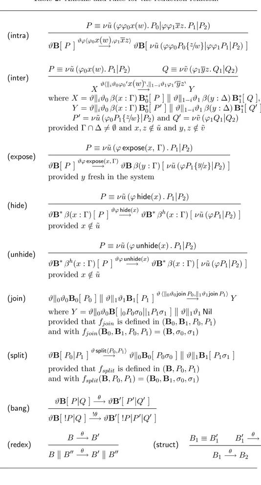
Figure 1 shows the Raf/MEK/ERK pathway (see [8] for details).
Figure 1: Structure of the ERK pathway.
The binding of a ligand to RTK (receptor tyrosine kinase) causes the autophosphorylation of RTK on tyrosine residues, which are docking sites for adaptor and signalling molecules.
By means of the adaptor proteins Shc and Grb, Ras recruits SOS (a GDP/GTP exchange factor), which allows Ras to be activated; symmetri-cally, by means of the adaptor protein Crk, Rap1 recruits C3G (a GDP/GTP exchange factor), which allows Rap1 to be activated.
Ras can activate two types of Raf proteins (Raf-1 and B-Raf), while Rap1 can only activate B-Raf.
Both types of Raf proteins can activate MEK-1/2 by phosphorylation on two serine residues.
MEK-1/2 can activate ERK-1/2 by phosphorylation on threonine and tyrosine residues.
Upon activation, ERK can phosphorylate over 80 substrates in the cy-toplasm and the nucleus, and it can regulate gene expression by phosphory-lating transcription factors such Ets, Elk and Myc.
Negative feedback loops include the induction of MKPs by ERK, and the inhibitory phosphorylation of Raf-1 and SOS.
6.1.1 Beta-binders Model of the ERK/MAPK Pathway
Sys = ((((("0"0"0"0"0"0RTK
"
"0"0"0"0"0"1Ligand)"
"0"0"0"0"1SOS)"
"0"0"0"1C3G)
"
"0"0"1GDP/GTP)"
"0"1GDP/GTP)"
("1"0RAS"
("1"1"0RAP1"
("1"1"1"0RAF1"
("1"1"1"1"0BRAF"
("1"1"1"1"1"0MEK"
("1"1"1"1"1"1"0ERK"
("1"1"1"1"1"1"1"0MKP"
("1"1"1"1"1"1"1"1"0Ets"
("1"1"1"1"1"1"1"1"1"0Elk"
"1"1"1"1"1"1"1"1"1"1MyC)))))))))where
RTK = β(rcpt : RT K) βh(tyrosine : Shc, Grb, Crk)
[rcpt(ligand). unhide(tyrosine) .(|0|0tyrosine(adpt1). nil
|
|0|1tyrosine(adpt2). nil
|
|1tyrosine(adpt3). nil)] Ligand = β(bind : RT K)[bindligand. nil ]SOS = βh(SOSact : SOS) β(adpt1 : Shc) β(adpt2 : Grb)
β(exchange : GDP ) β(act : SOS ERK)
[|0|0adpt1bind.adpt2bind. unhide(SOSact) . nil
|
|0|1SOSactexch.exchangeGT P . unhide(Ras) . nil
|
|1! ! act(x). hide(SOSact) . nil]
C3G = βh(C3Gact : C3G) β(adpt : Grk) β(exchange : GDP )
[|0adptbind. unhide(C3Gact) . nil
|
|1C3Gactexch.exchangeGT P . unhide(Rap1) . nil ] GDP/GTP = β(GDP/GT P : GDP )
[! ! GDP/GT P (x). hide(GDP/GT P ) . expose(GDP/GT P, x) . nil]
Ras = β(exchfact : SOS GDP ) βh(Ras : Raf1, BRaf)
[|0|0exchf act(x). nil
|
|0|1Rasphosphorylate. nil|
|1Rasphosphorylate. nil ] Rap1 = β(exchfact : C3G GDP ) βh(Rap1 : BRaf)[|0exchf act(x). nil
|
|1Rap1phosphorylate. nil ]Raf1 = β(Raf : Raf1) βh(Raf MEK : Raf1 MEK) β(act : Raf1 ERK)
[|0Raf (x). unhide(Raf M EK) .Raf M EKphosphorylate. nil
|
|1! ! act(x). hide(Raf1 MEK) . nil]
BRaf = β(Raf : BRaf) βh(Raf MEK : BRaf MEK)
[Raf (x). unhide(Raf M EK) .Raf M EKphosphorylate. nil ]
MEK = β(serine : Raf1 MEK, BRaf MEK) β(MEK : MEK1/2)
[serine(x).(|0M EKphosphorylate. nil
|
|1M EKphosphorylate. nil)] ERK = β(threonine : MEK1/2) β(tyrosine : MEK1/2)β(inhibitRaf 1 : Raf 1 ERK) β(inhibitSOS : SOS ERK) β(act : ERK M KP ) βh(ERK : ERK1/2)
[|0|0|0|0|1threonine(x).tyrosine(y). unhide(ERK) . nil
|
|0|0|0|0|1ERKphosphorylatetransf acts. nil
|
|0|0|1! ! act(x). hide(ERK) . nil|
|0|1! ! inhibitRaf1inhibit. nil
||
|1! ! inhibitSOSinhibit. nil]MKP = βh(act : MKP ) β(inhibit : ERK MKP )[! ! inhibitinhibitERK. nil ]
Ets = β(Ets : ERK1/2)[Ets(x). nil ]
Elk = β(Elk : ERK1/2)[Elk(x). nil ]
The following join function is also defined:
fjoin(B0, B1, P0, P1) = if (β(x : SOS) ∈ B0 and β(y : SOS GDP ) ∈ B1) or (β(x : C3G) ∈ B0 and β(y : C3G GDP ) ∈ B1) then (B0B1\ {y}, P0P1{x/y})
One of the possible computations of this system is the following (for the sake of simplicity we do not consider inhibitory activities):
t1= "0"0"0"0"0&"0rcpt(ligand),"1bindligand'
t2= "0"0"0"0"0"0unhide(tyrosine)
t3= "0"0"0"0&"0"0|0|0tyrosine(adpt1),"1|0|0adpt1bind'
t4= "0"0"0&"0"0"0|1tyrosine(adpt3),"1|0adptbind'
t5= "0"0"0"1|0unhide(C3Gact)'
t6= &"0"0"0"1join|0nil
|
|1C3Gactexch.exchangeGT P . unhide(Rap1) . nil,"1"1"0join|0exchf act(x). nil
|
|1Rapphosphorylate. nil't7= "0"0"0"1&|0|1C3Gactexch,|1|0C3Gact(x)'
t8= "0"0&"0"1|0|1exchangeGT P ,"1!GDP/GT P (x)'
t9= "0"0"0"1|0|1unhide(Rap1)'
t10= &"1"1"1"1"0Raf (x),"0"0"0"1|1|1Rap1phosphorylate'
t11= "0"0"0"0&"0"0|0|1tyrosine(adpt2),"1|0|0adpt2bind'
t12= "0"0"0"0"1|0|0unhide(SOSact)
t13= &"0"0"0"0"1join|0|0nil
|
|0|1SOSactexch.exchangeGT P . unhide(Ras) . nil|
|1! ! act(x). hide(SOSact) . nil,
"1"0join|0|0exchf act(x). nil
|
|0|1Rasphosphorylate. nil|
|1Rasphosphorylate. nil't14= "0"0"0"0"1&|0|0|1SOSactexch,|1|0|0SOSact(x)'
t15= "0&"0"0"0"1|0|0|1exchangeGT P ,"1!GDP/GT P (x)'
t16= "0"0"0"0"1|0|0|1unhide(Ras)
t17= &"1"1"1"0|0Raf (x),"0"0"0"0"1|1|1Rasphosphorylate'
t18= "1"1"1"0|0unhide(Raf M EK)
t19= "1"1"1&"0|0Raf M EKphosphorylate,"1"1"0serine(x)'
t20= "1"1"1"1"1&"1"0|0|0|0|0|1threonine(x),"0|0M EKphosphorylate'
t21= "1"1"1"1"1&"1"0|0|0|0|0|1tyrosine(y),"0|1M EKphosphorylate'
t22= "1"1"1"1"1"1"0|0|0|0|0|1unhide(ERK)
t23= "1"1"1"1"1"1&"0|0|0|0|1ERKphosphorylatetransf acts,"1"1"1"0Elk(x)' . t1 represents the binding of a ligand to RTK, and t2 is the following
authophosphorylation of RTK.
t3, t4 and t11 are the bindings, respectively, of Shc, Crk and Grb.
The block t4-t10is the Rap1-subpathway, which is relative to the
activa-tion of C3G, its binding to Rap1 and the following activaactiva-tion of B-Raf. The block t3, t11-t17 is the Ras-subpathway, which is relative to the
activation of SOS, its binding to Ras and the following activation of Raf-1. The block t18-t22 is the activation of MEK-1/2, and hence of ERK-1/2,
by means of Raf-1.
6.1.2 Concurrency Analysis in ERK/MAPK Pathway Model Applying the causality rules, we obtain that:
t1! t2, t3, t4, t11 t6! t7, t8, t9, t10 t13! t14, t15, t16, t17 t19! t20, t21
t3! t13 t9! t10 t16! t17 t20! t21, t22
t4! t6 t11! t13 t17! t18, t19 t21! t22
t5! t6 t12! t13 t18! t19 t22! t23
Applying the enabling rules, we obtain that the following relations also hold: t1/· t2, t3, t4, t11 t7/· t8, t9 t15/· t16 t21/· t22 t2/· t3, t4, t11 t8/· t9 t17/· t18, t19 t3/· t11, t12, t13, t14, t15, t16 t11/· t12, t13, t14, t15, t16 t18/· t19 t4/· t5, t6, t7, t8, t9 t12/· t13, t14, t15, t16 t19/· t20, t21 t5/· t6, t7, t8, t9 t14/· t15, t16 t20/· t21, t22
By considering the transitive union ≺ of causality and enabling, we ob-tain that: t1≺ t2,3,4,5,6,7,8,9,10,11,12,13,14,15,16,17,18,19,20,21,22,23 t2≺ t3,4,5,6,7,8,9,10,11,12,13,14,15,16,17,18,19,20,21,22,23 t3≺ t11,12,13,14,15,16,17,18,19,20,21,22,23 t4≺ t5,6,7,8,9,10 t14≺ t15,16,17,18,19,20,21,22,23 t5≺ t6,7,8,9,10 t15≺ t16,17,18,19,20,21,22,23 t6≺ t7,8,9,10 t16≺ t17,18,19,20,21,22,23 t7≺ t8,9,10 t17≺ t18,19,20,21,22,23 t8≺ t9,10 t18≺ t19,20,21,22,23 t9≺ t10 t19≺ t20,21,22,23 t11≺ t12,13,14,15,16,17,18,19,20,21,22,23 t20≺ t21,22,23 t12≺ t13,14,15,16,17,18,19,20,21,22,23 t21≺ t22,23 t13≺ t14,15,16,17,18,19,20,21,22,23 t22≺ t23
We can observe that t1 and t2 cause all the rest of the computation:
this reflects the reality, since the whole pathway is triggered by the ligand binding to RTK.
We can also notice that the blocks t4-t10 and t3, t11-t17 are unrelated:
in fact the RAS-subpathway and the Rap1-subpathway are independent on each other.
In the chosen computation Ras activates Raf-1, while Rap1 activates independently B-Raf. Activation of MEK-1/2 is eventually triggered by Raf-1, so the following part is not caused by the Rap1-subpathway, while it is caused by the Ras-subpathway.
In order to analyse concurrency, we need to analyse any possible com-putation. What results from this analysis, is that the Ras-pathway and the Rap1-pathway are concurrent: they are independent from each other, and thus can happen in any order. The following part of the pathway (t18-t23),
instead, is concurrent with neither Ras-subpathway nor Rap1-subpathway, since there exists a computation in which each of them causes t18-t23: hence
hate formal analysis reflects what we know about reality, that is that both subpathways can cause the activation of ERK-1/2.
7
Conclusions and Further Work
We defined some relations between the transitions of a computation origi-nated by a Beta-binders process. We showed that the connection between causality, enabling and concurrency usually defined in process algebras and the permutation of transitions property are valid for Beta-binders as well. The bio-inspiration of Beta-binders makes particularly appealing a notion of causality. In fact, when studying complex biological systems, e.g. the interaction of a drug with a disease, we have huge systems and only in few parts the interaction is occurring. Causality can be used to single out the subsystem of interest, thus reducing the size of the problem to a manageable one.
Therefore, we plan to apply our definitions to real biological case studies and to implement a tool for concurrency analysis, which is supposed to be integrated in a simulator for Beta-binders, that can be used in medical and pharmacological research to study the interactions of entities in complex biological systems.
References
[1] M. Boreale and D. Sangiorgi. A fully abstract semantics for causality in the π-calculus. In Proc. of Symposium on Theoretical Aspects of
Computer Science, volume 900 of LNCS, pages 243–254, 1995.
[2] M. Curti, P. Degano, C. Priami, and C. T. Baldari. Modelling bio-chemical pathways through enhanced π-calculus. Theor. Comp. Sci., 325(1):111–140, 2004.
[3] P. Darondeau and P. Degano. Causal Trees. In Proc. of Int. Colloquium
on Automata Languages and Programming, volume 372 of LNCS, pages
234–248, 1989.
[4] P. Degano, F. Gadducci, and C. Priami. Causality and Replication in Concurrent Processes. In Proc. of Perspectives of System Informatics, volume 2890 of LNCS, pages 307–318, 2003.
[5] P. Degano, R. De Nicola, and U. Montanari. A Partial Ordering Se-mantics for CCS. Theor. Comp. Sci., 75(3):223–262, 1990.
[6] P. Degano and C. Priami. Non-interleaving semantics for mobile pro-cesses. Theor. Comp. Sci., 216(1–2):237–270, 1999.
[7] U. Montanari and M. Pistore. Concurrent Semantics for the π-calculus. In Proc. of Mathematical Foundations of Programming Semantics, vol-ume 1 of ENTCS, pages 411–429, 1995.
[8] R. J. Orton, O. E. Sturm, V. Vyshermirsky, M. Calder, D. R. Gilbert, and W. Kolch. Computational modelling of the receptor-tyrosine-kinase-activated MAPK pathway. Biochem. J., 392:249–261, 2005.
[9] V. R. Pratt. Modelling Concurrency with Partial Orders. Int. J. of
Parallel Programming, 15(1):33–71, 1986.
[10] C. Priami and P. Quaglia. Beta binders for biological interactions. In
Proc. of Computational Methods in Systems Biology, volume 3082 of LNCS, pages 20–33, 2005.
[11] C. Priami and P. Quaglia. Operational patterns in Beta-binders.
Trans-actions on Computational Systems Biology, 1:50–65, 2005.
[12] D. Sangiorgi. Locality and True-concurrency in Calculi for Mobile Pro-cesses. In Theor. Aspects of Computer Software, volume 789 of LNCS, pages 405–424, 1994.
[13] W. Vogler. Modular Construction and Partial Order Semantics of Petri
![Figure 1 shows the Raf/MEK/ERK pathway (see [8] for details).](https://thumb-eu.123doks.com/thumbv2/123dokorg/2955073.24710/17.892.314.611.442.763/figure-shows-raf-mek-erk-pathway-details.webp)
