D4.9: Summative report on GEA, trust and reputation: integration and evaluation results

(1)

UNIVERSITY

OF TRENTO

DIPARTIMENTO DI INGEGNERIA E SCIENZA DELL’INFORMAZIONE

38050 Povo – Trento (Italy), Via Sommarive 14 http://www.disi.unitn.it

D4.9: SUMMATIVE REPORT ON GEA, TRUST AND

REPUTATION: INTEGRATION AND EVALUATION RESULTS Juan Pane, Carles Sierra, Gaia Trecarichi, Maurizio Marchese, Paolo Besana and Fiona McNeil

February 2009

(2)

(3)

OpenKnowledge

FP6-027253

D4.9: Summative report on GEA, trust and

reputation: integration and evaluation results

Juan Pane1_{, Carles Sierra}2_{, Gaia Trecarichi}1_{, Maurizio Marchese}1_,

Paolo Besana3_{,Fiona McNeill}3

1 _{University of Trento} {pane;gtrecari;marchese}@dit.unitn.it 2 _{IIIA(CSIC) Barcelona} {sierra}@iiia.csic.es 3 _{University of Edinburgh} p.besana@sms.ed.ac.uk;f.j.mcneill@ed.ac.uk

Report Version: final

Report Preparation Date: 25/11/08 Classification: deliverable 4.9

Contract Start Date: 1.1.2006 Duration: 36 months

Project Co-ordinator: University of Edinburgh (David Robertson)

Partners: IIIA(CSIC) Barcelona

Vrije Universiteit Amsterdam University of Edinburgh KMI, Open University University of Southampton University of Trento

(4)

Abstract

This paper provides a detailed description of the evaluation of the GEA algorithm and the Trust component in the OpenKnowledge (OK) project. In particular, it briefly recalls and discusses the imple-mented trust component architecture and related algorithms, as well as their integration into the OK Kernel architecture. The focus of the paper is the presentation of the results of the evaluation of the trust module on a selected e-Response scenario. Finally, we report some preliminary results obtained using the propose trust module but using a different and simplified trust model, in order to access the modularity of the trust module used in OK.

1 Introduction

The issue of trust is famous for being a complicated one. This is basically

due to the lack of agreement on the notion of trust. A variety of trust

definitions exist in the literature, coming from diverging backgrounds with different applications and different problem definitions.

In the OpenKnowledge context, trust is defined as a subjective measure of the probability of a peer performing “well enough” based on its performance history. The probability is computed by using the past history of collective peer experience to predict the future behaviour of a given peer. However, the trust measure is subjective because the definition of “well enough” depends on several factors, such as the context, the peer in question, etc.

When a peer is planning to interact with others to achieve a given goal, a peer (in the OpenKnowledge P2P system) should first select an interaction model and then try to choose the peers it is willing to play with for the given interaction model. Hence, there is a notion of implicit commitments that each peer is taking when agreeing to play a given role in a given interaction model. The idea is that during the course of an interaction, a peer can observe the actions of others, compare them to the actions they have committed to at the beginning of the interaction, and keep a record of this result in the peer’s database of past experiences. In the future, when a peer questions the trustworthiness of another in performing well in a given scenario, the database of past experiences is consulted and the past experiences of similar scenarios are obtained to help compute the probability distribution of the peer’s future behaviour. This probability distribution is then used by the peer to reach a subjective decision on whether the outcome of the interaction will most likely be acceptable or not. The details of this trust model and related algorithm have been presented in an earlier deliverable (see [1]).

The trust module has been implemented by building three different pack-ages. These are the history, the ontology, and the statistics packpack-ages.

• The history package interfaces with the peer’s database of personal experiences.

(5)

• The ontology package interfaces with the peer’s local ontology.

• The statistics package is the package where all the statistical functions needed for calculating trust are defined. For example, probability dis-tributions, time decay functions, reliability measures, and the peer’s customisable trust equations are all defined in this package.

When a trust measure needs to be calculated by the statistics package, the history package is consulted to obtain the history of relevant past expe-riences. Relevance is computed by making use of the similarity functions of the ontology package. Similarity of interaction models, roles, and terms that peers commit to are defined in this module. A general (and customisable) similarity function that aggregates the results of all other similarity functions is also defined. An earlier deliverable (see [2]) has already covered the trust module’s implementation details.

The rest of this document is divided as follows. Section 2 presents the basics of the OpenKnowledge kernel, which illustrates how peers select the interactions they will engage in, who will they play with, etc. Section 3 in-troduces the adaptations of both the trust module and the OpenKnowledge kernel resulting from their final intergration. Section 4 recall briefly how the trust model may be used along with the Good Enough Answer algorithm to achieve a better peer selection process.Section 5 details some extensive ex-periments and presents the related results of the evaluation the trust module and GEA algorithm in the e-Response testbeds. Section 6, briefly reports some preliminary comparisons between the trust model used in the previous evaluation experiments and a different and simplified trust model, namely PeerRank, before concluding with Section 7

2 OpenKnowledge Kernel basics

The OpenKnowledge kernel [3] provides the layer that assorted services and applications can use to interact using a choreography-based architecture able to deal both with the semantic heterogeneity of the actors and with their discovery.

The framework allows a direct translation of a choreography oriented design, such as the activity diagram in Figure 1, into an executable appli-cation. The core concept is the interaction models, performed by different applications and service providers. These actors are the participants of the interactions, and they play roles in them. In an interaction all the roles have equal weight; the behaviour of all the participants and in particular their exchange of messages are specified. The roles in the interaction models are played by the participants, called peers.

Interaction models are written in Lightweight Coordination Calculus (LCC) [4, 5] and published by the authors on the distributed discovery service (DDS) with a keyword-based description [6]. LCC is an executable choreography

(6)

Figure 1: Activity diagram representing a poller-reporter interaction language based on process calculus. An interaction model in LCC is a set of clauses, each of which defines how a role in the interaction must be performed. Roles are described by their type and by an identifier for the individual peer undertaking that role. Participants in an interaction take their entry-role and follow the unfolding of the clause specified using a combinations of the sequence operator (‘then’) or choice operator (‘or’) to connect messages and changes of role. Messages are either outgoing to (‘⇒’) or incoming from (‘⇐’) another participant in a given role. A participant can take, during an interaction, more roles and can recursively take the same role (for example when processing a list). Message input/output or change of role is controlled by constraints defined using the normal logical operators for conjunction and disjunction. In its definition, LCC makes no commitment to the method used to solve constraints - so different participants might operate different constraint solvers (including human intervention). Figure 5 (in Section 5) shows the LCC clauses for the poller-reporter interaction described in the activity diagram of Figure 1.

The peers that want to perform some task, such as verifying the state of flooding in some area, or providing the water-level information service, search for published interaction models for the task by sending a keyword-based query to the DDS. The DDS collects the published interaction models matching the description (the keywords are extended adding synonyms to improve recall) and sends back the list.

(7)

and therefore the constraints and the peers’ knowledge bases are unlikely to be perfectly corresponding. The heterogeneity problem is dealt splitting the task in three phases and limiting its scope: (1) the DDS selects the interactions by matching their descriptions using a simple query expansion mechanism; (2) the peers compare the constraints in the received interaction models with their own capabilities, and (3) finally the peers need to map the terms appearing in constraints and introduced by other peers [7]. The scope of the matching problem is limited to the specific interaction model in the second phase, and to the specific interaction run in the third phase.

The peer capabilities are provided by plug-in components, called OKC. An OKC exposes a set of Java methods that are compared to the constraints in the interaction models. The comparison is performed between the signa-tures of the constraints and of the methods, transforming them into trees and verifying their distance [8]. The signatures can be annotated with the semantics of each parameter, which can be structured terms, as we will see in Section 3.1. The comparison process creates adaptors, that bridge the con-straints to the methods. An adaptor has a confidence level, that reflects the distance between the constraint and the best matching method: the average of all the confidences of constraints gives a measure of how well the peer can execute an interaction, and it used to select the most fitting one. Once the peer has selected an interaction, it advertise its intention of interpreting one of its roles to the discovery service by subscribing to it. Figure 2 shows the state of a network when roles in at least one interaction are all subscribed by

at least one peer: IM1 has all the roles subscribed, and r3 is subscribed by

two peers (P3 and P4). The peers have installed locally their OKCs: some

OKCs can be found online, and are available to all, while some OKC might

be private to a peer (OKC4 for example is installed only on P4).

3 Trust model integration within the

Open-Knowledge Kernel

3.1 Adaptation of the OpenKnowledge kernel

As we have seen in Section 2, annotations are used to define the semantics of constraints and methods. In this section we will describe how annotations are written, and how they are also used to identify the constraints and message relevant for computing trust.

An annotation is introduced by the @annotation keyword and can be about any LCC element (defined as @role, @constraint, @message, @rolechange, @variable), and is defined by a tree:

@annotation(@role(r1), root(branch1(leafA,leafB), branch2(leafC)))) @annotation(@message(msg(X)), commitment(msg(title)))

(8)

Figure 2: OpenKnowledge architecture

Annotations can be recursive: so it is possible to annotate a particu-lar message/variable/constraint inside a specific role, or a variable inside a constraint inside a role:

@annotation(@role(r1),

@annotation(@message(msg(X)), commitment(msg(title)))) More concisely, an annotation is defined as:

Annotations are written inside the LCC protocol. By convention, they are written before the role they are annotating.

3.1.1 Semantic Annotations

In order to match the semantic description of a method seen above with a constraint, the variables in the role need to be annotated:

@annotation( @role(r1),

(9)

This means that the all the appearances of the variable T in the clause of role r1 are of type title, where for type we mean ontological type.

So, for example, if there is a constraint: info(T) => a(r2, B) <- getTitle(T)

the comparison between the constraint above and a method askTitle(title) will be between the trees:

getTitle askTitle

|- title |-title

The scope of a variable is just a role clause, so you need to annotate the variables for every role in which they appear: this means that variables appearing in messages, sent from one role and received by another, have to be annotated twice.

Variables can be annotated with structures:

@annotation(@role(reporter), @variable(WaterLevel) water_level(level, unit))

3.1.2 Logging annotations

It is also possible to annotate messages, constraints and role changes in order to log them during a run of an interaction. By default, nothing is logged, as it would be inefficient: only elements that are annotated are logged.

The log is sent to all the peers that have taken part in the interaction: it is up to the peer to decide what to do with them. Computing Trust is one of the possibilities, but others are feasible.

Interaction events (message sent, received, constraint solved, failed, role changed) are logged according to the format defined in the annotation (it is also possible to exclude from the logging the values of some variables, using the sign ).

A message can be annotated as follow: @annotation(@role(reporter),

@annotation(@message(water_level(ReporterID,Node,TimeStep,WaterLevel)), commitment(water_level(_,node,_,water_level(level,unit)))) )

where reporter id, node, timestep, water level(level,unit) are the ontological types of the variables, as defined in the semantic annotation.

This means that the log received by the peers will contain a line similar to the following:

senderEPID, receiverEPID, commitment,

(10)

Similarly, a constraint annotated as follow: @annotation (@role(r1),

@annotation(@constraint(retrieve_flood_level(ReporterID,Node,Timestep,WaterLevel)), memorize(retrieve_flood_level(_,node,_,water_level(level,unit))))

will be logged as: solverID, memorize,

retrieve_flood_level(reporter_id,32,timestep,water_level(5,mm))

4 Good Enough Answers

The ability of a peer to play a role can be seen as a combination of three factors:

1. The general trustworthiness of the peer: does the peer usually perform a role it is subscribed to an in acceptable fashion?

2. The abilities of the peer: can the peer actually perform the kinds of tasks required for this role? For example, if it is acting as a seller for cars, has it previously been observed to sell cars of a satisfactory nature? If it has no record of selling cars, has it sold similar items successfully?

3. The suitability of the peer for this particular role: do its abilities match well to the constraints of the IM? Even if it is proposing to take on the role of car seller and it has previously sold cars successfully, it may still fail if this is a different car selling IM and the methods involved are rather different to those it has used before.

The estimation of a peer’s likelihood to perform a role satisfactorily -whether or not it will be good enough at that role - must be calculated for a particular peer potentially playing a role - the subscribed peer - by the peer that has to determine whether or not to interact with that peer - the choosing peer .

Factors one and two are evaluated in the trust algorithm, which returns a trust score for this particular peer playing this particular role. The evalu-ation of trust is based on prior experience on the part of the choosing peer: either its own direct experience or the experience of others which it has re-ceived through gossip. Matching is used in this trust calculation, in order to work out how relevant prior experience is by determining how similar pre-viously satisfied constraints are to those of the present IM. However, whilst this does give helpful information about a peer’s ability, it cannot give full information as it does not take into account what the actual abilities of a

(11)

peer are. For example, a peer may have previously satisfied a constraint such as sell(car(make, model, year)) and may now have to satisfy, for this particular IM, the constraint sellCar(make, year). Evaluating the similarity of these two is useful in determining the expected outcome of the present IM. However, more useful would be to compare the actual ability of the sub-scribed peer - for example, this could be sellCar(model, make, year). Since this information is private, it is not possible for the choosing peer to access it and use it for evaluation. But it is possible for the subscribed peer - who will in any case have performed the matching so as to determine whether or not it will subscribe - to make its matching score public. The choosing peer’s complete evaluation of a subscribed peer’s ability to perform a role is therefore a combination of the choosing peer’s calculated trust score and the subscribed peer’s reported matching score.

Note that it is possible for a choosing peer to lie about its matching score to make it more likely to be picked. In this case, it is likely to perform worse than expected in that role, leading to its trust score being lowered, which should, over time, ensure that such peers are not chosen despite their high reported matching scores. However, in the present evaluation testbed we assume that peers present their matching scores honestly.

The good enough answers (GEA) algorithm therefore allows a choosing peer to combine its trust score with the reported matching score to determine the peer that is most likely to perform a given role well, or to refuse to interact with any of the peers if they all fall below the threshold. A single score in [0 1] is calculated by averaging the two scores, which are both in [0 1]:

GEA score = Trust Score + Matching Score

2 (1)

Note that the method of combining these two scores is one that is decided pragmatically rather than theoretically, as there is no fixed way in which this should happen. Other methods of combination, such as multiplication or threshold lowering, could also be used. We do not investigate these possi-bilities in the present evaluation.

5 Evaluation on e-Response

This section is concerned with the evaluation of Trust and GEA models in the e-Response case study. A preliminary analysis of the main issues regarding how trust can be computed in the e-Response test case was first carried out. Such analysis started by considering the peer types and the emergency scenarios adopted in the project. Once an overview of the e-response domain was depicted, the concern was to understand which dimensions of the Trust model can be reasonably applied in the testbed and how they can be applied.

(12)

1. Which emergency scenarios are better suited for trust evaluation? 2. For which of the peer types involved in these scenarios, assigning a

trust score is meaningful?

Subsequent to this preliminary analysis we setup and run experiments in order to evaluate Trust and GEA models in a specific emergency response scenario. With such evaluation, we aimed at testing the following hypothesis: “Embedding a Trust and a GEA component, based respectively on the Trust and GEA models defined in D4.5, into the OK-Kernel infrastructure enhances the P2P system in the choice of trustworthy peers, that is, peers which are likely to perform as expected given a certain task to solve”

Results were obtained which show how the above hypothesis can be con-firmed in the selected use case.

The answers to the above questions, a detailed description of the exper-iments and the analysis of the results obtained are given in the following sections: Section 5.1 describes the peer types and the scenarios involved in the eResponse test case; Section 5.2 outlines which aspects of the Trust model can be incorporated in the e-response domain; Section 5.3 describes a spe-cific e-response subscenario, the one selected to evaluate the models; finally, Section 5.4 shows the methodology used to build and run the experiments as well as the results achieved.

5.1 e-Response Case Study: an overview

In this section we give a brief overview of the overall e-Response use case, describing both the peer types and the scenarios involved. A more compre-hensive description of the eResponse use case can be found in the deliverable 6.8.

5.1.1 Peer types

Since a Trust model is aimed at supporting a peer in the choice of those peers who will interact with it in the next future, it is essential to first analyse the type of peers involved in the e-response testbed and, afterwards, to find out the type of peers that will need to use the Trust and GEA model as well as the type of peers on which computing a trust score makes sense. Figure 3 represents a schematic view of the peer types (denoted by round circles) involved in a possible flooding in Trentino. It also shows among which peers the interactions take place. The smooth rectangle depicted in the figure denotes the simulator,that is, the environment where all the peers act; Obviously, it doesn’t correspond to any entity in the reality, therefore, we don’t consider it in this context.

(13)

Figure 3: The eResponse peer types

The peers can be distinguished into two main categories: service peers and emergency peers. While the former are basically peers providing services under request, the latter are peers often acting on behalf of emergency hu-man agents that are in charge of realizing the evacuation plan.

Service Peers

A short description of the service peers is given below :

• Weather Forecast Provider. Provides weather conditions (i.e., temper-ature, rain probability, wind strength) given a specific location.

• Water Level Sensor. Represents a water level sensor placed in one of the four strategic points along the Adige River; provides water level information registered at the location where it is placed.

• Route Service. Provides a route connecting two given locations which eventually doesn’t pass by a given set of undesired locations

• GIS Provider. Provides geographical information (map, coordinates) whenever requested.

• Emergency Monitoring System (EMS): such system represents the server station where all the information which are critical to the emergency are collected. In particular, the system:

– collects weather forecast information;

– collects water level information from sensors located along Adige river;

(14)

– when needed, sends a proper alarm message to the emergency coordinator;

Most of the above peer types are mainly involved in the prealarm phase (see section 5.1.2) to support the emergency peers in the decision making process.

Emergency Peers

As long as concern the emergency peers, a brief description of their main characteristics follows:

• Emergency Coordinator: such peer is responsible for the coordination of all the emergency activities, from the propagation of the alarm to its subordinates, to resource allocation. Specifically, it:

– collects GIS information

– receives different levels of emergency alarm messages from the EMS;

– collects specific weather information (i.e., temperature, rain prob-ability, wind strength, etc.)

– sends directives to its subordinates (i.e., move to a specific point, close a meeting point)

• Moving Peer: it is a peer (i.e., a firefighter, a bus, a citizen) which need to move to a specific location;

• Civilian Protection: it is responsible for giving information on the blockage state of a given path.

• Reporter: it is responsible for giving information on the water level registered at its location. It could turn to be a service peer (i.e., a sensor permanently placed at a location ) or a real person (i.e., a person peer providing information about his/her own environment and current experiences).

5.1.2 Emergency scenarios

In this section we first give a short description of the overall emergency response scenario implemented with the OpenKnowledge infrastructure; we then outline a specific subscenario, the one selected as a meaningful and realistic scenario where to evaluate the Trust and GEA models.

Figure 4 represents a schematic view of the phases involved in a pos-sible flooding in Trentino. Furthermore, it shows the kind of information exchanged in the interactions between the peers. The red circle surrounds

(15)

Figure 4: The overall eResponse scenario

peers and interactions which are the focus of the Trust and GEA evaluation. There are two main phases which compose the scenario: a prealarm and an evacuation phase.

In the prealarm phase are involved mainly service peers which are, as has been previously said, peers providing all that information needed to make a decision on whether to enact the emergency plan or not. Peers like a weather service peer, a water level sensor peer or a GIS service peer are example of such peers. The evacuation phase regards the evacuation plan itself, therefore, all the activities which are needed to move people to safe places. In such phase, the key peers are emergency peers, that is, all the peers in charge of helping in the evacuation of citizen: emergency coordinators, firefighters, government agencies (i.e., civilian protection), real-time water level data reporters (i.e., people, sensors). Of course, such emergency peers are supported by service peers such as route services, sensors scattered across the emergency area, etc.

The overall scenario of the emergency case study considered in the Open-Knowledge project can be summarized as follows: water level sensors, placed in strategic positions (break points) along the Adige river, continuously send data to the Emergency Monitoring System (EMS). This system, which is also collecting information on the weather conditions registered in the city, noti-fies the emergency chief whenever the acquired data cross a danger threshold. The emergency chief then takes its decision on whether to enact the evac-uation plan or not. The evacevac-uation plan consists of peers (typically citizen

(16)

with the support of firefighters and Civilian Protection buses) moving to safe locations. In order to move, such peers need to perform some activities like choosing a path to follow (usually by asking a route service), checking if the path is practicable (usually by interacting with the Civilian Protection or with available reporters distributed in the area), proceeding along the path. The Civilian Protection can deliver information on the blockage state of some given path to a requester. It is able to do that since it is continuously polling sensors scattered around the emergency area. Such sensors report the water level registered at their locations.

Prealarm Scenarios

The scenarios pertaining the prealarm phase and which are modeled in terms of LCC interaction models are three. A short description for each of them follows:

1. Checking weather conditions : the emergency coordinator request pe-riodically a weather forecast (i.e., rain, temperature) in order to make previsions and therefore decisions on the actions to take.

2. M easuring water level along the river (through sensors) : a central monitoring system requests continuously the level of water registered at critical positions along the river. Such information is crucial to enact the evacuation plan.

3. Requesting Geographical inf ormation : an emergency coordinator, asks for a geographical map of the area involved in the emergency. Evacuation Scenarios

The main scenarios involved in the evacuation phase are described shortly below:

4. Evacuation: describes how an evacuation plan evolves. An emergency coordinator alerts members to go to a specific destination. Each mem-ber finds a path to reach the destination, checks its status and eventu-ally move along the path

5. Find a route: describes the interaction needed to retrieve a path from a route service.

6. Check path status: describes the interactions with the Civilian Protec-tion needed to know the blockage state of a path.

7. Poll reporters for real-time data: models the interactions between a peer asking for information on the water level registered at some loca-tions and reporters located at that localoca-tions.

(17)

The latter scenario is the one selected to evaluate the Trust and GEA models (see the portion of Figure 4 contained in the red circle). In particu-lar, the interaction is between the Civilian Protection peer (in the role of a requester) and many reporter peers (sensors in our case) acting as water level data providers. More details on this interaction are given in Section 5.3.

5.2 Trust dimensions in e-Response

In this section some considerations are made in regards to which dimensions of the Trust model are revelant for the e-response scenarios and the peer types previously described. It is worth to recall here that the Trust module comprises two different aspects on which the peer is trust assessed: how ca-pable the peer is in doing something and how willing it is to do it (refer to D4.5 for more details).

However, before even going into this discussion, it is necessary to understand which are the peers for which computing the trust is meaningful. The ques-tion is: for which of the above peer types computing trust does make sense? We can exclude from the list peers like the emergency coordinator and the emergency monitoring system (they are the only ones; so there are no al-ternatives in the selection). Peers like firefighters, reporters, medical stuff, bus drivers are instead good candidates for being trust assessed, although usually prior the actual emergency. As long as concern service peers (water level sensors, weather forecast services, route services), it may seem they are to be excluded (they are not real emergency response peers) but since the quality and the effectiveness of an emergency response strongly depends on them we can surely consider them. The trust may therefore be computed on the following peers:

• Water Level Sensors: within a set of water level sensors placed in a given location, a requester would select the one who usually gives more accurate water level values and in the format actually requested (i.e., in meter rather than in millimeter).

• Weather service: among two or three available weather services, the emergency coordinator peer will need to choose the one who usually gives more accurate data on the weather conditions registered at a certain location.

• Route service: among two or three available route services, an emer-gency peer (i.e., firemen, bus driver)will choose the one that is more reliable in providing updated information on the routes to take. For example, between a route service ignoring the blockage state of a piece of road and another which instead doesn’t, the emergency peer would choose the latter one.

• Firefighters,policemen,bus driver: among a set of firefighters (or police-men or bus drivers) and given a certain task to solve, an emergency

(18)

peer must decide which is the peer who can likely perform better. The decision making problem is done by considering some history of how the personnel behave in previously assigned duties; parameters like the speed in performing the tasks requested may be considered as a mea-sure of choice thought other meamea-sures may be possible (i.e., decision effectiveness: how capable a peer is in taking good decisions in risky situations and in an autonomous way)

Some observations on the meaning of the trust components (capabilities and willingness) in the peer types follow.

Trust on service peers

In general, the concept of “willingness” cannot be applied to a service peer: it doesn’t represent a peer able to take decision independently, it just provides a service whenever requested. On the other hand, the “capability” aspect of the Trust module can be understood for such kind of peers as a quality of service. For example, a trust score relative to a water level sensor gives a measure of how accurate is the information returned.

Some observations may be useful at this point when thinking to realis-tic cases and to the actual functioning of the OpenKnowledge infrastructure. Service peers often rely on existing web services. For example, a weather fore-cast peer may rely on free available services like weather.com, meteo trentino, and others. From the perspective of the Openknowledge infrastructure, the OKCs related to the role of “weather provider” will probably be wrappers to the above mentioned existing web services. Therefore, assigning a trust value to a weather provider peer means assessing the quality of the service invoked by the peer in question. The problem arises when the service invoked by the peer is down or is overwhelmed by many other user requests, which can comes from OK-enabled peers or normal users. In this case, should the trust score of the weather provider be decreased for the missing service? Here, the assumption is that every peer is responsible for solving the given task, whatever it may happen externally.

Trust on emergency peers

Also in this case, the concept of willingness doesn’t usually apply to an emergency peer. In fact, it is reasonable to assume that every firefighter is willing to help in an emergency context unless the situation is very risky, in which case an emergency peer may not want to fulfill the assigned duty for its own safety. In our scenarios we don’t consider such situations.

In conclusion, the experiments built to evaluate the Trust and GEA model in the e-response domain, involve service peers (sensors) and are grounded in the previously mentioned scenario: a peer (civilian protection) periodically

(19)

requests information on the water level registered at N locations.

5.3 Selected e-response scenario

The e-response scenario selected for Trust and GEA evaluation concerns the activity of the Civilian Protection Unit during the emergency. Such agency should support emergency peers or evacuees during their moving, by informing them of both blocked and free locations in the area. In order to provide this service, the Civilian Protection keeps updated on the level of water registered at some locations in the emergency area: it periodically retrieves such information from sensors positioned in these locations. Notice that, in place of fixed sensors, the source of the information could be reporters (i.e., emergency peers, volunteers, evacuees) situated, in a given moment, at some locations. To recall this generalization we will use, in what follows, the word “reporter” instead of “sensor”.

Since more than one reporter can be placed in one location, it is crucial for the Civilian Protection to get, for each location, the more accurate water level data possible.

The choice of this particular scenario as a suitable one to test both Trust and GEA models was driven by the decision of considering such pressing and realistic requirement into our emergency testcase.

In the next subsections we describe the peers involved in the scenario, the possible strategies adopted by the Civil Protection to choose a sensor for each location and some relevant LCC snippets which model the scenario.

5.3.1 Involved peers

As can be intuited, the peers involved in the emergency scenario selected for the Trust and GEA evaluation are the Civilian Protection Unit and the reporter.

The Civilian Protection Unit

As stated above, this agency supports other peers in the evacuation phase by giving them real-time information on the blockage state of a location. To provide the service, the Civilian Protection selects a reporter, in a given time and for each location, to ask the water level. All the information retrieved are stored in a local database which will be used to satisfy the requests of peers in need of route information.

The Reporter

As previously mentioned, this peer is responsible for giving information on the water level registered at its location. It could be either an human agent willing to provide information on the water level he/her observes at

(20)

the location where he/her temporarily is or a water level sensor permanently placed at a given location.

5.3.2 Selection strategies

The Civilian Protection Unit needs to select the reporter peers every time it has to interact with them. The selection hence happens before an interaction commences. Such interaction consists in asking a reporter peer the water level registered at its locations. The activity of requesting the water level information is repeated periodically. In our simulation, we denoted the time when a request is forwarded to a reporter peer as timestep. At each timestep, as many requests as the number of locations of interest are sent on. Thus, at each timestep, the Civilian Protection Unit has to select one reporter peer per location. In what follows, a location is referred to as a node. There can be different selection strategies which can be adopted by the Civilian Protection Unit. Here, we analyse the three strategies which are tested and compared with the experiments described in section 5.4.

• Random Strategy: this strategy is the simplest one. The selecting peer (the Civil Protection Unit in our case) first groups the peers subscribed to the “reporter” role according to their locations. Then, for each node, it picks up a peer in a random way. This strategy doens’t take into account any information on the behaviour assumed by a peer in the past interactions: all peers are regarded as good peers for the interaction to come.

• Trust Strategy: this strategy takes into account the trust scores of the peers subscribed to the “reporter” role. As before, all the peers are grouped by node; then, a trust score is computed using information from past interactions and, finally, the peer with the highest trust score is selected for each node. Peers having identical highest trust score are

subject to a random selection. This strategy is more sophisticated

than the previous one and provides the selecting peer with a way to choose a reporter peer according to the results it gave in possible past interactions. Of course, for this strategy being effective, the selecting peer must have some past experience with the peers it want to interact with. Since, in our scenario, the action of selecting and interacting with a reporter peer is repeated periodically, the Civilian Protection Unit can exploit the results of past interactions and therefore use this strategy in a powerful way.

• GEA Strategy: this strategy is similar to the previous one except that a reporter peer is evaluated with a score (the GEA score) which takes into account both the trust and the matching score. A combination of these two scores is therefore computed. In the GEA selection implemented, the GEA score is (Trust + Matching) / 2. As before, the peer with the

(21)

highest GEA score is selected for each node and, if many peer have the same highest GEA score, one is selected randomly.

5.3.3 LCC description

The LCC interaction specification used to model the communication between the Civilian Protection Unit and a reporter peer is composed by two main roles: the querier role and the reporter role (see Figure 5 ).

The heading of the specification specifies that the reporter role can be played by more than one peer, the maximum number allowed being 200. The Civil Protection Unit will take the role of querier with a subscription description of the type “querier(all)”, while a reporter peer will subscribe to the reporter role with a subscription description of the type “reporter(node)”, where node univocally identifies a specific geographic location.

By subscribing as a “querier(all)”, the Civilian Protection Unit specifies which is interested in all the nodes present in the emergency area. However, if the interest is just in a subset of the locations, it is possible to subscribe as a “querier(node1,...,nodeN )”. This sort of mechanisms allows a flexible use of the interaction specification which doesn’t need to be modified when the locations of interest change.

The querier role entails two sub-roles: the sender and the receiver role. The Civilian Protection Unit (CPU) first gets the current timestep Timestep and then retrieves the list of all the peers which are playing the reporter role. Notice that these peers where previously selected according to one of the three strategies already described. After this, the CPU enters the role sender in order to send the message request flood status(Timestep) to all the selected reporter peers. Once the messages are sent, the CPU computes a waiting time WaitTime which represents the maximum wait time for the reception of the responses expected from the reporter peers. This time is proportional to the number N of messages awaited.

The CPU enters the role receiver, thus awaiting for water level information from the reporter peers. The LCC specification for this role comprises two main parts: one models the the reception of the message water level and the other shapes the time which is elapsing. The information embedded in the water level message are: (1) an identification of the reporter ReporterID ; (2) the identification of the location Node; (3) the timestep Timestep represent-ing when the information was requested and, most important, (4) the value of the water level WaterLevel registered by the reporter at the location.

After having received the message, the CPU stores the data just acquired (constraint update flood record of Figure 5) and waits for other similar mes-sages from other reporters. If the wait time established by the CPU expires and not all the reporters have replied, the CPU terminates the interaction thus missing some water level data.

(22)

r(querier,initial) r(sender,auxiliary) r(receiver,auxiliary) r(reporter,necessary,1,200)

a(querier, Q ) ::

null ← getTimestep(T imestep) and getPeers(“reporter ”, SPL) then a(sender (Timestep, SPL), Q ) then

null ← size(SPL, N ) and getWaitTime(N , WaitTime) then a(receiver (WaitTime, N ), Q ) a(sender(Timestep, SPL), Q ) :: null ← SPL = [] or ( null ← SPL = [H|T ] then

request flood status(T imestep) ⇒ a(reporter , H ) then a(sender (T imestep, SPL), Q ) ) a(receiver(WaitTime, N ), Q ) :: null ← equalZero(N ) or (

water level (ReporterID, N ode, T imestep, W aterLevel) ⇐ a(reporter , R) then

null ← update flood record (N ode, W aterLevel, ReporterID, T imestep) and dec(N, NewN ) then a(receiver(WaitTime, NewN ), Q ) ) or ( null ← equalZero(WaitTime) or (

null ← sleep(1000) and dec(WaitTime, NewWaitTime) then a(receiver(NewWaitTime, N ), Q )

) )

a(reporter, R) ::

request flood status(T imestep) ⇐ a(sender , Q ) then

water level (ReporterID, N ode, T imestep, W aterLevel) ⇒ a(receiver , Q ) null ← retrieve flood level (ReporterID, N ode, T imestep, W aterLevel)

(23)

The reporter role is very straightforward: after having received the mes-sage request flood status the reporter peer retrieves the water level sensed (see constraint retrieve flood level of Figure 5). Notice that the value of the water level registered by a reporter may not correpond to the real value (i.e., the reporter peer is an untrustworthy peer). Once the water level is retrieved, the reporter peer send the message water level back to the requester.

5.4 Trust and GEA Experiments

5.4.1 Experiment set-up

In this section we present the details of the architecture used to run the experiments for the selected e-Response scenarios. The experiment was de-veloped using Java v1.6 and PostgreSQL v8.1.

Database description

In order to test the selected scenario we have built a system in which we can dynamically define several scenario configurations according to the characteristics we want to test. Figure 6 shows a view of the database design that includes only the entities which are relevant to the experiment definition. The figure shows only a subset of all the entities defined in the database.

Figure 6: View of the database design for the objects relevant to the experi-ment definition.

Figure 6 shows that an experiment is defined by an identifier (exp id), a description (description) of the experiment, the total number of sensor peers (total peers) that will be launched, the maximum time step (max timestep) and the total number of nodes (total nodes) that will be involved.

For the selected scenario we created 73 nodes in total, which represent 73 geographical points in the city of Trento. These nodes are depicted as red dots in Figure 7; they represent the geographical points from which the Civil

(24)

Protection Unit will be collecting water-levels. Given a max timestep of 50, we ran the flood sub-simulator (explained in the project Deliverable 6.8 [9]) in order to generate, for each node and each time step, the water-level value.

Figure 7: Nodes in the map of Trento

The complete setting of an experiment is defined as the combination of the data in the experiment table, the behaviors and the OKCs to be used (explained further in this chapter). Each experiment can define a dif-ferent combination of such parameters. The table experiment behavior in Figure 6 defines which behavior (behavior id) are to be used for a given experiment, plus the incidence (behavior incidence) of each of them. The incidence (behavior incidence) defines the number of peers that will have the corresponding behaviour, expressed as a percentage of the total num-ber of peers (defined in total peers of the experiment table). The table experiment OKC defines the OKCs to be used in a given experiment, and also the incidence (okc incidence) of each of them (the percentage of the total number of peers).

The behavior table defines the possible behaviors. This generates the errors that will be added to the real water-level values given by the flood sub-simulator. For the current experiment we defined two types of behaviors, the “Correct” behaviour, with an error of 0, and an “Incorrect” behavior, with an error of 0.9.

The OKC (Open Knowledge Component) - see [10] for more information - table in Figure 6 defines which class will be used in each of the sensor peers. A sensor’s OKC defines how it will satisfy the constraint defined in the poll sensor LCC. Figure 8 shows an extract of the poll sensor LCC, cor-responding to the reporter role, which the sensor peers have to subscribe to. Figure 8 highlights the constraint to be solved by the sensor peer. This means that all the sensor OKCs have to implement a method which is sim-ilar enough to this constraint as computed by the OpenKnowledge Matcher module [11].

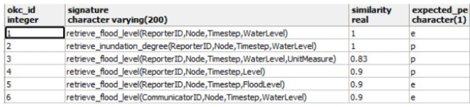
In order to simulate an open peer-to-peer environment, we created six different OKCs, each of them with a specific signature, similarity score,

(25)

Figure 8: Constraint to be solved by the sensor peer

and expected perf ormace. In this way, we simulated the real case in which a given peer can provide a service that is similar enough to what is required (defined by the LCC), but not exactly equal. Table 1 shows the OKCs defined for the selected e-Response scenario. Each OKC has a different signature; the similarity column shows the similarity score as computed by the matcher module of the OpenKnowledge kernel.

Table 1: Defined OKCs for the experiment

We have created two types of OKCs in order to simulate the case in which, even though a peer has a very high similarity score (and therefore a similar signature) but the implemented method does not perform exactly the same way as it is expected by the interaction model. The expected perf ormance column from Table 1 defines whether the OKC method will perform as speci-fied in the LCC (indicated by e), or not (indicated by p). In our experiments, by “performing as expected” we mean that the method should return the water-level value in meters. Therefore, we have a way to control the perfor-mance of the peer, from the point of view of the type of results the peer will be returning, independent of its actual behaviour (Correct or Incorrect). Using this structure we can define the overall result (water-level) of a sensor peer by the aggregation of the behavior and the expected performance of the OKC. The possible combinations are:

• Perfect sensor peer: a peer with correct behaviour (therefore not adding any error to the water-level), a perfect matching score and per-formanceas expected. This is the ideal case where the peer will give correct results.

• Good sensor peer: a peer with a correct behaviour, a matching score lower than 1, and performance as expected. This is the case where the peer will give correct results, even though it does not have a perfect matching score.

(26)

• Damaged sensor peer: a peer with incorrect behavior (e.g., because it’s damaged), and performance as expected. In this case the peer will be giving inaccurate results.

• Foreigner sensor peer: a peer with correct behavior, but with an OKC not performing as expected (poor performance p): for example, a peer using a different unit to the expected one; that is, instead of returning the correct results in meters (as expected), it returns them in inches, millimetres, etc. This case can be understood as if the peer has a correct behaviour (the water-level value is correct), but the peer “speaks a different language”, resulting in an overall inaccurate water-level value (in the sense the value is not what it was expected).

• Damaged foreigner sensor peer: a peer with incorrect behavior, plus it “speaks a different language”. Then the resulting value will be obviously inaccurate.

As can be seen in Table 1, we have defined three OKCs to have poor performance p. The transformations done for each of the poor performing OKCs are as follows considering their okc id:

• 2: The OKC returns the result in centimetres. • 3: The OKC returns the result in inches.

• 4: The OKC returns the water-level in relation to the sea-water-level, i.e., it adds 190 to the result, which is the height of the city of Trento above sea level.

In order to generate the peers for a given experiment, we have created a procedure that, given an experiment identifier (exp id), retrieves the corre-sponding behaviors and OKCs, and fills the sensor peer table automatically, creating the corresponding peers by considering the incidence of behaviours and OKCs. This means that it is relatively easy to create new settings to test the different characteristics of the several modules of the OpenKnowledge kernel, more specifically the Trust module, which is the aim of the current deliverable.

Annotations for the poll sensor interaction model

In order to enable the full capabilities of the matcher module over the constraints and variables of the LCC, we have annotated the variables related to the constraints in the reporter role (Figure 9). We have also annotated the message that will be used by the Trust module to compute the trust score. The message water level annotated as commitment represents the message that the peer under trust evaluation have to commit to, and therefore is used as input for the Trust module as defined in the Trust algorithm [1].

(27)

The constraint retrieve f lood level annotated to be memorised is used to asses the capability of a peer, i.e., how capable the peer is of satisfying the constraints for the role it is willing to play. The details on how trust is computed is out of the scope of this deliverable; for more details refer to Deliverable 4.5 and 4.8.

@annotation (@role (reporter) , @annotation (@variable(ReporterID), reporterID)) @annotation (@role (reporter) , @annotation (@variable(N ode), node))

@annotation (@role (reporter) , @annotation (@variable(T imestep), timestep)) @annotation (@role (reporter) , @annotation (@variable(W aterLevel), waterLevel)) @annotation(@role(reporter)

, @annotation(@message(water level(ReporterID, N ode, T imestep, W aterLevel)) , commitment(water level(ReporterID, N ode, T imestep, W aterLevel))))

@annotation(@role(reporter)

, @annotation(@constraint(retrieve f lood level(ReporterID, N ode, T imestep, W aterLevel) , memoize(retrieve f lood level( , , , ))))

Figure 9: Semantic annotations relative to the polling reporters interaction model

5.4.2 Running the experiment

In this section we present the configurations we have selected in order to run the experiments for the chosen e-Response test scenario.

Selected experiments configurations

We have defined 7 experiments in order to evaluate the selection strategies (Random, Trust and GEA) described in previous sections. We specified all the experiments in such a way that each node in the topology will have

at least one perfect or good sensor peer. By doing this, the worst case

scenario is that a node would have only one peer that will give correct results,

with all the other peers giving incorrect results. This means that, with

one of the informed selection strategies (based on information from previous interactions), the number of time steps needed to select a good peer is, in the worst case, the number of sensor peers in a node.

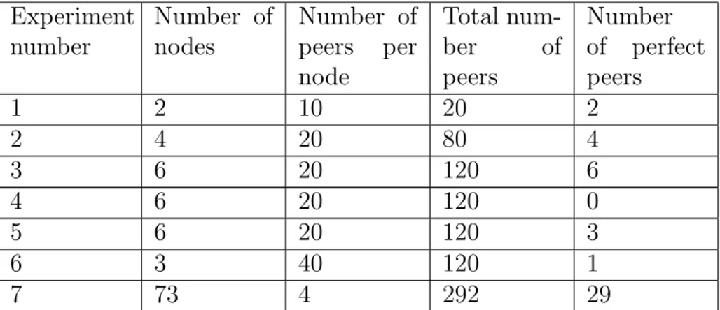
The rationale behind the definition of these experiments was to test how different variables impact on the quality of the results of the selection strate-gies. The variables being considered are the number of nodes, the number of peers per node, and the number of perfect peers per experiment.

Table 2 shows the values for the variables in each of the experiments. Experiments 1, 2, 3 and 7 are defined to evaluate the impact of an increasing number of nodes in the selection strategies. Experiments 1, 2, 6 and 7 are defined to study the effect of an increasing on the number of peers per node. Experiments 3, 4 and 5 are defined to study the impact of the distribution of perfect peers over the nodes, i.e., the cases when all the nodes have per-fect peers, some nodes have perper-fect peers, and no nodes have perper-fect peers.

(28)

Experiment number Number of nodes Number of peers per node Total num-ber of peers Number of perfect peers 1 2 10 20 2 2 4 20 80 4 3 6 20 120 6 4 6 20 120 0 5 6 20 120 3 6 3 40 120 1 7 73 4 292 29

Table 2: Defined experiments

Finally, Experiment 7 is the large scale experiment which tests the different modules of the OpenKnowledge kernel, using a large number of peers and all the nodes of the topology.

Experiment execution

The experiment execution consists of a single run of a selected configura-tion (experiment) of the chosen e-Response scenario. In order to launch the experiment we developed a java class (LaunchExperiment) that takes as in-put the experiment identifier (exp id) and the selection strategy we want to use for the run. The exp id is used to select the corresponding sensors from the database. For each selected sensor, a new instance of the OpenKnowl-edge kernel is then launched as a separate process. The necessary steps to run an experiment are the following:

1. Launch the discovery service (DS): the DS is the repository needed to store information about the available interaction models, and the peer subscriptions to these interaction models. For all the ex-periments, we initiate two instances of the discovery service in order to equally distribute the load given by the number of the peers.

2. Publish the interaction model: the poll sensor interaction model described in Section 5.3 is published. This is the interaction model used to define how peers (sensor peers and the Civil Protection Unit) interact with each other.

3. Launch the sensor peers for the experiment: the LaunchExperiment class is called with the experiment identifier. The class queries the database in order to get all the relevant peers, and spawns a new Open-Knowledge kernel for each one of the sensor peers needed. Each sensor peer subscribes then to the reporter role of the poll sensor interaction

(29)

model with a subscription description of the type ”reporter(nodeid)”, where nodeid denotes the node where the sensor is located.

4. Launch the Civil Protection Unit (CP U nit) peer: this sub-scribes to the querier role of the poll sensor interaction model with a subscription description of the type querier(all), After launching the CP U nit peer, all roles (querier and reporter) of the poll sensors in-teraction model will be fulfilled and, therefore, the inin-teraction model will be executed. The results of an experiment run are stored in the database for later analysis.

Since the necessary resources to run the different selection strategies were demanding, all the experiment runs were carried out in three dedicated servers at the University of Trento connected via a Gbit Ethernet LAN. The characteristics of the servers are:

1. 8 processors (Intel(R) Xeon(R) 2.50GHz); 16GB RAM

2. 2 processors (Dual-Core AMD Opteron(tm) 2.6GHz); 10GB RAM 3. 2 processors (Dual-Core AMD Opteron(tm) 2.6GHz); 9GB RAM

All the peers (CP U nit and sensors) plus the Discovery Service were distributively launched in these servers. In order to test the different modules of the OpenKnowledge kernel, we used this configuration to try as many capabilities during one single execution as possible, for example:

• Different instances of the Discovery Service were started in different servers, testing the distributed and load balancing capabilities of the DS.

• A large number of peers participated in the interaction model, which tested the ability of the Discovery Service to store their information, and the ability of the Coordinator to orchestrate the execution of the interaction model with many peers.

• The interaction model as defined in the LCC was complex enough to test several features of the LCC interpreter, such as recursion, annota-tions, etc.

• Peers for a given experiment were instantiated in different servers, test-ing the communication layer.

• Not all the peers had an OKC matching exactly the constraint in the interaction model: this tested the Matcher module and tested the open-world scenario where we may find similar but non-identical services to the ones we need.

• Peers with different OKCs had different behaviors (correct/incorrect): this tested the Trust module and its ability to identify peers with in-correct behaviours.

(30)

5.4.3 Experimental results

The aim of the experiments was to test the different selection strategies al-ready defined in the previous chapters. Here we summarise the three selection strategies:

• Random: first all the peers are grouped by node and all the peers are given the same score, then a random peer is selected for each node. • Trust: first all the peers are grouped by node, then a trust score is

computed using information from previous interactions and the peer with the highest trust score is selected per node. If several peers have the same highest trust score, a random choice is made between them. • GEA: first all the peers are grouped by node, then a GEA score is

computed as the combination of the trust score and the matching score of the peer. The peer with the highest GEA score is selected at each node. If several peers have the same highest GEA score, a random choice is made between them.

In order to evaluate the results of a given selection strategy we defined a quality metric. We used the mean absolute error metric defined in equation 2. It measures how accurate a given selection strategy is in selecting peers with correct results.

errort = 1 n·( n X i=1 |ei|), (2)

where t denotes the time step, n denotes the number of nodes, and ei

is the error defined in equation 3. In Equation 3, water levelo denotes the

obtained water-level (i.e., the result given by a sensor peer), and water levelr

denotes the real water-level as given by the flood sub-simulator.

ei =

(

0.5 if (water levelo6= water levelr)

0 otherwise (3)

Note that ei is not defined as (water levelo− water levelr) as it is

usu-ally defined, since what we want to evaluate is how many correct peers were selected by the selection strategy, not the overall distance between

the real water-level value water levelr and the obtained water-level value

water levelo. Equation 3 allows us to normalise the difference. In

conclu-sion, we want to minimise the number of peers giving incorrect results. Results

(31)

For each one of the experiments defined in Table 2 we run the complete setting with three selection strategies: Random Selection, Trust, and GEA. For each of these selection strategies we run the experiment 15 times in order to get statistically significant results. All the figures that follow represent average results for the 15 runs, for each of the selection strategies.

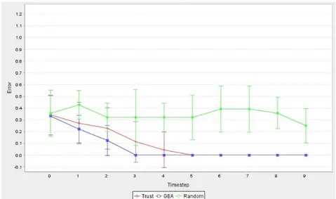
Figure 10: Mean absolute error for experiment 1. (2 nodes, 10 peers per node, 2 perfect peers)

Figure 10 shows the mean absolute error for experiment 1 as define in Table 2. The figure shows the results for the initial experiment, defined with two nodes and ten peers per node, and where all the nodes had at least one perfect peer. This initial experiment was carried out using only ten time steps in order to see the preliminary results of the Trust and GEA models. In the subsequent experiments the maximum number of time steps was set to 50. The initial results show that the selection strategies based on the use of information learnt in previous interactions improves peer selection. As we can see, the Trust based selection strategy is clearly better than the Random selection strategy. In this experiment configuration, GEA clearly outperforms the other two selections strategies. This means that in a setting where we have at least one perfect peer per node, GEA performs better than trust alone.

Figure 11 shows the result for Experiment 1 with the standard deviation σ. Let us define the following notation for the rest of the chapter. The

standard deviation for the Random selection strategy will be denoted by σR,

the standard deviation for the Trust selection strategy will be denoted by σT,

and the standard deviation for the GEA selection strategy will be denoted by

σG. We can observe from Figure 11 that, in general, σG is smaller than σT,

which in turn is smaller than σR. From σR we can infer that in some cases

(32)

does not remain constant, and, moreover, on average, the Random selection strategy selects bad peers.

Figure 11: Mean absolute error with standard deviation for experiment 1. (2 nodes, 10 peers per node, 2 perfect peers)

Figure 12 shows the results for Experiment 2. The rationale behind the definition of this experiment was to study the behavior of the selection strate-gies when we duplicate the number of nodes and the number of peers per node. Thus, Experiment 2 consists of 4 nodes with 20 peers per node, where each node has at least one perfect peer. As can be observed from Figure 12, increasing the number of nodes and peers does not change the general shape of the mean absolute error curves. The Random selection strategy has an average error of ∼0.5; the Trust selection strategy shows better results, but again is outperformed by GEA. From Figure 13 we can conclude that results

are statistically significant and that σT and σG decrease with time, while σR

remains approximately constant.

Figures 14 and 15 show the results for Experiment 3. In this experiment we wanted to test the impact of increasing the number of nodes over the selection strategies. As we can see from the figures bellow, the mean absolute error for all the selection strategies retain the same general characteristics as the ones for experiment 1 and 2 (Figures 10, 11, 12 and 13). We can conclude that an increase in the number of nodes does not affect the general behavior of the selection strategies.

Figures 16 and 17 show the results for Experiment 4. In the definition of this experiment we wanted to see the effect of not having a perfect peer in the nodes. In this experiment there are no peers with both perfect matching score and correct behaviour, but we do have incorrect behavior with perfect matching (damaged sensor peers). The experiment is meant to stress test the selection strategy and to study how the presence of such damaged sensor

(33)

peers affect their performance; would a given selection strategy be able to pin the peers down and discard them (by lowering their score) in the subsequent interactions?

As we can see from Figures 16 and 17, the Random and Trust selection strategies maintain the same behaviour, while the GEA selection strategy clearly changes the mean absolute error in the initial time steps. This change can be understood if we take into account that GEA uses matching informa-tion in order to select the peers. This means that, when there is no previous information (previous interactions with the peers), GEA will try to select

(34)

first those peers having higher matching score: all the bad peers (recall that in this experiment the peers with a perfect matching score have an incorrect behaviour). However, during the first time steps GEA learns (via Trust) how the selected peers behave incorrectly and, as a consequence, start to select peers from the second best matching score group. After some time steps, GEA finds the correct behaving peers and starts to select them, giving re-sults as good as the ones returned by Trust; finally in subsequent time steps, GEA even outperforms Trust.

(35)

Figure 16: Mean absolute error for experiment 4. (6 nodes, 20 peers per node, no perfect peer)

Figure 17: Mean absolute error with standard deviation for experiment 4. (6 nodes, 20 peers per node, no perfect peer)

We can conclude here that using Trust as selection strategy can be better than GEA in scenarios where we are not sure about the distribution of the types of peers among all the nodes.

Figures 18 and 19 show the results for Experiment 5. In this experiment we wanted to evaluate the case where 50% of the nodes had perfect peers. This experiment is set with six nodes, 20 peers per node, and three perfect peers, each assigned to different nodes. We can notice how the Random and Trust selection strategies have the same shape of the previous experiments. On the other hand, we can observe that the GEA results resemble the Trust

(36)

ones, being slightly worse at the beginning, but better after time step 7. We can infer that, on average, when half of the nodes have perfect peers, GEA and Trust performances are comparable.

Figures 20 and 21 show the results for Experiment 6. With this experi-ment we evaluated the performance of the Trust and GEA selection strategies when the number of peers per node is further increased. The experiment is set with 3 nodes, 40 peers per node and 1 perfect peer. We can deduce from

(37)

Figures 20 and 21 that the number of time steps taken by a given selec-tion strategy to have an average error of 0 is dependent on the number of peers they have to select. This observation might be intuitive, since, in the worst case, a selection strategy could first select all the peers giving incorrect results, and then select peers giving accurate results. By comparing these two Figures (20 and 21) with Figure 10 (experiment 1: 10 peers per node) and Figure 12 (experiment 2: 20 peers per node), it can be seen that in all the cases Trust and GEA selection strategies comply with the worst case expected results (i.e, the error is minimised to 0 in a time step that is less or equal than the total number of peers per node).

Figure 20: Mean absolute error for experiment 6. (3 nodes, 40 peers per node, 1 perfect peer)

In order to test the complete selected e-Response scenario, we have also defined an experiment with 73 nodes as provided in the e-Response evacua-tion scenario (experiment 7). In this case we defined only 4 peers per node, since we already showed how an increased number of peers per node does not affect the performance of both Trust and GEA selection strategies. The definition of the experiment ensure that all the nodes have at least one peer giving correct results, but does not necessarily ensure that all the nodes have perfect peers. In fact, only 29 nodes have perfect peers, approximately half of the nodes.

Figures 22 and 23 show the results for Experiment 7. The results given by Trust and GEA are very similar, again outperforming the Random selection strategy, which shows a trend similar to all the previous experiments. We can see also that both Trust and GEA have an error of zero in time step 3, which is less than the number of peers per node (4 peers per node for this experiment). This experiment demonstrates that both GEA and Trust give consistent results, even when the number of nodes increases.

(38)

Figure 21: Mean absolute error with standard deviation for experiment 6. (3 nodes, 40 peers per node, 1 perfect peer)

The results presented so far measure the outcome of the selection strate-gies according to the quality (mean absolute error) of the selection of the peers. An attempt to evaluate the selection strategies according to resource

usage was also made. We use the total computational time TT needed at

each time step in the interaction model as the metric resource. Such compu-tational time is composed by:

• TQ: Query time needed by the discovery service to retrieve the list of

(39)

all the time steps and the different selection strategies.

• TSel: Selection time needed by the selection strategies to group the

sensor peers per node, compute the scores and select the peer with

the highest score per node. TSel is highly dependent on the selection

strategy and is related to the time steps.

• TG: Group formation time needed by the coordinator to create a

mu-tually compatible group between all the subscribed peers of an inter-action model, in our case, all the sensors and the CP U nit. This time depends on the number of peers rather than the number of nodes, and remains constant throughout all the time steps and the different selec-tion strategies.

• TIM: Interaction model execution time. Once the peers that will

be participating in the interaction model are selected, the interaction model is executed at each time step. This time depends on the number of nodes, but remain constant throughout all the time steps and the different selection strategies.

Thus, TT is defined by Equation 4, where the time we want to evaluate is TSel

since is the variable time dependent on the currently used selection strategy.

TT = TQ+ TSel+ TG+ TIM (4)

Since we used three different servers as execution environments, it was