A stochastic approach to safety management of roadway segment

UNIVERSITY OF CATANIA

Faculty of Engineering

Department of Civil and Environmental Engineering

PhD Course on

“Engineering of Hydraulic Infrastructure,

Environmental Health and Transportation”

CYCLE XXVI

A STOCHASTIC APPROACH TO SAFETY

MANAGEMENT OF ROADWAY SEGMENT

CARMELO D’AGOSTINO

Supervisor:

Professor Salvatore Cafiso – University of Catania, Catania (IT)

Co-Supervisor:

Professor Bhagwant Persaud – Ryerson University, Toronto (CA)

Research Doctorate Coordinator:

Professor Salvatore Cafiso – University of Catania

SUMMARY

INTRODUCTION ... 5

Objectives of this Thesis and Overview of the Contents ... 13

CHAPTER 1 ... 17

SAFETY PERFORMANCE FUNCTIONs (SPFs): A GENERAL OVERVIEW ... 17

1.1. Introduction... 17

1.2. Literature overview... 18

1.2.1. Key points ... 52

1.3. Regression Technique, Model Form and Goodness of Fit Evaluation ... 53

1.4. Empirical Bayes Estimation and the Role of the NB Dispersion Parameter ... 62

1.5. Chapter summary ... 67

References ... 68

CHAPTER 2 ... 81

HOW TO ADDRESS THE TIME TREND EFFECTS IN THE CALIBRATION OF SPFs ... 81

2.1. Introduction... 81

2.2. The time correlation effects in the SPF ... 82

2.3. The Generalized Estimating Equation (GEE) methodology of calibration ... 84

2.4. Comparison between models with and without trend: a

case study ... 90

2.4.1, Data description and Models calibration ... 91

2.4.2. Results and model validation ... 94

2.5. Chapter summary ... 103

References ... 104

CHAPTER 3 ... 109

OPTIMIZATION OF THE GOF OF THE MODELS, VARYING THE SEGMENTATION APPROACH, FOR ROAD SAFETY SITE RANKING ... 109

3.1. Introduction ... 109

3.2. Methodological approach and literature review ... 111

3.3. Data gathering and treatment ... 113

3.4. Analysis and results... 117

3.4.1. Summary on the segmentation approach ... 134

3.5. Ranking of the road network ... 136

3.5.1. Empirical Bayes Ranking... 136

3.5.2. Potential for Safety Improvement (PSI) analysis ... 139

3.6. Chapter summary ... 143

References ... 144

CHAPTER 4 ... 149

CRASH MODIFICATION FACTOR AND FUNCTION ... 149

4.1. Introduction ... 149

4.2. Methodology ... 151

4.2.1. Before-after with comparison group analysis ... 154

4.2.3. Full Bayes before-after analysis ... 165

4.2.4. Cross sectional studies ... 168

4.3. Application of the Before-After EB to estimate a CMF for safety barrier meeting a new EU Standard: a case study.... 174

4.3.1. Segmentation approach and data treatment ... 181

4.3.2. Analysis and results ... 188

4.4. Crash Modification Function ... 197

4.4.1. Cluster analysis ... 199

4.4.2. Crash Modification Function calibration ... 204

4.5. Chapter summary ... 210

References ... 210

CHAPTER 5 ... 219

THE TRADITIONAL TECHNIQUES FOR THE BENEFIT-COST ANALYSIS AND THE CROSS SITE VARIANCE OF A CMF ... 219

5.1. Introduction... 219

5.2. The cost of crashes ... 221

5.3. Traditional techniques for the benefit-cost analysis .... 223

5.3.1. The net present value (NPV) ... 225

5.3.2. Benefit-Cost Ratio (BCR) ... 229

5.3.3. Cost-Effectiveness Index ... 230

5.4. The cross site variance of the CMF and CMFunction ... 231

5.5. Chapter summary ... 240

References ... 241

CHAPTER 6 ... 245

DEVELOPMENT OF A NEW STOCHASTIC APPROACH TO THE BENEFIT-COST ANALYSIS ... 245

6.1. Introduction ... 245

6.2. A stochastic approach to the Benefit-Cost analysis ... 246

6.2.1. Comparison between the deterministic and the stochastic Benefit-Cost analysis for existing infrastructures ... 253

6.2.3. Comparison between the deterministic and the stochastic Benefit-Cost analysis for new infrastructures ... 258

6.3. Montecarlo simulation for the Benefit-Cost analysis of a combination of CMFs ... 265

6.4. Chapter summary ... 270

References ... 271

SUMMARY AND CONCLUSIONS ... 275

INTRODUCTION

The targets of the thesis are road safety analysis based on crash event and road features for the benefit cost analysis where a treatment has to be applied.

There is a growing attention to road safety in Europe. New regulations applied on TERN network push Agencies to introduce new methodological approaches to Road Safety, monitoring the treatment and controlling the level of safety on the managed road network.

A crash is defined as a set of events that result in injury or fatality, due to the collision involving one motorized vehicle or a motor vehicle and another motorized vehicle, a bicyclist, a pedestrian or an object. The terms “crash”, “collision” and “accident” are typically used interchangeably.

“Crash frequency” is defined as the number of crashes occurring at a particular site, in a reference time period.

“Crash rate” is the number of crashes that occurs at a given site during a certain time period in relation to a particular measure of exposure (e.g., per million vehicle miles of travel for a roadway segment or per million entering vehicles for an intersection). Crash

rates may be interpreted as the probability (based on past events) of being involved in an accident per unit of the exposure measure.

Accidents count observed at a site (road segment, intersection, interchange) is commonly used as a fundamental indicator of safety performing road safety analysis methods.

Because crashes are random events, crash frequencies naturally fluctuate over time at any given site. The randomness of accident occurrence indicates that short term crash frequencies alone are not a reliable estimator of long-term crash frequency. If a three-year period of crashes were used as the sample to estimate crash frequency, it would be difficult to know if this three-year period represents a high, average, or low crash frequency at the site.

This year-to-year variability in crash frequencies adversely affects crash estimation based on crash data collected over short periods. The short-term average crash frequency may vary significantly from the long-term average crash frequency. This effect is magnified at study locations with low crash frequencies where changes due to variability in crash frequencies represent an even larger fluctuation relative to the expected average crash frequency.

The crash fluctuation over time makes it difficult to determine whether changes in the observed crash frequency are due to changes in site conditions or are due to natural fluctuations. When a period with a comparatively high crash frequency is

observed, it is statistically probable that the following period will be followed by a comparatively low crash frequency. This tendency is known as regression-to-the-mean (RTM), and also is evident when a low crash frequency period is followed by a higher crash frequency period.

Failure to account for the effects of RTM introduces the potential for “RTM bias”, also known as “selection bias”. Selection bias occurs when sites are selected for treatment based on short-term trends in observed crash frequency.

RTM bias can also result in the overestimation of the effectiveness of a treatment (i.e., the change in expected average crash frequency). Without accounting for RTM bias, it is not possible to know if an observed reduction in crashes is due to the treatment or if it would have occurred without the modification.

Another key analytical issue arises when accident rates are used in evaluating safety performance to, e.g., flag locations for safety investigation during the network screening process. AADTs are used directly in the computation of this measure, i.e., accident rate = accident frequency/AADT (or some scalar multiple of this). If accident rates are based on the observed counts, then the regression-to-the-mean difficulty discussed above will still apply. In addition, there is an additional problem that renders this method of screening dubious. The problem is that the relationship between accident frequency and AADT is not linear.

Specifically, comparing accident rates of two entities at different traffic levels to judge their relative safety may lead to erroneous conclusions and saying that when two rates are equal they indicate equivalent levels of hazard may be completely false if different AADT levels are involved.

Figure I.1 – Relationship between crash frequency and AADT

See Figure I.1 where two different curves (Curve1 and Curve2) are plotted to give an example. The two curves show the non linear relationship between entering AADT and the expected crash frequency, potentially for two different groups of intersections. It is clear that, in terms of crash rate (the slopes corresponding to each point of the curves), considering accident rates of points A and B, as well as A and C, to judge their relative safety, the comparison may lead to erroneous conclusions because

0,00 1,00 2,00 3,00 4,00 5,00 6,00 0 10 20 30 40 50 60 Exp ect ed N um ber o f I nj ur y C ol lisi on s/ Year

Average Entering AADT (Thousands)

B C Curve1 Curve2 A Points B and C Crash Rate Point A Crash Rate

points B or C could be considered by far safer than point A. Moreover, considering points B and C, the two corresponding rates are equal indicating equivalent levels of hazard, but this appears to be completely false because different AADT levels are involved.

The upshot of all this is that the use of accident rate to compare sites in regard to their safety levels is potentially problematic. When the slope of the accidents/AADT relationship is decreasing with increasing traffic volume levels, as is often the case, network screening by accident rates will tend to identify low AADT sites for further investigation. The most valid basis of comparison using accident rates is for the relatively rare cases when the traffic volume levels are the same or when the relationship between accidents and AADT is linear.

Conventional procedures for identifying sites for safety investigation tend to select sites with high accident counts and/or accident rates. However, accident counts could be high or low in a given period solely due to random fluctuations, leading to many sites either incorrectly identified or overlooked and, correspondingly, to an inefficient allocation of safety improvement resources. In addition, selection on the basis of accident rates tends to wrongly identify sites with low volumes. Empirical Bayes approaches have been proposed of late to overcome these difficulties.

The Highway Safety Manual (HSM) in its first edition (2010) introduced a new common approach to the modeling of crash analysis with the aims to standardize the methodology.

In its Part C the HSM provides a predictive method for estimating expected average crash frequency (including by crash severity and collision types) of a network, facility, or individual site. The estimate can be made for existing conditions, alternatives to existing conditions (e.g., proposed upgrades or treatments), or proposed new roadways. The predictive method is applied to a given time period, traffic volume, and constant geometric design characteristics of the roadway. The predictive method provides a quantitative measure of expected average crash frequency under both existing conditions and conditions which have not yet occurred. This allows proposed roadway conditions to be quantitatively assessed along with other considerations such as community needs, capacity, delay, cost, right-of-way, and environmental considerations. The predictive method can be used for evaluating and comparing the expected average crash frequency of situations like:

• Existing facilities under past or future traffic volumes;

• Alternative designs for an existing facility under past or future traffic volumes;

• Designs for a new facility under future (forecast) traffic volumes; • The estimated effectiveness of countermeasures after a period

• The estimated effectiveness of proposed countermeasures on an existing facility (prior to implementation).

Each chapter in Part C of HSM provides the detailed steps of the predictive method and the predictive models required to estimate the expected average crash frequency for a specific facility type like:

• Rural Two-Lane Two-Way Roads • Rural Multilane Highways • Urban and Suburban Arterials

However the application of the HSM doesn’t always provide adequate results in Europe (Cafiso et al. in 2012 applied the HSM methodology using data of a motorways in Italy in a study published on Procedia Elsevier - Social and Behavioral Sciences, titled “Application of Highway Safety Manual to Italian Divided Multilane Highways”, and Sacchi et al. in 2011 studied the transferability of the HSM models for intersection in Italy in a paper published on TRB titled “Assessing international transferability of the Highway Safety Manual crash prediction algorithm and its components”). The problem related to transferability of the Safety Performance Functions (SPFs) is a clear example of how the model developed in other Countries are not always able to catch the safety level of different infrastructures. The key point is that quantification of the expected reduction of crashes related to different treatments, can affect choices and plays a fundamental role in the decision making process. The transferability in HSM is

assessed using a factor of calibration to local condition. In this way using equation calibrated on “standard condition” and reported on the Manual, the application of the models in the whole North America is assessed. However many Authors have tried to apply HSM in Europe with poor results.

Together with SPFs the Highway Safety Manual introduced the “Crash Modification Factor” (CMF). A Crash Modification Factor is a multiplicative factor used to compute the expected number of crashes after implementing a given countermeasure at a specific site. The CMF is multiplied by the expected crash frequency without treatment. A CMF greater than 1.0 indicates an expected increase in crashes, while a value less than 1.0 indicates an expected reduction in crashes after implementation of a given countermeasure.

The best methodology of estimation of CMFs is well known to be based on stochastic approach. The problem of regression to the mean and the selection bias can be controlled using a sophisticated probabilistic approach reported in the “Observational Before/After Studies in Road Safety - Estimating the Effect of Highway and Traffic Engineering Measures on Road Safety” by Hauer in 1997 and developed by various author in the last 2 decades.

The new methodologies developed for the calibration of the Safety Performance Functions are pushing the Authors (See Persaud et al. “Comparison of empirical Bayes and full Bayes approaches for

before–after road safety evaluations” Published on Accident Analysis and Prevention in 2009) to find new advanced methodology able to address the problem of time trend and spatial correlation of data and to use more complicated model form and different distribution of outcomes in the calibration of CMFs. Despite the efforts on the calibration of CMFs to improve reliability, evaluation of safety benefits of applying a treatment continue to be performed using a deterministic approach. However in the HSM there is not a methodology to assess the CMFs transferability, and their stochastic nature doesn’t allow a perfect reliability also if they are applied in the same Country. Some Authors are developing different methodology to assess the transferability of the CMFs, and they should be applied when a CMF has to be used in a benefit cost analysis. The traditional techniques for the evaluation of the benefits of a treatment don’t take into account the statistical distribution of the CMFs and their stochastic nature.

Objectives of this Thesis and Overview of the Contents

The regression to the mean effect as well as the functional relationship between crashes and exposure factors don’t allow a reliable estimation of the effect of a treatment. Have a high reliability in the estimation of the effects of a countermeasures may be one of the most important issue in a Benefit-Cost analysis. The identification of hazardous location together with the evaluation of the alternatives to fix safety problem, are based on the reliability of the model used for the evaluation. For those reason the research

work provide a wide discussion on the main step for a reliable benefit-cost analysis starting from different methodology able to address the problem of regression to the mean and time trend effects and able to optimize the goodness of fit of the models varying the segmentation approach and the variables considered in the calibration of the models. The second step is to consider a new methodology for the evaluation of the variance of the CMFs. Particularly if a cross site variance is considered together with the variance of the CMF, as an indicator of the distribution of the CMF in different site, the perspective of considering the effect of a treatment can change drastically. The main objective of the present research work is to develop a methodology to perform Benefit-Cost analysis taking into account a cross site variability of the CMFs and their variance.

To do that an overview on the modeling approach is reported as well as a calibration of a Crash Modification Factor for safety barrier in Italy. At the end the proposed methodology for the stochastic benefit cost analysis is detailed described in comparison with the deterministic approach.

In the first Chapter an overview about SPFs is reported, with a wide literature review on the topic. In the second Chapter a methodology to address the time trend effects in the calibration of SPFs is applied using data on a motorways in Italy, the A18 Messina - Catania. Particularly the second Chapter focus on the problem of

time trend, generally presents when a long period of analysis is taken into account.

The third Chapter focuses on one of the possible method to optimize the model goodness of fit when roadway segment are analyzed. Particularly the segmentation approach was investigated and tested with the more common goodness of fit evaluation method. At the end of the Chapter a ranking was performed comparing the EB methodology to observed number of crashes and a methodology for the identification of hazardous location was applied.

In the fourth Chapter various methodologies to estimate a CMF are reported. As a case study an application of the empirical Babyes methodology is reported for the estimation of a CMF for road safety barrier. In the second part of the Chapter a Function was calibrated considering the functional relationship between the barrier direct related categories of crashes (ran-off-road crashes) and curvature using the same data of the presented case study.

The finals 5th and 6th Chapters deal with the benefit-cost analysis. The cross site variance was evaluated for the CMF calibrated in Chapter 4 and used in the stochastic benefit-cost analysis. A comparison on the traditional approach and a stochastic approach was performed for new and existing infrastructures. At the end of the Chapter a methodology to combine more CMFs in the same segment was described.

CHAPTER 1

SAFETY PERFORMANCE FUNCTIONs (SPFs):

A GENERAL OVERVIEW

1.1. Introduction

Road crash events are the object of many studies because of their potentially severe consequences. Thus, it is not a surprising that particular attention is given to the development of models able to identify features related to accidents and to forecast accident frequency.

Many researchers have developed accident prediction models also known as safety performance functions (SPFs) calibration. The high number of factors and the correspondingly high combinations of these factors related to accident event occurrence created need to develop different models for different circumstances. Models were developed specifically for urban and rural roads, for road segments and intersections; models account for different types of roads and intersections or even for different accident types and severity. Moreover, for the same safety performance function, the variables considered significantly related

to safety, as well as the statistical regression approaches adopted can vary considerably.

The statistical methodologies mainly adopted for calibration of safety performance functions, are the conventional linear regression and the generalized linear regression techniques. Since the mid-eighties, many research works highlighted the limitations of the conventional linear regression approach, which is why, nowadays the generalized linear regression technique (GLM) is the most common statistical regression methodology used. Nevertheless in the last two decades new techniques of calibration were carried out. One is the full Bayes methodology of calibration, which is able to account for the effect of regression to the mean and the Generalized Estimating Equation (GEE) able to account for the time correlation more extensive described in the Chapter 2. In the Present Chapter 1, a wide description of the model approach is reported with a literature review and the key points of the GLM methodology are explored, with particular attention to the reliability of the models.

1.2. Literature overview

Following, in chronological order, is a wide literature review regarding the statistical approaches adopted and results achieved by various studies and researchers. The literature overview starts from the early nineties and discusses in more depth the latest works dealing with the generalized linear modeling statistical regression technique. In general, the reviews merely summarize the

papers, including not only the approach and findings but also verbatim expressions of the authors’ opinions and beliefs and their own review of related work.

Review of Persaud and Dzbik (1993) [1.1]

These authors proposed a freeway accident modeling approach with the aim to overcome limitations of previous models.

In the authors’ opinion, the first difficulty with existing models is that they tend to be macroscopic in nature since they relate accident occurrence to average daily traffic (ADT) rather than to the specific flow at the time of accidents. Second, some modelers assume, a priori, that accidents are proportional to traffic volume and go on to use accident rate (accident per unit of traffic) as the dependent variable. There is much research to suggest that this assumption is not only incorrect but can also lead to paradoxical conclusions [1.2]. Third, conventional regression modeling assumes that the dependent variable has a normal error structure. For accident counts, which are discrete and nonnegative, this is clearly not the case; in fact, a negative binomial error structure has been shown to be more appropriate [1.3]. Finally, it is impossible for regression models to account for all of the factors that affect accident occurrence.

The need to overcome these difficulties was fundamental to the modeling approach adopted in the authors’ work. To this end, the authors adopted a generalized linear modeling statistical approach that allows the flexibility of a nonlinear accident-traffic

relationship and the possibility to choose a more appropriate error-structure for the dependent variable. The approach was applied to both microscopic data (hourly accidents and hourly traffic) and macroscopic data (yearly accident data and average daily traffic).

Generalized linear modeling using the GLM computer package was used to obtain a regression model for estimating P, the accident potential per kilometer per unit of time, given a freeway section’s physical characteristics, the volume (T) per unit of time, and a set of variables that describe operating conditions during the time period. The model form used was:

E(P) = a·Tb _(1.1)

where a and b are model parameters estimated by GLM. The macroscopic models were calibrated using data obtained from the Ontario Ministry of Transportation. For approximately 500 freeway sections, the accident count for the years 1988 and 1989 were used as an estimate of the dependant variable, and traffic data as an independent variable. To account for varying section lengths, the term log (section length) was specified as an “offset”, thus, in effect, models were estimated for prediction of the number of accidents per kilometer per year.

The microscopic models were calibrated using data pertaining to a 25-km segment of Highway 401 in Toronto, Canada. Part of this freeway, actually, has a Traffic Management System (FTMS) which provided detailed traffic data for short time periods.

separated by interchanges, and all have express and collector roadways typically with three lanes each per direction.

It was decided to disaggregate each day into 24 periods of 1 hour each and to derive data for each hour, for express and collector lane separately, and for day and night. For the accident data this task was straightforward. For the traffic data, it was necessary to derive hourly and seasonal variation factors and collector/express lane distribution factors and apply these factors to the average daily traffic. To maintain a reasonable level of homogeneity, only data pertaining to weekdays were used for the model calibration. After preliminary data analysis, it was decided to build the regression models using, for each section, only data for off-peak hours for which that section tended to be uncongested.

Figure 1.1 shows plots of the microscopic model regression prediction per kilometer per hour for two accident types (severe and total) and for express and collector roadways.

It is important to note that, for these regression lines, the slope is decreasing as hourly volume increases, perhaps capturing the influence of decreasing speed.

This is in contrast to the macroscopic plot in Figure 1.2, which all show increasing slopes. It is possible that the macroscopic plots are reflecting the increasing probability of risky maneuvers, such as passing and changing lanes, with higher ADT levels.

Figure 1.1. Microscopic regression model prediction

Review of Mountain, Fawaz and Jarrett (1996) [1.4]

These researchers developed and validated a method for predicting expected accidents on main roads with minor junctions where traffic counts on the minor approaches are not available.

The authors recognize that accidents at junctions are ideally modeled separately and that junction models do not normally assume a linear relationship between accidents and conflicting flows [1.5][1.6][1.7][1.8][1.9]. However, problems can arise because the application of such models requires, at a minimum, a knowledge of entry flows.

The data used for the study comprised details of highway characteristics, accidents and traffic flows in networks of main roads in seven UK counties for periods between 5 and 15 years. The networks represented a total of some 3800 km of highway. The road networks were restricted to UK A and B roads outside major conurbations. In addition to road type, the network roads were categorized according to carriageway type (single or dual) and speed limit (<40 mph (urban) and 40> mph (rural)). Junction accidents were defined as accidents occurring within 20 m of the extended kerblines of the junction.

The regression models were developed using the generalized linear modeling technique. This approach allowed a model form in which accidents are not linearly proportional related to traffic and the assumption of a negative binomial error structure for the dependent variable.

Results were compared with the COBA model (a basic model used in the U.K. for use in the cost benefit analysis), in which dependent variable is assumed to be proportional to the link length and traffic flow. It was clear that the proportional model used in COBA increasingly tended to overestimate the annual accidents as traffic volume increase. The non-linear model form showed that the linear model, as used in COBA, is inappropriate.

Review of Abdel-Aty and Radwan (2000) [1.10]

These authors argued that two major factors usually play an important role in traffic accident occurrence. The first is related to the driver, and the second is related to the roadway design.

Actually, as Abdel Aty et al. note, different researchers have attempted three approaches to relate accidents to geometric characteristics and traffic related explanatory variables: Multiple Linear regression, Poisson regression and Negative Binomial regression. However, recent research shows that multiple linear regression suffers some undesirable statistical properties when applied to accident analysis. To overcome the problems associated with multiple linear regression models, researchers proposed Poisson regression for modeling accident frequencies. They argued that Poisson regression is a superior alternative to conventional linear regression for applications related to highway safety. In addition, it could be used with generally smaller sample sizes than linear regression. Using the Poisson model necessitates that the mean and variance of the accident frequency variable (the

dependent variable) be equal. In most accident data, the variance of the accident frequency exceeds the mean and, in such case, the data would be over dispersed. Because of the over dispersion difficulties, the authors suggested the use of a more general probability distribution such as the Negative Binomial.

The primary objective of the Abdel-Aty and Radwan research was to develop a mathematical model that explains the relationship between the frequency of accidents and highway geometric and traffic characteristics. Other objectives include developing models of accident involvement for different gender and age groups using the Negative Binomial regression technique, based on previous research that showed significant differences in accident involvement between different gender and age groups [1.11][1.12][1.13].

In order to develop a mathematical model that correlates accident frequencies to the roadway geometric and traffic characteristics, Abdel Aty et al. argue that one needs to select a roadway that possess a wide variety of geometric and traffic characteristics. The goal of their data collection exercise was to divide the selected roadways into segments with homogenous characteristics. After reviewing several roadways in Central Florida, the authors decided that State Road 50 (SR 50) was most appropriate for this task. Information included geometric characteristics such as horizontal curves, shoulder widths, median widths, and traffic characteristics such as traffic volumes and speed

limits. SR 50 was divided into 566 highway segments defined by any change in the geometric and/or roadway variables. The data included the following variables: AADT, degree of horizontal curvature, shoulder type, divided/undivided, rural/urban classification, posted speed limit, number of lanes, road surface and shoulder types, and lane, median, and shoulder widths. Accident data were obtained from an electronic accident database for three years from 1992 to 1994.

The Poisson regression methodology was initially attempted. However, the Poisson distribution was rejected because the mean and variance of the dependent variables are different, indicating substantial over dispersion in the data. Such over dispersion suggested a Negative Binomial model to the authors who note that the Negative Binomial modeling approach is an extension of the Poisson regression methodology and allows the variance of the process to differ from the mean. The Negative Binomial model arises from the Poisson model by specifying:

lnli = bxi + e (1.2)

Where, li is the expected mean number of accidents on highway section i; b is the vector representing parameters to be estimated; xi is the vector representing the explanatory variables on highway segment i; e is the error term, where exp(e) has a gamma distribution with mean 1 and variance a2. The Negative Binomial model is calibrated by standard maximum likelihood methods. The

likelihood function is maximized to obtain coefficient estimates for a and b. The choice between the Negative Binomial model and the Poisson model can largely be determined by the statistical significance of the estimated coefficient a. If a is not significantly different from zero (as measured by t-statistics) the Negative Binomial model simply reduces to a Poisson regression.

In order to decide which subset of independent variables should be included in an accident estimation model, AIC (Akaike’s information criterion) was used by Abdel Aty et al. AIC identifies the best approximating model among a class of competing models with different numbers of parameters. AIC is defined as AIC=-2·ML+2·p, where ML is the maximum value of the log-likelihood function and p is the number of the variables in the model. The smaller the value of AIC, the better the model.

Two exposure variables were found to be significant. The first is the section’s length. The longer the length of the roadway section, the more likely accidents would occur on these sections. A similar conclusion was reached for the log of the AADT per lane. Moreover, the sharpness of the horizontal curve has a positive effect on the likelihood of accidents. Accidents increase with increasing degree of curve. An increase in shoulder width and median width was associated with a reduced frequency of accidents. There was an interaction effect between the lane width and the number of lanes. When the lane width increases, and at the same time the number of lanes decreases, the frequency of

accidents decline. Vertical alignment did not enter the model, possibly because Florida has relatively flat topography (i.e. little variation in slopes). Finally, the significance of the over dispersion parameter (a) indicates that the Negative Binomial formulation is preferred to the more restrictive Poisson formulation.

From the male and female accident involvement models, it could be concluded that female drivers experience higher probability of accidents than male drivers during heavy traffic volume and with reduced median width. Moreover, narrow lane width and larger number of lanes have more effect on accident involvement for female drivers than male drivers. Male drivers have greater tendency to be involved in accidents while speeding.

Young and older drivers have a larger possibility of accident involvement than middle aged drivers when experiencing heavy traffic volume. There is no effect of horizontal curve on older drivers’ accident involvement. Older age drivers, however, have a greater tendency to accident occurrence than middle and young drivers for reduced shoulder width and median widths. Decreasing lane width and increasing number of lanes creates more problems for older drivers and younger drivers than middle age drivers. Older drivers experience fewer accidents if the shoulder is paved. Also, the likelihood of younger drivers’ accident involvement increases with speeding.

Review of Garber and Ehrhart (2000) [1.14]

This study identified the speed, flow, and geometric characteristics that significantly affect crash rate and developed mathematical relationships to describe the combined effect of these factors on the crash rate for two-lane highways.

The authors noted that previous research of crash rates and hourly traffic volume revealed a U-shaped relationship, indicating that higher crash rates are observed during the early-morning and late-day hours when the traffic volume is low [1.15][1.16]. This has been further extrapolated to conclude that, as the number of vehicles on the highway increases, the variation between vehicle speeds decreases and that it is the speed variance that affects the crash rate [1.17][1.18][1.19]. The type of crash also has been shown to be a function of the traffic volume. The percentage of multiple-vehicle crashes decreases as the traffic volume decreases, and the percentage of single-vehicle crashes increases with a decrease in volume [1.20].

Garber et al. cited research showing that a U-shaped relationship exists between the probability of a vehicle being involved in a crash and the deviation of the vehicle’s speed from the mean speed of the traffic. This relationship indicates that the greater a vehicle speed deviates from the mean speed, the greater is the probability of that vehicle being involved in a crash [1.20]. This implies that driving both slower and faster than the mean

speed increases the likelihood of being involved in a crash, according to Garber et al.

The review by Garber et al. found that the main geometric characteristics that have been found to influence safety for two-lane roads are two-lane width and shoulder width. The results obtained from these studies have tended to be inconsistent. A few studies also have investigated the effect of grade on crashes for two-lane highways. Although it is generally accepted that grades of 4 percent or lower have an insignificant effect on crashes, the results of these studies also have been contradictory.

In the actual Garber and Ehrhart (2000) research, data collection consisted of obtaining speed, flow, and crash data for the road segments selected for the study and defining roadway characteristics, such as the number of lanes, for the segments. Lengths of the roadway segments were identified between traffic monitoring stations, positioned on major intersections, to ensure homogeneous traffic and flow characteristics.

The modeling process began with the use of the independent variables mean speed (MEAN), standard deviation of speed (SD), flow per lane (FPL), lane width (LW), and shoulder width (SW), and with crash rate (CRASHRATE) as the dependent variable. Two deterministic modeling procedures (multiple linear regression and multivariate ratio of polynomials) were applied to the data in search of an adequate fit, but in the end, multivariate

ratio of polynomial models seemed to better described the relationship between the dependent and independent variables.

The authors recognized that once models have been constructed, a suitable measurement of quality must be applied to select the model that best fits the observed data. Two such measurements were applied in this research: the coefficient of determination (R2_{) and Akaike’s information criterion (AIC).}

The R2 _{value is a popular measure used to judge the} adequacy of a regression model. Defined as a ratio, the R2 _{value is a} proportion that represents the variability of the dependent variable that is explained by the model. In symbolic form:

(

)

(

)

∑

∑

y : mean of the observations yi: actual observations

An R2 _{value near zero indicates that there is no linear} relationship between the dependent and independent variables, while a value near 1 indicates a linear fit. The authors note that the R2 _{value should be used with caution to ensure its correct} interpretation, and it always should be accompanied by an examination of the residual scatter plots; also, that the R2 _{value is} not an appropriate measure for nonlinear regression because its purpose is to measure the strength of the linear component of the

model. Therefore, another method must be introduced to compare the multivariate models. The method chosen was the AIC, which was developed as a means to predict the fit of a model based on the expected log likelihood.

The results of this research established that the crash rate is not linearly related to speed, flow, and geometric characteristics. Of all of the independent variables considered in this study, the standard deviation of speed (SD) seemed to have the greatest impact on the crash rates for two-lane highways.

Review of Pardillo and Llamas (2003) [1.21]

These researchers developed a set of multivariate regression models to estimate crash rates for two-lane rural roads, using information on accident experience, traffic and infrastructure characteristics. The research includes identifying relevant variables, model calibration and precision analysis of the method for accident rate prediction and for assessment of road safety improvement projects effectiveness. In the development of accident prediction models two key questions have to be solved, as the authors note: functional model form choice and independent variable selection.

The authors felt that in recent years, there was a consensus among researchers in favor of modelling accidents as discrete, rare, independent events, usually as generalized linear Poisson models in which the frequency of crashes that occurs in a given road section is treated as a random variable that takes discrete integer non-negative values. A characteristic feature of the distribution is

that the variance of the variable is equal to its mean. The mean number of accidents is assumed to be an exponential applied to a suitable linear combination of road variables. The resulting models are generalized linear models (GLIM), in which the exponential function guarantees that the mean is positive. The authors cited Maher and Summersgill [1.22] who developed a comprehensive methodology to fit predictive accident models applying this approach.

In 1994 Miaou [1.23] introduced negative binomial models, a generalization of the Poisson form that allows the variance to be over-dispersed and equal to the mean plus a quadratic term in this mean whose coefficient is called the overdispersion parameter. When this parameter is zero, a Poisson model results.

Vogts and Bared [1.24] developed a series of Poisson and Negative Binomial multivariate regression models to predict accident frequencies in 2-lane rural roads and intersections. Prediction variables in non-intersection models include traffic volume, commercial vehicles percentage, lane and shoulder width, horizontal and vertical alignment, road side condition and driveway density.

Independent variable selection for accident prediction models remains a complicated problem. Krammes et al. [1.25] and Lamm et al. [1.26] have both shown with their works the importance of taking into account design consistency when considering safety effects of highway characteristics on crash risk.

A sample 3450 km of two-lane rural roads was used in this research. Crash data was obtained and analyzed in two periods: 1993-97 and 1998-99. The first period was used in model calibrations, while the second period was reserved to assess model accuracy. Traffic and roadway characteristics dataset contains one record every 10 m of roadway including the following data:

• AADT (veh/day) • Curvature(m-1₎

• Longitudinal grade (%) • Roadway width (m) • Right shoulder width (m) • Left shoulder width (m) • Sight distance (m) • Access points

• Posted speed limit (km/h) • No passing zones

• Safety barriers

Dividing the sample in homogeneous sections in which all the characteristics of the highway were constant resulted in segments with of an average length of less than 400 m. Previously, in 1997, Resende and Benekohal [1.27] had reached the conclusion that to get reliable accident prediction models crash rates should be computed from 0.8 km or longer sections. It was decided that the average length of homogeneous sections was too short to allow for a meaningful analysis of the effect of potential roadway

improvements on safety. For that reason, the study was conducted in parallel for two types of sections. For the first one the 3450 km sample was divided in 1 km fixed length segments. For the second, the same sample was divided into 236 highway sectors or sections of variable length limited by major intersections and/or built-up areas within which traffic volumes and characteristics could be assumed to be constant. The length of these highway sectors ranged between 3 km and 25 km, with an average of 14.6 km.

The variables that were considered in the analysis for the 1 km long segments were:

• Access density (access points/km) • Average roadway width (m) • Minimum sight distance (m) • Minimum curvature (1/m) • Minimum speed limit (km/h)

• Maximum grade in absolute value (%) • Minimum design speed (km/h)

• Design speed reduction from the adjacent 1 km segments (km/h)

The variables that were considered in the analysis for the highway sectors or sections of variable length were:

• Access density (access points /km ) • Average roadway width (m)

• Average sight distance (m) • Average curvature (1/m)

• Standard deviation of curvature (1/m) • Average speed limit (km/h)

• Maximum longitudinal grade (%)

• Average of the absolute values of grade (%) • Average design speed (km/h)

• Standard deviation of design speed values (km/h)

• Average design speed variation between the 1 km long adjacent segments included in the sector (km/h)

• Proportion of no passing zones

Independent variable selection was performed with the objective of identifying those variables that show higher degree of association with crash rates. Traffic volume was found to be the variable with the highest correlation with crash frequencies.

In 1 km segments, the highest correlation coefficients with the average accident rate for the study period were:

• Access density (access points/km)

• Design speed reduction from adjacent segments (km/h) • Speed limit (km/h)

• Average sight distance

When longer sections were considered, the highest correlation coefficients with the average accident rate were:

• Access density (access points/km) • Average speed limit (km/h) • Average sight distance (m)

From the results of the research performed by Pardillo and Llamas, the following conclusions were obtained:

• A key step to develop accident prediction models is to select a set of independent variables that capture as much of the interaction between roadway characteristics and driver safety performance as possible. To do this a univariate correlation analysis can be conducted prior to the calibration of multivariate models.

• The highway variables that have the highest correlation with crash rates in Spain´s two-lane rural roads are: Access density, average sight distance, average speed limit and the proportion of no-passing zones. Access density is the variable that influences most the rate of head-on and lateral collisions, while in run-off the road and single vehicle crashes sight distance is decisive. • High access density has a negative effect on safety.

Therefore preventive safety improvements should include access management and control measures.

• To measure the influence of geometric design on crash rates it is necessary to use variables that measure the variation of characteristics between adjacent alignment elements or along a highway section. This confirms the importance of achieving highway design consistency to improve safety.

Review of Ng and Sayed (2004) [1.28]

The objectives of this study were to investigate and quantify the relationship between design consistency and road safety.

Design consistency is the conformance of geometry of a highway with driver expectancy, and its importance and significant contribution to road safety is justified by understanding the driver– vehicle–roadway interaction. When an inconsistency exists that violates driver’s expectation, the driver may adopt an inappropriate speed or inappropriate maneuver, potentially leading to accidents. In contrast, when design consistency is ensured, all abrupt changes in geometric features for continuous highway elements are eliminated, preventing critical driving maneuvers and minimizing accident risk (Fitzpatrick and Collins 2000) [1.29].

Currently, several measures of design consistency have been identified in the literature and models have been developed to estimate these measures. These measures can be classified into four main categories: operating speed, vehicle stability, alignment indices, and driver workload.

Operating speed is a common and simple measure of design consistency. Operating speed is defined as the speed selected by the drivers when not restricted by other users, i.e., under free flow conditions, and it is normally represented by the 85th _percentile speed, denoted as V85 (Poe et al. 1996) [1.30]. The difference between operating speed and design speed (V85-Vd) is a good indicator of the inconsistency at one single element, while the

speed reduction between two successive elements (ΔV85) indicates the inconsistency experienced by drivers when traveling from one element to the next. Lamm et al. (1999) [1.31] have established consistency evaluation criteria for these measures.

Many models have been developed to determine operating speed in terms of alignment parameters. Morrall and Talarico (1994) [1.32] have related V85 (kilometers per hour) on horizontal curves to the degree of curve DC using data on two-lane rural highways in Alberta.

Lamm et al. (1999) have suggested that another measure that can account for more variability of operating speed on curves is the curvature change rate CCRs because it takes transition curves into consideration, as shown below

(1.4)

where CCRs is measured in gon per kilometers (gon is a designation of the angular unit (1 gon = 0.9°)), Lcr is the length of circular curve (meters), Lcl1 and Lcl2 are the lengths of spirals preceding and succeeding the circular curve (meters), and L = Lcr + Lcl1 + Lcl2 is the total length of curve and spirals (meters).

Operating speed on tangents connecting horizontal curves of an alignment is also important for design consistency evaluation. Tangent length is one of the factors that determines the necessary

speed reduction when entering a horizontal curve and forms the basis of the definitions of dependent and independent tangents. An independent tangent is a tangent that is long enough to allow drivers to reach their desired operating speed, and consequently a speed reduction of greater than 20 km/h is required when they enter the following curve (Lamm et al. 1999). In contrast, a nonindependent tangent is one that is not long enough, and therefore a speed reduction that is greater than 20 km/h is not required. Speed on nonindependent tangents is less complex to model than that on independent tangents that generally depend on a whole array of roadway character. Some research has been undertaken to model operating speed on independent tangents, but the results are considered preliminary (Polus et al. 2000) [1.33].

Alignment indices are defined as quantitative measures of the general character of an alignment. They reveal geometric inconsistencies when the general characteristics of the alignment change significantly. While speed reduction and vehicle stability are good measures of design consistency, they are symptoms rather than causes. It is the geometric design itself, or specifically, the geometric characteristics and the combinations of tangents and horizontal curves that create inconsistencies. One of the indicators of geometric inconsistency is a large difference between the value of an alignment index of an individual feature and the average value of the alignment. The ratio of the radius of an individual horizontal curve to the average radius of the alignment (roadway

section), denoted by CRR, is adopted in Ng and Sayed research work.

Driver workload can be defined as the time rate at which drivers must perform the driving task that changes continuously until it is completed (Messer 1980) [1.34]. Conceptually, driver workload can be a more appealing approach for identifying inconsistencies than operating speed because it represents the demands placed on the driver by the roadway, while operating speed is only one of the observable outputs of the driving task. However, the use of driver workload is much more limited than operating speed because of its subjective nature (Krammes and Glascock 1992) [1.35].

Two measures have been proposed in the literature to measure driver workload, namely sight distance and visual demand. Limited sight distance increases driver workload as the driver needs to update his information more frequently and process it more quickly. However, little research has been conducted to investigate the relationship between driver workload and sight distance. In contrast, a number of studies have been carried out to examine the potential of visual demand as a measure of driver workload. Visual demand is defined as the amount of visual information needed by the driver to maintain an acceptable path on the roadway (Wooldridge et al. 2000) [1.36].

The models developed to estimate visual demand of unfamiliar drivers (VDLU) and visual demand of familiar drivers

(VDLF) were found to be inversely proportional to horizontal radius, meaning that driver workload increases with a decrease in radius [1.37].

The study conducted by Ng and Sayed uses geometric design, accident, and traffic volume data recorded on a two-lane rural highway. Specifically, accidents that occurred within 50 m of signalized intersections or within 20 m of all other types of intersections were eliminated. The design consistency measures mentioned previously, namely V85-Vd, ΔV85, CRR, VDLU, and VDLF, were computed for each section. The data included 319 horizontal curves and 511 tangents.

The methodology used in this study is based on the development of Accident Prediction Models incorporating design consistency measures. The models are developed using the generalized linear regression modeling (GLM) approach. The following model form was adopted:

(1.5) where E(Λ) is the expected accident frequency; L is the section length; V is the annual average daily traffic (AADT); xj is any

of the m variables in addition to L and V; and a0, a1, a2, and bj are

model parameters. The error structure of the models is assumed to follow the negative binomial distribution.

Models developed showed accident frequency to be positively correlated to V85-Vd, ΔV85, VDLU, and VDLF, and is negatively correlated CRR.

A qualitative comparison was also made to compare accident prediction models that explicitly consider design consistency with those that rely on geometric design characteristics for predicting accident occurrence. The comparison, while limited to fictitious alignments and not real data, shows that the first type may be superior as it can potentially locate more inconsistencies and reflect the resulting effect on accident potential more accurately than the second. The prediction accuracy of accident prediction models is limited by the quality of their independent variables. As such, the models developed in this study depend heavily on the design consistency measures used.

Review of Zhang and Ivan (2005) [1.38]

These researchers used Negative Binomial (NB) Generalized Linear Models (GLIM) to evaluate the effects of roadway geometric features on the incidence of head-on crashes on two-lane rural roads in Connecticut.

Many previous studies have applied NB GLIM in highway crash analysis under different circumstances. Wang and Nihan (2004) [1.39] used NB GLIM to estimate bicycle-motor vehicle (BMV) crashes at intersections in the Tokyo metropolitan area. Shankar et al. (1995) [1.40] also adopted NB GLIM in modeling the effects of roadway geometric and environmental features on

freeway safety. Miaou (1994) [1.41] evaluated the performance of negative binomial regression models in establishing the relationship between truck crash and geometry design of road segments.

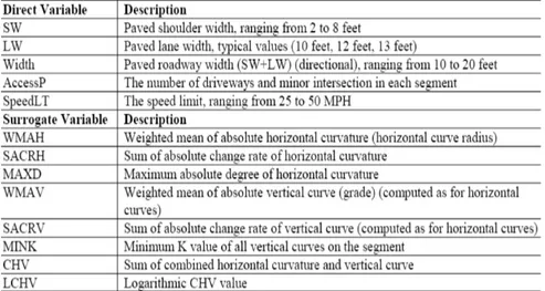
For Zhang and Ivan research, six hundred fifty-five segments, each with a uniform length of one kilometer, were selected from fifty Connecticut state-maintained two-lane rural highways. The selection was based on the land use pattern, permitting only minor intersections (without signal or stop control on the major approaches) and driveways along the segments. Information concerning speed limit, clear roadway width, number of driveways and minor intersections, and geometric characteristics such as the horizontal curvature and the vertical grade were collected. The definitions of the selected variables are shown in Table 1.1.

Table 1.1. Definition of Site Characteristic Variables (Zhang and Ivan, 2005)

The Akaike's Information Criterion (AIC) [1.42][1.43] was used for selecting the best of the models and to highlight variables significantly related to safety. Four of the site variables were found to be significant at 95 percent confidence for predicting the head-on crash count: SACRH, SACRV, MAXD, and SpeedLT (speed limit). Moreover, the authors found that the coefficient for the natural log of AADT is significantly different from 0, rejecting the hypothesis that the rate of head-on crashes is constant with volume. This coefficient is actually negative, suggesting a decreasing trend for on crash rate with AADT. This was not expected, since head-on crashes are expected to occur more often at higher volumes than at lower volumes, as drivers would have more opportunities to conflict with vehicles approaching from the opposite direction. Nevertheless, since head-on collisions are so rare, this relationship may be relatively weak. Also, drivers may pay more attention to safety when they see more traffic coming from the opposite direction, thus reducing the rate of head-on crashes at high traffic volumes.

Consistency of geometric design can be approached in two ways. Some studies have analyzed lengths of road, to address the possibility that accidents may not occur at “the most inconsistent” element (curve or tangent) of the alignment but somewhere within a road section of poor consistency. The more usual approach is to analyze individual elements (curves and tangents) of the alignment. This provides a more specific level of analysis.

Review of Bird and Hashim (2006) [1.44]

A similar approach to Zhang and Ivan was adopted in this research in which authors aimed to find whether relationships could be found between accident locations and various consistency measures at element level. Many consistency variables were defined for this study, some have been used before in other studies, and some were new ones defined by the authors for this particular study. These variables can be alignment indices (ratio of curve radius to average curve radius) or speed indices (difference between operating speed on an element and speed limit).

Other research has been carried out to develop accident prediction models that are based on a range of alignment consistency measures. Anderson (1999) [1.45] developed several regression models to relate the accident frequency to 5 different consistency measures separately. These measures include operating speed reduction, average radius, ratio of an individual radius to average radius and average rate of vertical curvature. His data set consisted of 5287 horizontal curves in 6 states in USA. His final conclusion stated these four consistency measures appeared suitable for assessing the safety of highways. The fifth measure, ratio of maximum to minimum radius on a roadway section, was found not to be as sensitive to predicted accident frequency, and was therefore not recommended as a design consistency measure. Other work on Canadian roads, recently reported by Hassan et al. (2005) [1.46], found that operating speed consistency provided

superior models in relation to collision frequency than design-speed margin consistency.

The research proposed by Bird and Hashim (2006), was based on a sample of 380 km of rural single carriageways (two lane undivided highways). Sections in built up areas (villages or towns) or near (within 20 meters of) junctions with other A or B class roads were excluded. The study required geometric details of each element of the alignment of the road, thus alignment characteristics (e.g. length of element, radius, deflection angle and degree of curve) were collected. The final sample contained 620 curves and 594 tangents. The study considers only personal injury accidents (PIA) because in the U. K., only personal injury accidents must, by law, be reported to the police. The time period for the accident data was 2000-2004. Accident records were allocated to the correct elements (e.g. curve or tangent) using the easting and northing coordinates of each accident and element.

One of the variables used in calculating some of the consistency measures is operating (85th percentile) speed. The design speed was also used as part of some consistency indices.

So as already highlighted previously, the technique of Generalized Linear Modelling (GLM) offers a suitable and sound approach for developing accident prediction models. The general form of the accident prediction model is therefore:

where:

m = estimated accident frequency L = section length

AADT = section average annual daily traffic, Xj = any additional variables

β0, and βj = the regression parameters

The usual test for goodness of fit for standard regression analysis is the R2 value. However this has shortcomings when used in accident analysis as stated by Miaou (1995) [1.47]. Many other measures have been suggested by Miaou and other authors [1.48][1.49][1.50]. Miaou suggested using the negative binomial overdispersion parameter k to determine how well the variance of data is explained in a relative sense. This is expressed as:

k k

Rk2 =1− max (1.7)

where

k = estimated overdispersion parameter for the chosen model

kmax= the estimated overdispersion parameter for a model with only an intercept term.

Two other measures can be also used, the mean scaled deviance and the mean Pearson χ2.

Taking up Bird and Hashim study again, before accident prediction models were created, it was necessary to define the individual variables to use in the analysis. Two main exposure variables were used, the length of the element, and the traffic flow on it. Other variables fell into two groups, direct geometric variables, and speed and consistency indices.

The first stage of the study involved the development of models for groups of accidents, for curves, tangents and then for the combined dataset. For all the models calibrated, side access density (direct variable) and the absolute difference between the speed limit and element operating speed (consistency variable), was found to be statistically significant.

Review of Polus and Mattar-Habib (2004) [2.51]

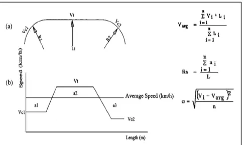
These authors utilized operating speed profiles on nine two-lane rural roads segments having lengths ranging from 3 to 10 km each in northern Israel. Two measures of consistency were developed for these segments. The first measure was the normalized relative area (per unit length), bounded between the speed profile and the average speed line. The average operating speed, Vavg, was computed as the average weighted speed, by length, along the entire segment. If the areas bounded between the speed profile and the average operating speed line are denoted by ai, as shown in Figure 1.3, then the first consistency measure is

(1.8)

Where Ra is the relative area (m/s) measure of consistency; ∑ai is the sum of areas bounded between the speed profile and the

average operating speed (m2_{/s); and L is the entire segment length.} The second measure of consistency was the standard deviation of speed (s) along the road segment. The standard deviation is the most appropriate statistical measure of data distribution around the mean value. It was necessary to use this additional measure to complement the first measure because the Ra measure by itself provided similar result for somewhat different geometric characteristics in a few cases, though this was rare.

Figure 1.3. (a) Example of road section and (b) example of speed profile

The standard deviation of the operating speed was defined as:

s = [(Vi – Vavg)2/n]0.5 (1.9)

where s is the standard deviation of the operating speeds (km/h); Vi is the operating speed along the ith geometric element (tangent or curve) (km/h); Vavg is the average weighted (by length) operating speed along a road segment (km/h); and n is the number of geometric elements along a section (km/h).

These two measures of consistency provide an independent assessment of the resemblance (i.e., consistency) of speed performance along the entire road segment under study. Their main advantage is that they consider the consistency of the overall longitudinal segments, not just individual speed differentials between two successive elements.

As the relative weighted area bounded by the speed profile and the average weighted operating speed increases, so does the inconsistency of speeds. The standard deviation of operating speed also increases as the distribution becomes more dispersed. These two measures were found, opportunely combined in a road safety evaluation model developed by authors, significantly related to safety.

1.2.1. Key points

On the basis of the literature review presented so far, some key points need to be emphasized regarding statistical accident modelling for motorways, the focus of this thesis.

First, the generalized linear modelling technique (GLM) is appropriate for safety performance function calibration. This approach overcomes the limitations of conventional linear regression in accident frequency modeling, and allows a Poisson or Negative Binomial error structure, distributions that are more pertinent to accident frequency modelling, to be assumed. Together with this, new techniques of calibration can be used.

Second, the model form adopted has to account for the nonlinear relationship between accident frequency estimate and traffic volume variable; moreover it has to allow for the dependent variable to logically equal zero as the exposure variables goes to zero.

Third the independent variable definition and selection must account for road geometric features as well as consistency measures and road context-related characteristics.

Fourth, in parallel with the independent variable choice issue, the state of the art analysis revealed research focusing also on providing guidelines or suggestions to define and obtain homogeneous segments [1.10][1.14][1.21][1.38][1.51]. Cafiso et al. [1.52] also presented a detailed methodology purposely set up for

dividing the entire path into segments characterized by homogeneous highway features related to safety.

On the basis of the literature review, and in order to organize the concepts relevant to this thesis, following is summarizes descriptions of the statistical regression technique used for safety performance function calibration, the choice of model form, and the most frequently used goodness of fit measures for safety performance function evaluation.

1.3. Regression Technique, Model Form and

Goodness of Fit Evaluation

In the first instance a note on terminology is needed to clarify some terms used in the following chapters. The term accident prediction models, often used to indicate safety performance functions, usually denotes a multivariate model fitted to accident data in order to estimate the statistical relationship between the number of accidents and factors that are believed to be related to accident occurrence. The term “predictive” is somewhat misleading; “explanatory” would be a better term. Prediction refers to attempts to forecast events that are yet to occur, whereas accident prediction models are always fitted to historical data and can thus only describe, and perhaps explain, past events [1.53].

Moreover, the choice of the explanatory variables potentially affecting the safety performance of a site ought to be based on theory [1.54]. A theoretical basis for choosing explanatory

variables might take the form of, for example, a causal model [1.55]. In practice, a theoretical basis for identifying explanatory variables is rarely stated explicitly [1.56]. The usual basis for choosing explanatory variables appears to be simply data availability. It is obvious that any analysis will be constrained by data availability. Nevertheless, the choice of explanatory variables should ideally not be based on data availability exclusively. Explanatory variables should include variables that:

• Have been focused in previous studies to exert a major influence on the number of accident;

• Can be measured in a valid and reliable way;

• Are not endogeneous, that is dependent on other explanatory variables included or on the dependent variable in the model.

Historically, two statistical modeling methods have been used to develop collision prediction models: conventional linear regression and generalized linear regression [1.57]. Recently however, generalized linear regression modeling (GLM) has been used almost exclusively for the development of collision prediction models. Several researchers (e.g. Jovanis and Chang 1986, Hauer et al. 1988, Miaou and Lum 1993) [1.58][1.9][1.59] have demonstrated the inappropriateness of conventional linear regression for modeling discrete, non-negative, and rare events such as traffic collisions. These researchers demonstrated that the standard conditions under which conventional linear regression is appropriate (Normal model errors, constant error variance, and the