INEA 2013
edited by Flavio Lupia
A ModeL-bAsed irrigAtion
wAter consuMption estiMAtion
At FArM LeveL
Istituto Nazionale di Economia Agraria
A Model-bAsed irrigAtion
wAter consuMption estiMAtion
At fArM level
edited by Flavio Lupia
Editor: Flavio Lupia Contributors:
INEA
Flavio Lupia - Foreword, Introduction, Glossary, Annex 1, Chapter 5, Paragraphs: 2.4,
3.4.2, 4.1, 4.2, 4.3, 4.4 and 4.5
Silvia Vanino - Paragraphs 3.2 and 3.3
Francesco De Santis - Annex 1, Paragraphs: 2.4, 4.1, 4.2 and 4.3 Filiberto Altobelli - Paragraph 2.5
Giuseppe Barberio - Chapter 5 Pasquale Nino - Paragraph 2.6 ISTAT
Giampaola Bellini - Chapter 1
Giancarlo Carbonetti - Paragraph 4.1 Massimo Greco - Paragraph 3.1 Luca Salvati - Paragraph 3.4.1 IAS-CSIC
Luciano Mateos - Paragraphs: 2.1, 2.2, 2.3, 2.4 and 4.2 CRA-CMA
Luigi Perini - Paragraph 3.4.3 Free-lance consultants
Nicola Laruccia - Paragraph 3.3 Disclaimer:
“This publication has been realized in the framework of the MARSALa project funded by Eurostat with the Grant Agreement No. 40701.2008.001008.140 (Grant Programme 2008 - Theme “Pilot studies for estimating the volume of water used for irrigation”). Its content does not represent the official position of the European Commission and is entirely under the responsibility of the authors.”
“The information in this document is provided as is and no guarantee or warranty is given that the information is fit for any particular purpose. The user thereof uses the information at its sole risk and liability.”
Copyright © 2013 by Istituto Nazionale di Economia Agraria, Roma. Editorial coordination: Benedetto Venuto
Graphic design: Ufficio Grafico Inea (Barone, Cesarini, Lapiana, Mannozzi) Publish coordination: Roberta Capretti
“Essentially, all models are wrong but some are useful.”
A
cknowledgments
At the outset, it is my duty to acknowledge with gratitude the generous help recei-ved from the researchers and technicians belonging to the institutions involrecei-ved during project life.
I am grateful to INEA personnel, in particular:
• Isabella Salino and Mauro Santangelo for timely providing elaboration of the RICA database;
• Alfonso Scardera (INEA-Molise) for the advises during the design of the pilot are-as questionnaire;
• Antonio Giampaolo and the personnel from INEA-Abruzzo for the design and im-plementation of the electronic survey on crop planting/harvesting date through GAIA website;
• Federica Floris (INEA-Sardegna) for supporting the activities in Sardegna and Cinzia Morfino for irrigation water consumption data collection;
• Giancarlo Peiretti (INEA-Piemonte), Sonia Marongiu (INEA-Veneto), Lucia Tu-dini (INEA-Toscana) and Roberto Lo Vecchio (INEA-Calabria) for the support during data collection on rice cultivation water use;
• Iraj Namdarian for the revision of the text and the useful hints.
I would like to thank Michele Fiori (ARPA Sardegna) and Vittorio Marletto (ARPA Emilia-Romagna) for timely providing high resolution agrometeorological data.
Special thanks are due to Maurizio Esposito from MiPAAF for the cooperation sin-ce the project proposal and for his full support and the useful suggestions during the data collection.
I am also grateful to Carmelo Cicala from MiPAAF for the support and Costanzo Massari from MiPAAF that provided information about the state-of-the-art on soil data-bases in Italy.
F
oreword
This publication contains an exhaustive description of the developed methodologi-cal approach to estimate the irrigation water consumption at farm level in Italy by using the data collected though the 6th General Agricultural Census realized by ISTAT in the
period 2010-20121.
In 2008, Eurostat awarded grants to 13 European Member States (MS) to develop methodologies for irrigation water consumption estimation that could be extended to all MS. This necessity arose from the EC-Regulation Nr.1166/2008 that binds all MS to provide, for each holding surveyed with the Statistics on Agricultural Production Meth-ods (SAPM), an estimation of irrigation water consumption measured in cubic metres. The Italian grant, titled a Modelling Approach for irrigation wateR eStimation at fArm Level (MARSALa), has been leaded by INEA in partnership with the Instituto de Agricoltura Sostenibile-Consejo Superior de Investigaciones Cientificas (IAS-CSIC), the Spanish research institute based in Cordoba specialized in irrigation and agricultural sciences. IAS-CSIC cooperated with INEA for the realization of the work package (WP) dealing with the design and integration of the computational models (Models Design). The project lasted 22 months starting from July 2008 till May 2010 and it has been articulated in five WPs with different phases as depicted in the work breakdown struc-ture (WBS) in Figure 1. The project plan is reported in Table 1.
figure 1. project work breakdown structure with the five wps and the relative phases
Data collection marsala
models design questionnaire Census amendments models calibration and validation software implementation and testing Model A Model B Model C Agro-meteo database Crop characteristics database Soil database Pilot campaigns Calibration Module 1 Module 2 1 The methodology has been developed in the framework of the Eurostat Grant Programme 2008 (Theme “Pilot stu-dies for estimating the volume of water used for irrigation”) with the Grant Agreement Nr. 40701.2008.001008.140 awarded to the Italian Institute for Agricultural Economics (INEA).
During the project, a collaboration has been established with the National Statistic Service of Greece (NSSG) which was carrying out a similar project in Greece. The col-laboration allowed a sharing of knowledge, a comparison and a critical analysis of the two approaches, in particular for all those concerning country agricultural character-istics, territorial/environmental features and data availability.
table 1 - MArsAla project plan with the start and end dates by wp and phase.
Activity start end
Project start 15/07/2008 15/07/2008
Census questionnaire amendments 1/09/2008 15/01/2009
models design 15/09/2008 28/02/2010 model a 15/09/2008 15/03/2009 model B 15/09/2008 15/03/2009 model C 1/10/2009 28/02/2010 Data collection 1/10/2009 1/05/2010 agrometeorological database 1/10/2008 15/01/2009 Crop characteristics database 15/01/2009 30/06/2009
soil database 1/02/2009 1/05/2010
models calibration and validation 1/02/2010 1/05/2010
Pilot campaigns 15/10/2009 15/02/2010
Calibration 15/01/2010 1/05/2010
software implementation and testing 15/12/2009 10/05/2010
module 1 15/12/2009 28/02/2010
module 2 15/12/2009 10/05/2010
Project end 14/05/2010 14/05/2010
The WP Models Design, the core activity of the action, has been aimed at the
de-sign and integration of three computational models: Model A, Model B and Model C. The models have been designed after an extensive analysis of the state-of-the-art and by taking into account the characteristics of the Italian agricultural farms as well as the constraints imposed by the main sources of information: the Census Questionnaire (CQ). The WP has been also addressed to the analysis and identification of the main input parameters required by the models.
The input parameters have been used during the WP Census Questionnaire Amend-ments, which has been jointly carried out with ISTAT and focussed on the CQ structure
analysis and definition of an amended version containing some changes and additional questions of fundamental importance for the models application. The amendments al-lowed a better extraction of the required parameters and, as consequence, a potentially more precise estimation.
The WP Data Collection lasted almost for the entire duration of the project due to
the difficulty of identification, analysis, collection and standardization of the input data required by the models. The creation of the soil parameters database for the whole Ital-ian agricultural area has been the most complex phase. Indeed, the activity required a full inventory of the available Italian soil information and the development of a method-ology to extract the soil parameters by considering several information such as topogra-phy (altitude and slope) and land use.
The WP Models Calibration has been addressed to the comparison of the simulated
and actual irrigation water volumes used at farm level. Pilot campaigns have been re-alized in four Italian regions by submitting a questionnaire to a sample of almost 300 farms. Surveyors collected, in each farm, the same information reported in the CQ and in addition the measured and/or estimated water consumption of the farm irrigated crops. The WP Software Implementation and Testing has been devoted to the
implemen-tation of the three integrated models. The final system realized is made up of different computational modules (some dedicated to data pre-processing) and it works by using a set of databases containing all the input parameters.
e
xecutive
summAry
The MARSALa (Modelling Approach for irrigation wateR eStimation at fArm Lev-el) project has been realized in the framework of the Eurostat Grant Programme 2008 (Theme “Pilot studies for estimating the volume of water used for irrigation”) with the Grant Agreement awarded to the Italian Institute for Agricultural Economics (INEA).
Aim of the project was to design a methodology for estimating, by implementing a computational model, the irrigation water consumption at farm level in Italy by using, as a key source of information, the 6th
General Agricultural Census 2010. The methodol-ogy has been applied to estimate the water consumption (in cubic meters) for the whole universe of the Italian irrigated farms as requested by EC-Regulation Nr.1166/2008.
The methodology grounds on the development and integration of three models deal-ing with the main aspects related to the farm irrigation water consumption: the crops irrigation demand, the irrigation systems efficiency and the farmer irrigation strategy. Each model has been developed by considering the state-of-the-art methodologies, the limits imposed by the data availability and data resolution (climate, soil, crops charac-teristics and other statistics), the expert knowledge and the nature of the information to be collected by the Census.
One of the main issues of the project has been the data collation as accurate as possible for the whole agricultural Italian area. In fact, the Italian framework is char-acterized by data usually produced with different standards and methodologies and managed by offices operating at different administrative levels.
The MARSALa model has been calibrated with a sample of about 300 farms lo-cated in four Italian regions (Campania, Sardegna, Emilia-Romagna and Puglia), the farms sample has been designed to ensure the representativeness for the main Italian agricultural characteristics. The calibration phase has shown how accuracy and reli-ability of the simulated results are directly linked to the quality of the input data required by the three sub-models.
The model developed has been implemented through a client-server architecture and is provided with the necessary routines to import and manage the required data-sets as well as with all the input databases. The outputs produced by the model are the irrigation water consumption for each irrigated farm crops and the total irrigation farm consumption.
t
Able
oF
contents
Acknowledgements 5 Foreword 7 Executive summary 11 Introduction 15 ChaPter 1t
hei
rrigAtedA
gricultureini
tAly:
AnA
nAlysisthroughFssd
AtA17
1.1 Historical trend of the irrigation phenomenon 17
1.2 Details on the irrigation phenomenon 20
ChaPter 2
m
ethodologyForthei
rrigAtionw
Aterc
onsumptione
stimAtion25
2.1 State of the art on the estimation of irrigation water requirements 25
2.2 Crop Irrigation Requirements Model (Model A) 27
2.3 Irrigation Efficiency Model (Model B) 30
2.4 Irrigation Strategy Model (Model C) 32
2.5 Irrigation water consumption estimation for rice 38
2.6 Irrigation water consumption estimation for protected crops 45
ChaPter 3
i
nputd
AtAc
ollection49
3.1 The 6th General Agricultural Census database 49
3.2 Crop characteristics database 53
3.3 Soil database 56
3.4 Agro-meteorological database 61
ChaPter 4
m
odelsc
AlibrAtion67
4.1 Methodology for pilot areas definition and farms sample extraction 70
4.3 Pilot campaigns 79
4.4 Analysis of the model simulation results 90
4.5 Influence of the resolution of the agro-meteorological data
on the simulation results 96
ChaPter 5
s
oFtwArei
mplementAtion99
5.1 Module architecture of the computational system1 99
5.2 Functions of the modules and sub-modules 100
Conclusions 103
References 107
Glossary 113
Acronyms and abbreviations 117
Annex 1: Rule-based approach for the definition of the farm irrigated land use 119 Annex 2: 6th general agricultural census questionnaire (in italian language) 125 Annex 3: Pilot questionnaire and compilation guidelines (in italian language) 143
i
ntroduction
Agriculture is the main driving force in the management of water use. In the EU as whole, 24% of abstracted water is used in agriculture and, in particular, in some regions of southern Europe agriculture water consumption rises to more than 80% of the total national abstraction (EEA Report No 2/2009). Over the last two decades agricultural wa-ter use has increased driven both by the fact that farmers have seldom had to pay for the real cost of the water and for the old Common Agricultural Policy (CAP), having often provided subsides to produce water-intensive crops with low-efficiency techniques.
As for the majority of the Mediterranean countries, irrigation represents for Italy one of the most relevant pressures on the environment in terms of use of water due to the oc-currence of hot and dry season causing increased water demand to maintain the optimal growing conditions for some valuable crops species.
Future scenarios are expected to be worse due to climate change that might intensify problems of water scarcity and irrigation requirements in the Mediterranean region (IPCC, 2007, Goubanova and Li, 2006, Rodriguez Diaz et al., 2007).
Accurately estimating the irrigation demands (as well as those of the other water uses) is therefore a key requirement for more precise water management (Maton et al., 2005) and a large scale overview on European water use can contribute to developing suit-able policies and management strategies. So far, the main policy objectives in relation to water use and water stress at EU level aim at ensuring a sustainable use of water resources (e.g. the 6th Environment Action Programme (EAP), 1600/2002/EC) and the Water Frame-work Directive (WFD), 2000/60/EC).
Although in several areas are installed a wide variety of flow measurement devices, in most irrigation systems water measurements are not performed routinely. In addition, wa-ter measurement may be expensive or unfeasible. Even if measuring devices are installed, there are numerous reasons (from technical to socioeconomic) that prevent systematic measurements. Few information about irrigation water use are actually available for Italy, the fragmentation and the complex organization of public agencies combined with the pri-vate water abstraction prevent a complete accounting. Government reported figures result from indicative modelling studies (ISTAT, 2006); some research projects reported results derived from Geographic Information System (GIS) approaches at NUTS 21 and NUTS 32 level mainly for Southern Italy (Portoghese et al., 2005; Nino et al., 2009).
This study, can contribute to the lack of irrigation water measurements by providing a model-based estimation of the irrigation water use at farm level. It reviews the state-of-the-art on irrigation water requirements and presents an innovative methodology taking
1 Level 2 of the Nomenclature of Territorial Units for Statistics (NUTS) corresponds to the Regions. 2 Level 3 of the Nomenclature of Territorial Units for Statistics (NUTS) corresponds to the Provinces.
into account the crop water consumption, the irrigation application efficiency (as a func-tion of irrigafunc-tion distribufunc-tion uniformity and irrigafunc-tion depth) and the irrigafunc-tion strategy adopted by farmers (generally tied to socioeconomic and environmental reasons).
The report is organized into the following sections.
• The first chapter contains a description of the irrigated agriculture in Italy based on the analysis of Farm Structure Survey (FSS) data collected by ISTAT.
• The second chapter describes the methodology developed and the three integrated models.
• The third chapter reports the activity of data inventorying and collection for the input parameters, with particular focus on the methodology for the creation of the soil database with country coverage.
• The fourth chapter concerns with the models calibration, namely: farms sam-ple selection, realization of the pilot campaigns and tuning of the models parameters.
• The last chapter outlines the activity related to the implementation of the models through the MARSALa software application with a brief description of the system architecture and the features.
ChaPter I
t
he
irrigAted
Agriculture
in
i
tAly
:
An
AnAlysis
through
Fss
dAtA
Irrigation represents in Italy one of the most relevant pressures on environment in terms of use of water as in other Mediterranean countries where hot and dry season might create conditions for requirements of additional water to ensure the optimal growth for specific crops.
A picture of the irrigation phenomenon in Italy is provided by ISTAT, who carried out a monitoring activity by collecting several data during the years through FSS data - at census and sample level - as required by European regulations and for national interest. At national level the following data are available: farms with irrigation activity, irrigable and irrigated surface, irrigated crops, irrigation system adopted and related irrigated area, source of water and supply methods.
All those characters are strictly related to the water volumes used depending also on efficiency of water use that might be strongly affected by the adopted irrigation technolo-gies. In the following a brief overview of the phenomenon is proposed1.
1.1 Historical trend of the irrigation phenomenon
Data collected in the last three decades referring to farms with irrigation and related irrigable and irrigated surfaces show different patterns: farms with irrigation registered a drop of almost 40% between year 1990 and 2007 (the phenomenon is related to the de-crease registered also in the total number of farms); whereas irrigable and irrigated surface have been almost steady, accounting for 3,950,503 and 2,666,205 hectares in year 2007 respectively (see Table 1.1 and Figure 1.1). The almost constant difference between irriga-ble and irrigated area, with the first one always greater that the latter, can be explained by the following elements:
• recursive events of water shortage periods avoiding the full exploitation of the whole farm area equipped with irrigation systems (the phenomenon generally affects mainly the Southern regions);
• low efficiency of the irrigation systems and of the farm irrigation and conveyance network preventing the optimal usage of the irrigation water across the whole equipped surface;
• agronomic techniques (e.g. crop rotation) reducing the annually irrigated area. As shown by the following figures, Italian farms withdraw water from more than one source, are served according to various supply modalities, and adopt more than one irriga-tion system.
Going into more detailed data, changes are evident in specific irrigation aspects (see Table 1.1). Regarding the use of water sources and delivering systems, data are comparable in pares: 1982 is comparable with 1990, and 2000 with 2003 where data are available. In terms of water source, between 1982 and 1990 farms resorting to Surface water bodies and Other sources increased (around 30%) more than farms resorting to
Surface flow-ing water. Particularly, in year 2000, 233,010 farms uses Surface flowing water, whereas 531,853 farms resort to Other sources. In terms of delivering system Irrigation and land
reclamation consortia resulted to be more widespread in year 2003 than in year 2000 to damage of the Other ways variable (including the self-supply). Figures for year 2003 show that 397,199 farms resort to the water from Other ways while 329,032 to Irrigation and
land reclamation consortia.
As regards the irrigation system, figures show that Micro-irrigation - a water sav-ing irrigation system - registered a considerable increase in the decade between 1982 and 1990, rising from 28,208 farms using it to 113,577. With reference to the year 2007, data show that Border (or Superficial flowing water) and Furrows (or Lateral infiltration),
Aspersion (or Sprinkler) and Micro-irrigation have comparable distribution among farms (respectively adopted by 193,682, 189,865 and 170,035 farms).
figure 1.1 - irrigable and irrigated area for the years 1982, 1990, 2000, 2003, 2005 and 2007 (area in thousands of hectares).
0 1.000 2.000 3.000 4.000 5.000 6.000 7.000 8.000 1982 1990 2000 2003 2005 2007 Th ou sa nd s o f h ec ta re s Year Irrigable area Irrigated area
ta bl e 1 .1 - fa rm s w it h i rr ig ati on a nd r el ate d s ur fa ce s b y s up pl y s ou rc e a nd i rr ig ati on m et ho d e xp re ss ed a s a bs ol ute v al ue a nd p er ce nt ag e ov er t ot al f ar m s w it h i rr ig ati on ( Ye ar s 1 98 2, 1 99 0, 2 00 0, 2 00 3, 2 00 5 a nd 2 00 7) . ir riga ted f ar ms / ir riga ted sur face / w at er sour ce / ir riga tion me thod c ensus surv ey (a) s ampl e surv ey (b) 1982 1990 2000 2003 2005 2007 a.v. % o ver t otal far ms with ir riga tion a.v. % o ver t otal far ms with ir riga tion a.v. % o ver t otal far ms with ir riga tion a.v. % o ver t otal far ms with ir riga tion a.v. % o ver t otal far ms with ir riga tion a.v. % o ver t otal far ms with ir riga tion ir riga ted f ar ms Far ms with ir rigabl e surf ace n.a . 1,059,456 966,270 710 ,522 660 ,349 677 ,738 Far ms with ir riga ted surf ace 834,424 934,640 731 ,082 622,541 503,461 563,663 ir riga ted sur face Ir rigabl e ar ea 2, 780 ,614 3,881 ,772 3,892,202 3,977 ,206 3,972,666 3,950 ,503 Ir riga ted ar ea 2,521 ,193 2, 711 ,182 2,471 ,378 2, 763,510 2,613,419 2,666,205 far ms ir riga tion me thod s uperficial fl owing w at er and la ter al infiltr ation 241 ,366 28.9 377 ,579 35.6 322,313 44 .1 213,603 34.3 183,990 36.5 193,682 34.4 Fl ood 73,533 8.8 48,095 4.5 7,439 1. 0 23,235 3.7 13,973 2.8 14,838 2.6 a sper sion 533,423 63.9 583, 183 55. 0 333, 711 45.6 221 ,402 35.6 170 ,477 33.9 189,865 33. 7 Drip ping 28,208 3.4 113,577 10 .7 114,369 15.6 184,214 29.6 146,504 29. 1 170 ,035 30 .2 Other s ys tems 23,406 2.8 28, 164 2.7 31 ,373 4.3 45,691 7. 3 35,682 7.1 44,967 8.0 far ms w at er souces (c) s urf ace fl owing w at er 159,401 19. 1 194,557 18.4 233,010 31 .9 n.a . n.a . n.a . s urf ace w at er bodies 18,891 2.3 25, 134 2.4 33, 790 4.6 n.a . n.a . n.a . Other 341 ,738 41. 0 456,401 43. 1 531853 (d) 72. 7 n.a . n.a . n.a . d eliv ering manag ement (c): Ir riga
tion and land
reclama tion Consor tia 305,465 36.6 398,913 37. 7 302,872 41 .4 329,032 52.9 n.a . n.a . Other f ar ms 32,477 3.9 31 ,037 2.9 35,071 4.8 27 ,015 4.3 n.a . n.a . Other w ay s 35, 102 4.2 34,592 3.3 429325 (e) 58. 7 397 .199 (e) 63.8 n.a . n.a . Sour ce: IST AT , FSS - Year 1982, 1990 , 2000 , 2003, 2005, 2007 a. v.: absolut e v alue n. a.: no t av ail abl e
(a) National Univ
er
se
(b) E
ur
opean Union Univ
er se (c) Variabl es r el at ed t o w at er sour
ces and adop
ted deliv ering s ys tems hav e been surv ey ed as sour ce o f w at er in surv ey s r un in 1982 and 1990 , wher eas in y ear s 2000 and 2003 sour ces and deliv ering managemen t hav e been consider ed independen t phenomena. (d) Includes the f oll owing sour ce o f w at er: aqueduc t, gr oundw at er , tr eat ed w as te w at er and rainf all basin.
(e) Includes sel
f-sup pl y and o ther f or ms .
Irrigated crops changed also their pattern in the last three decades as showed in Table 1.2. An analysis of the individual crop trend revealed an increase for irrigated grain maize surface (19.1%) between 1982 and 2003, whereas rotational forage dramatically de-creased (45.7%) in the same period of time. A decrease is also registered for the soybean cultivation (73.2% less surface compared to 1990), whereas vineyards rose 67.3%. With reference to the last available year 2003, the most irrigated crops, beside the other crops group accounting for 719,521 hectares, are grain maize with 666,723 hectares, followed by rotational forage with 353,261, showing that irrigated crops are mainly linked to livestock foodstuff production. Other relevant irrigated crops are – in order of relevance - vineyards, fruit and berry plantations, and fresh vegetables (respectively with 266,330, 210,089 and 197,107 hectares).
table 1.2 - number of farms with irrigation and irrigated area (in hectares) for the main crops (Years 1982, 1990, 2000 and 2003).
crop
census year sample survey
1982 1990 2000 2003
farms irrigated area farms irrigated area farms irrigated area farms irrigated area
Wheat - - 18,566 69,489 27,178 99,636 13,061 57,391 Grain maize 200,002 559,804 179,057 507,170 124,895 623,155 108,220 666,723 Potato - - 90,925 34,710 56,872 26,461 22,944 24,847 sugar beet - - 18,684 81,965 15,282 81,532 14,271 83,203 sunflower - - 3,841 18,537 2,526 14,260 1,839 7,399 soybean - - 40,250 201,083 11,971 78,618 9,527 53,895 Fresh vegetables 264,015 217,607 223,873 233,587 152,293 191,012 102,292 197,107 rotational forage 143,290 650,280 96,202 439,376 47,439 267,560 52,085 353,261 Vineyards 136,349 159,177 113,119 162,391 110,828 182,694 109,910 266,330 Citrus plantations 122,180 146,735 137,212 153,815 109,136 113,651 75,309 123,744 Fruit and berry
plantations 82,511 144,329 117,355 199,059 108,974 189,175 88,545 210,089 Other crops 282,859 643,262 384,574 609,999 285,184 603,624 269,313 719,521 total 934,427 2,521,193 934,840 2,711,182 731,082 2,471,378 622,541 2,763,510
Source: ISTAT, FSS - Years 1982,1990, 2000 and 2003.
1.2 details on the irrigation phenomenon
1.2.1 Farms with irrigation, irrigable and irrigated area
Referring to irrigated and irrigable area the most recent data refers to year 2007 (Ta-ble 1.3). Figures show that farms with irriga(Ta-ble and irrigated area are concentrated mainly in the southern regions (respectively 52.5% and 54.7% over the total), whereas irrigable and irrigated area are mainly located in the northern regions (59.7 and 63.6% over the total).
Irrigable area represents 30.7% of cultivated area at national level, the value rises to 50.1% in northern regions; whereas the irrigated area represents 20.7% of the total culti-vated area at national level rising to 36% in the northern regions.
table 1.3 farms with irrigable and irrigated area by region (Year 2007).
region/Autonomous province (Ap)
farms with irrigable area
irrigable area farms with irrigated area irrigated area % over the total % over the total farms (a) % over the total % over cultivated area (b) % over the total % over the total farms (a) % over the total % over the cultivated area (b) Piemonte 5.4 48.7 10.5 39.2 5.9 44.5 13.6 34.2 Valled’aosta 0.5 96.0 0.5 31.6 0.7 95.5 0.6 25.3 lombardia 5.2 62.0 17.2 67.1 5.5 54.1 21.2 56.0 trentino-alto adige 4.3 70.4 1.7 16.7 5.0 68.0 2.4 16.2 Bolzano (aP) 2.3 73.6 1.1 17.6 2.7 72.4 1.7 17.3 trento (aP) 2.1 67.2 0.5 15.3 2.3 63.7 0.8 14.3 Veneto 11.2 52.3 12.0 57.2 9.0 35.1 11.2 36.1 Friuli-Venezia Giulia 1.4 40.6 2.5 42.2 1.7 39.3 3.1 35.4 liguria 1.9 63.3 0.2 14.6 2.2 58.7 0.2 11.6 emilia-romagna 6.1 50.9 15.1 56.5 5.2 35.9 11.1 28.0 toscana 4.0 34.2 3.0 14.7 3.1 22.2 1.8 5.8 Umbria 1.3 23.7 1.3 15.4 1.1 16.7 0.9 7.1 marche 1.9 26.7 1.5 11.9 1.7 19.0 0.9 4.9 lazio 4.0 26.8 3.6 20.7 4.2 23.3 3.2 12.7 abruzzo 3.1 34.7 1.5 13.8 3.0 28.4 1.3 7.9 molise 0.4 11.7 0.5 10.2 0.4 9.5 0.6 7.4 Campania 8.4 37.5 2.6 17.8 9.2 34.2 2.9 13.8 Puglia 13.6 37.5 10.5 34.8 13.3 30.6 10.2 22.7 Basilicata 2.7 31.9 2.0 14.4 2.9 28.6 1.7 8.3 Calabria 8.4 47.5 3.0 22.9 9.6 45.5 3.3 16.9 sicilia 11.4 32.7 5.9 18.7 12.2 29.1 6.6 14.0 sardegna 4.6 47.0 4.8 17.2 4.0 34.3 3.0 7.3 italy 100.0 40.4 100.0 30.7 100.0 33.6 100.0 20.7 north 36.2 54.6 59.7 50.1 35.2 44.1 63.6 36.0 centre 11.3 28.5 9.4 16.0 10.1 21.2 6.8 7.8 south 52.5 37.1 30.9 20.9 54.7 32.1 29.6 13.6
Source: ISTAT, FSS-Year 2007
(a) Farms with Utilised Agricultural Area (UAA) of trees for wood production (b) Cultivated area includes UAA and trees for wood production
The analysis of the distribution of irrigated area by altimetric zone (Figure 1.2) shows a concentration (69%) in the plain areas and a minor distribution on hilly (24%) and moun-tainous areas (7%).
figure 1.2 irrigated area by altimetric zone (Year 2007).
Hill 3%
Mountain 9%
1.2.2 Irrigation system
Survey run in year 2007 collected information also on irrigated area by irrigation system. The irrigation system adopted is an important indicator for water use efficiency. Data presented in Table 1.4 show that Aspersion is the most widespread system (36.8% of the irrigated area) followed by Border/Furrows (30.6%). Micro-irrigation at national level covers 21.4 % of irrigated area, but in the southern regions - where very dry weather condi-tions and low water availability are quite common in the irrigation season - the percentage rises to 53.4%.
table 1.4 - irrigated area by irrigation system and region (Year 2007). data are expressed as percentage over the total irrigated area.
region/Autonomous province (Ap)
irrigation system border and
furrows flood Aspersion
Micro-irrigation other system total drip Piemonte 59.8 33.2 4.9 1.8 1.6 0.8 Valle d’aosta 53.9 - 44.4 1.0 1.0 0.7 lombardia 64.1 17.2 18.4 1.4 0.8 1.0 trentino-alto adige 2.2 0.2 72.9 28.5 24.6 0.6 Bolzano (aP) 2.3 0.1 85.1 18.6 17.7 0.0 trento (aP) 1.9 0.3 46.0 50.2 39.6 2.1 Veneto 23.7 0.9 64.6 5.3 3.0 7.6 Friuli-Venezia Giulia 12.2 0.0 80.1 3.8 2.0 4.1 liguria 5.4 0.1 11.8 25.8 22.7 57.5 emilia-romagna 15.9 3.1 61.9 19.8 18.0 2.3 toscana 10.0 0.4 66.4 26.4 24.6 2.5 Umbria 4.1 1.3 84.7 9.5 9.3 1.8 marche 6.8 1.3 70.9 10.6 9.0 11.2 lazio 5.4 2.0 66.6 21.7 15.2 4.8 abruzzo 5.9 0.1 64.3 25.7 24.1 4.3 molise 5.6 - 34.9 60.8 51.2 0.1 Campania 27.1 1.8 46.7 16.9 10.5 9.0 Puglia 5.8 1.0 13.8 75.4 61.6 5.9 Basilicata 12.9 0.2 27.1 49.3 27.3 10.5 Calabria 30.4 1.5 29.2 28.0 17.8 11.7 sicilia 5.0 1.2 27.9 64.7 53.1 1.8 sardegna 3.9 4.7 56.2 30.0 22.8 5.4 italy 30.6 9.1 36.8 21.4 17.0 3.8 north 42.4 13.5 36.6 6.6 5.4 2.7 centre 6.6 1.4 69.5 19.8 16.0 4.6 south 10.7 1.4 29.6 53.4 42.0 6.0
Source: ISTAT, FSS - Year 2007.
The following table reports the distribution of the irrigation system adopted at farm level, the figure shows that a 76% of the irrigated area belongs to farms adopting only one ir-rigation system, 22.1% with two different irir-rigation systems, whereas only 1.9% with three and more irrigation systems.
table 1.5 - number of farms and relative irrigated area (hectares) by number of irrigation system (Year 2007).
number of irrigation systems
farms with uAA and/or wooden arboriculture irrigated area
Absolute values % Absolute values %
0 1,114,481 66.4 0.0 0.0
1 515,374 30.7 2,026,215 76.0
2 46,871 2.8 588,619 22.1
3 or more 1,417 0.1 51,371 1.9
total 1,678,144 100.0 2,666,205 100.0
Source: ISTAT, FSS - Year 2007.
1.2.3 Irrigated crops
Last available data on irrigated crops have been collected through the survey run in year 2003. Referring to irrigated crops an analysis has been performed to understand whether a specific crop grown in a specific farm is completely irrigated or not.
Results show that rice and potato are the crops in which respectively 98.8% and 98.4% of the irrigated area is cultivated in farms where the crop is completely irrigated, for other crops such percentages are lower as for wheat and rotational forage where they reach values of 59.6% and 71.9%. Referring to permanent crops, 97.3% of the citrus plantations irrigated area is in farms where the crop is completely irrigated, whereas this value lowers to 75.6% for olive plantations (Figure 1.3).
figure 1.3 cultivated and irrigated area (hectares) by crop (source: istAt, fss 2003).
0 100 200 300 400 500 600 700 800 Whea t Mais Rice Pota to Suga r bee t Sunf lower Soya bean Rota tional forag
e Vine Olive Citrus
CROPS THOUSANDS OF HE CT ARE S
table 1.6 - farms with irrigated area by number of irrigated crops and irrigation system (Year 2003). number of irrigation systems irrigation system farms
one irrigated crop More than one irrigated crop total
Unique Border and Furrows 132,943 49,981 182,924
Flood 12,784 3,817 16,601
aspersion 123,084 55,317 178,401
micro-irrigation 30,407 6,453 36,860
Other system 29,206 6,711 35,917
more than one 102,277 69,561 171,838
total 430,701 191,840 622,541
Source: ISTAT, FSS, Year 2003.
The analysis performed on number of irrigation systems adopted at farm level and number of irrigated crops show that in many cases farms adopt more than one irrigation system (172 thousands farms over 622 thousands), among which 102 thousands irrigate only one crop and the remaining more than one.
In terms of geographical distribution of the mentioned crops, data in Table 1.7 show that northern and southern regions differ quite a lot. Beside other crops, grain maize, rice, rotational forage, vineyards, fruit and berry plantations trees, and meadows are mostly widespread in northern regions, whereas fresh vegetables, vineyards, olive plantations, citrus plantations are mainly located in southern regions.
table 1.7 - irrigated area (hectares) by crop and geographical region (Year 2003).
crop geographical area
north centre south italy
Grain maize 616,220.24 37,607.74 12,894.81 666,722.79 rice 247,017.52 266.02 2,417.43 249,700.98 Fresh vegetables 64,861.01 28,712.46 103,533.72 197,107.17 rotational forage 244,690.83 32,345.31 76,225.31 353,261.45 Vineyards 95,743.10 11,618.17 158,969.00 266,330.26 Olive plantations 2,734.73 6,712.60 164,646.19 174,093.52 Citrus plantations 12.29 504.4 123,226.83 123,743.52 Fruit 130,336.25 15,259.17 64,493.93 210,089.36 meadows 132,847.43 2,003.87 3,942.28 138,793.57 Other crops 206,367.98 59,755.40 117,544.18 383,667.53 total 1,740,831.32 194,785.14 827,893.70 2,763,510.16
ChaPter II
m
ethodology
For
the
irrigAtion
wAter
consumption
estimAtion
2.1. state-of-the-art on the estimation of irrigation water requirements
Scientific research carried out during the first half of the 20th century generated a new set of indications for quantitative irrigation management. The water balance and the concepts of the upper and lower limits of the soil water readily available to the plants (Vei-hmeyer and Hendrickson, 1927) formed the basis of modern irrigation management. The equation developed by Penman (1948) for estimating a reference evapotranspiration and the combination of this concept with the one of crop coefficient (Doorembos and Pruitt, 1977a) improved the accuracy of the water budget for determining irrigation water require-ments. This procedure is widely used today for irrigation systems design and management. The water balance provides irrigation schedules: target irrigation depths and dates, but then water has to be applied to the field with an irrigation system which can have a given efficiency. Irrigation system performance is quantified in terms of application effi-ciency and uniformity. The effieffi-ciency of the application system can be assessed as the ratio of water volume actually used to grow the crop relative to the volume of water at the head of the system. This is the conceptual construct applied by Israelsen (1950) who defined irrigation efficiency. Jensen (1993) proposed changing the name of this ratio to irrigation consumptive use coefficient. The term irrigation efficiency has been reserved for the same ratio but using all the beneficial uses of the diverted water as the numerator rather than just consumptive use (Burt et al. 1997).
Note that the non-uniformity of application within a given field is not accounted for in the efficiency definitions. However, when or where the soil profile is not filled or filled in excess affects crop water deficit and irrigation efficiency. Irrigation uniformity has been expressed using non-dimensional coefficients: the uniformity coefficient of Christiansen (Christiansen, 1942), the Wilcox and Swailes uniformity coefficient (Wilcox and Swailes, 1947) and the distribution uniformity of Merriam and Keller (1978). Typical values of these coefficients may be associated to the most common irrigation systems (Burt et al., 2000).
Irrigation uniformity has been considered for long time from the engineering per-spective, but not for its agronomic implications. It was Wu (1988) who first established rational relationships between irrigation uniformity, efficiency, crop water requirements and crop water deficit. The development of Wu (1988) was later extended by Anyoji and Wu (1994), and it has been considered for the MARSALa approach, for the first time at the scale of a country.
A milestone that followed the publications of Wu (1988) and Anyoji and Wu (1994), and that was simultaneous to the re-evaluation of efficiency and uniformity measures (Burt et al., 1997), was the adoption by FAO (Allen et al., 1998) of the Penman-Monteith equa-tion (Monteith and Unsworth, 1990) to calculate reference evapotranspiraequa-tion and the dual crop coefficient approach (Wright, 1982) for computing soil evaporation and crop
transpi-ration separately. This approach has gained remarkable popularity in the last decade, thus it has been adopted by MARSALa as state-of-the-art methodology.
It is only recently that farmer behaviour against irrigation has been surveyed (Lorite et al., 2004) and modelled for the purpose of simulating irrigation demands at the scale of large irrigation schemes (Lozano and Mateos, 2008). A more general formulation of farmer irrigation strategies and its integration with crop water requirements and irrigation meth-od has been developed in MARSALa and applied to the irrigated area in Italy.
In summary, the MARSALa approach is based on up-to-date methodology that uses readily available information, plus information that may be collected through regular sur-veys and expert knowledge, to estimate irrigation water use and consumption in Italy. The methodology is based on the integration of three models dealing with the main aspects of the farm irrigation: Crop Irrigation Requirements Model (Model A), Irrigation Efficiency
Model (Model B) and Irrigation Strategy Model (Model C). The framework of the MARSA-La methodology is depicted in Figure 2.1.
figure 2.1 - framework of the MArsAla methodology: typology of the input data and models relationships.
The three models estimate the irrigation consumption of the farm irrigated crops ex-cept for rice and protected crops, for which a separate approach is adopted (see paragraphs 2.5 and 2.6). Model A CrOP IrrIGatION reQUIremeNt Model b IrrIGatION sYstem eFFICIeNCY Model c IrrIGatION strateGY IrrIGatION CONsUmPtION CrOP
27
2.2. crop irrigation requirements Model (Model A)
The model accounts for the irrigation request of a single crop by considering the ir-rigation dates and depths through a daily root zone water balance, the formulation in (1): estimate irrigation water use and consumption in Italy. The methodology is based on the integration of three models dealing with the main aspects of the farm irrigation: Crop Irrigation Requirements Model (Model A),
Irrigation Efficiency Model (Model B) and Irrigation Strategy Model (Model C). The framework of the
MARSALa methodology is depicted in Figure 2.1.
Figure 2.1 - Framework of the MARSALa methodology: typology of the input data and models relationships.
The three models allow estimating the irrigation consumption of all the farm irrigated crops except for rice and protected crops. The irrigation consumption of the latter is computed by a separate methodology as described in the paragraph 2.5. In summary, the integration of the three mentioned computations provides the total irrigation consumption of the farm.
2.2. Crop Irrigation Requirements Model (Model A)
The model accounts for the irrigation request of a single crop by considering the irrigation dates and depths through a daily root zone water balance, the formulation in (1):
- RZWDi and RZWDi-1 are the root zone soil water deficit on days i and i-1 in mm; - Rei is the effective rainfall in mm on day i;
- Ii is the irrigation in mm on day i;
- ETi is the crop evapotranspiration in mm on day i; - ROi is the irrigation runoff in mm on day i;
(1)
(1)
- RZWDi and RZWDi-1 are the root zone soil water deficit on days i and i-1 in mm; - Rei is the effective rainfall in mm on day i;
- Ii is the irrigation in mm on day i;
- ETi is the crop evapotranspiration in mm on day i; - ROi is the irrigation runoff in mm on day i;
- Di is the drainage in mm on day i.
It is understood that the root zone is full of water (RZWD = 0) when its water content is at field capacity, while it is empty when the water content is at the wilting point (see Fig-ure 2.2). The root zone water holding capacity (RZWHC) is defined as the depth of water (within the root zone) between field capacity and wilting point.
Runoff of rain water is not considered directly but through the concept of effective rainfall. It has been assumed moreover that runoff of irrigation water is negligible.
Drainage of rain water is computed as the excess of the root zone soil water content over field capacity at the given day of the water balance. Drainage of irrigation water is de-pendent on the applied depth in relation to the required depth and the irrigation uniform-ity, this aspect is managed by Model B.
figure 2.2 - characteristic soil water content in the reservoir analogy.
Effective rainfall data are derived from the data acquired in agrometeorological sta-tions. Evapotranspiration (ET, mm) is computed using FAO methodology based on the con-cepts of crop coefficient and reference evapotranspiration (Doorembos and Pruitt, 1977b). Reference evapotranspiration (ETo, mm) is calculated using the Penman-Monteith equa-tion (Monteith and Unsworth, 1990, Cap. 11; Allen et al., 1998) with data of solar radiaequa-tion, wind speed, air temperature and relative humidity acquired in agrometeorological sta-- Di is the drainage in mm on day i.
It is understood that the root zone is full of water (RZWD = 0) when its water content is at field capacity, while it is empty when the water content is at the wilting point (see Figure 2.2). The root zone water holding capacity (RZWHC) is defined as the depth of water (within the root zone) between field capacity and wilting point.
Runoff of rain water is not considered directly but through the concept of effective rainfall. It has been assumed moreover that runoff of irrigation water is negligible.
Drainage of rain water is computed as the excess of the root zone soil water content over field capacity at the given day of the water balance. Drainage of irrigation water is dependent on the applied depth in relation to the required depth and the irrigation uniformity, this aspect is managed by Model B.
Figure 2.2 - Characteristic soil water content in the reservoir analogy.
Effective rainfall data are derived from the data acquired in agrometeorological stations. Evapotranspiration (ET, mm) is computed using FAO methodology based on the concepts of crop coefficient and reference evapotranspiration (Doorembos and Pruitt, 1977b). Reference evapotranspiration (ETo, mm) is calculated using the Penman-Monteith equation (Monteith and Unsworth, 1990, Cap. 11; Allen et al., 1998) with data of solar radiation, wind speed, air temperature and relative humidity acquired in agrometeorological stations. The crop coefficients are derived using the dual approach (Wright, 1982) in the form popularized by FAO (Allen et al., 1998). This approach separates crop transpiration from soil surface evaporation as follows:
(2) where Kcb is the basal crop coefficient, Ke is the soil evaporation coefficient and Ks quantifies the reduction in crop transpiration due to soil water deficit.
Therefore, crop transpiration (T, mm) is:
(3) and soil evaporation (E, mm) is:
28
tions. The crop coefficients are derived using the dual approach (Wright, 1982) in the form popularized by FAO (Allen et al., 1998). This approach separates crop transpiration from soil surface evaporation as follows:
- Di is the drainage in mm on day i.
It is understood that the root zone is full of water (RZWD = 0) when its water content is at field capacity, while it is empty when the water content is at the wilting point (see Figure 2.2). The root zone water holding capacity (RZWHC) is defined as the depth of water (within the root zone) between field capacity and wilting point.
Runoff of rain water is not considered directly but through the concept of effective rainfall. It has been assumed moreover that runoff of irrigation water is negligible.
Drainage of rain water is computed as the excess of the root zone soil water content over field capacity at the given day of the water balance. Drainage of irrigation water is dependent on the applied depth in relation to the required depth and the irrigation uniformity, this aspect is managed by Model B.
Figure 2.2 - Characteristic soil water content in the reservoir analogy.
Effective rainfall data are derived from the data acquired in agrometeorological stations. Evapotranspiration (ET, mm) is computed using FAO methodology based on the concepts of crop coefficient and reference evapotranspiration (Doorembos and Pruitt, 1977b). Reference evapotranspiration (ETo, mm) is calculated using the Penman-Monteith equation (Monteith and Unsworth, 1990, Cap. 11; Allen et al., 1998) with data of solar radiation, wind speed, air temperature and relative humidity acquired in agrometeorological stations. The crop coefficients are derived using the dual approach (Wright, 1982) in the form popularized by FAO (Allen et al., 1998). This approach separates crop transpiration from soil surface evaporation as follows:
(2) where Kcb is the basal crop coefficient, Ke is the soil evaporation coefficient and Ks quantifies the reduction in crop transpiration due to soil water deficit.
Therefore, crop transpiration (T, mm) is:
(3) and soil evaporation (E, mm) is:
(2) where Kcb is the basal crop coefficient, Ke is the soil evaporation coefficient and Ks quantifies the reduction in crop transpiration due to soil water deficit.
Therefore, crop transpiration (T, mm) is: - Di is the drainage in mm on day i.
It is understood that the root zone is full of water (RZWD = 0) when its water content is at field capacity, while it is empty when the water content is at the wilting point (see Figure 2.2). The root zone water holding capacity (RZWHC) is defined as the depth of water (within the root zone) between field capacity and wilting point.
Runoff of rain water is not considered directly but through the concept of effective rainfall. It has been assumed moreover that runoff of irrigation water is negligible.
Drainage of rain water is computed as the excess of the root zone soil water content over field capacity at the given day of the water balance. Drainage of irrigation water is dependent on the applied depth in relation to the required depth and the irrigation uniformity, this aspect is managed by Model B.
Figure 2.2 - Characteristic soil water content in the reservoir analogy.
Effective rainfall data are derived from the data acquired in agrometeorological stations. Evapotranspiration (ET, mm) is computed using FAO methodology based on the concepts of crop coefficient and reference evapotranspiration (Doorembos and Pruitt, 1977b). Reference evapotranspiration (ETo, mm) is calculated using the Penman-Monteith equation (Monteith and Unsworth, 1990, Cap. 11; Allen et al., 1998) with data of solar radiation, wind speed, air temperature and relative humidity acquired in agrometeorological stations. The crop coefficients are derived using the dual approach (Wright, 1982) in the form popularized by FAO (Allen et al., 1998). This approach separates crop transpiration from soil surface evaporation as follows:
(2) where Kcb is the basal crop coefficient, Ke is the soil evaporation coefficient and Ks quantifies the reduction in crop transpiration due to soil water deficit.
Therefore, crop transpiration (T, mm) is:
(3) and soil evaporation (E, mm) is:
(3) and soil evaporation (E, mm) is:
(4) The variation of Kcb is represented based on the values of Kcb at the initial, middle and final stages of the crop growth cycle and the duration of the initial, rapid growth, mid season, and late season phases (see Figure 2.3).
Subsequently , the root zone depth (Zr) could be computed as a function of Kcb:
where Zr max and Zr min are the maximum effective root depth and the minimum effective root depth during the initial stage of crop growth and Kcb max the maximum value of Kcb.
Ke is obtained by calculating the amount of energy available at the soil surface as follows:
where Kr is a dimensionless evaporation reduction coefficient dependent on topsoil water depletion (Allen et al., 1998) and Kc max is the maximum value of Kc following rainfall or irrigation. The value of Ke cannot be greater than the product few × Kc max, where few is the fraction of the soil surface that is both exposed and wetted.
The stress coefficient, Ks, is computed based on the relative root zone water deficit as:
where p is the fraction of the RZWHC below which transpiration is reduced.
(5)
(6)
[if RZWDi < (1-p) RZWHC] (7)
[if RZWDi ≥ (1-p) RZWHC] (8)
(4) The variation of Kcb is represented based on the values of Kcb at the initial, middle and final stages of the crop growth cycle and the duration of the initial, rapid growth, mid season, and late season phases (see Figure 2.3).
Subsequently , the root zone depth (Zr) could be computed as a function of Kcb: (4)
The variation of Kcb is represented based on the values of Kcb at the initial, middle and final stages of the crop growth cycle and the duration of the initial, rapid growth, mid season, and late season phases (see Figure 2.3).
Subsequently , the root zone depth (Zr) could be computed as a function of Kcb:
where Zr max and Zr min are the maximum effective root depth and the minimum effective root depth during the initial stage of crop growth and Kcb max the maximum value of Kcb.
Ke is obtained by calculating the amount of energy available at the soil surface as follows:
where Kr is a dimensionless evaporation reduction coefficient dependent on topsoil water depletion (Allen et al., 1998) and Kc max is the maximum value of Kc following rainfall or irrigation. The value of Ke cannot be greater than the product few × Kc max, where few is the fraction of the soil surface that is both exposed and wetted.
The stress coefficient, Ks, is computed based on the relative root zone water deficit as:
where p is the fraction of the RZWHC below which transpiration is reduced.
(5)
(6)
[if RZWDi < (1-p) RZWHC] (7)
[if RZWDi ≥ (1-p) RZWHC] (8)
(5) where Zr max and Zr min are the maximum effective root depth and the minimum effec-tive root depth during the initial stage of crop growth and Kcb max the maximum value of Kcb.
Ke is obtained by calculating the amount of energy available at the soil surface as follows:
(4) The variation of Kcb is represented based on the values of Kcb at the initial, middle and final stages of the crop growth cycle and the duration of the initial, rapid growth, mid season, and late season phases (see Figure 2.3).
Subsequently , the root zone depth (Zr) could be computed as a function of Kcb:
where Zr max and Zr min are the maximum effective root depth and the minimum effective root depth during the initial stage of crop growth and Kcb max the maximum value of Kcb.
Ke is obtained by calculating the amount of energy available at the soil surface as follows:
where Kr is a dimensionless evaporation reduction coefficient dependent on topsoil water depletion (Allen et al., 1998) and Kc max is the maximum value of Kc following rainfall or irrigation. The value of Ke cannot be greater than the product few × Kc max, where few is the fraction of the soil surface that is both exposed and wetted.
The stress coefficient, Ks, is computed based on the relative root zone water deficit as:
where p is the fraction of the RZWHC below which transpiration is reduced.
(5)
(6)
[if RZWDi < (1-p) RZWHC] (7)
[if RZWDi ≥ (1-p) RZWHC] (8)
(6)
where Kr is a dimensionless evaporation reduction coefficient dependent on topsoil water depletion (Allen et al., 1998) and Kc max is the maximum value of Kc following rainfall or irrigation. The value of Ke cannot be greater than the product few × Kc max, where few is the fraction of the soil surface that is both exposed and wetted.
The stress coefficient, Ks, is computed based on the relative root zone water deficit as: (4) The variation of Kcb is represented based on the values of Kcb at the initial, middle and final stages of the crop growth cycle and the duration of the initial, rapid growth, mid season, and late season phases (see Figure 2.3).
Subsequently , the root zone depth (Zr) could be computed as a function of Kcb:
where Zr max and Zr min are the maximum effective root depth and the minimum effective root depth during the initial stage of crop growth and Kcb max the maximum value of Kcb.
Ke is obtained by calculating the amount of energy available at the soil surface as follows:
where Kr is a dimensionless evaporation reduction coefficient dependent on topsoil water depletion (Allen et al., 1998) and Kc max is the maximum value of Kc following rainfall or irrigation. The value of Ke cannot be greater than the product few × Kc max, where few is the fraction of the soil surface that is both exposed and wetted.
The stress coefficient, Ks, is computed based on the relative root zone water deficit as:
where p is the fraction of the RZWHC below which transpiration is reduced.
(5) (6) [if RZWDi < (1-p) RZWHC] (7) [if RZWDi ≥ (1-p) RZWHC] (8) [if RZWDi < (1-p) RZWHC] (7) (4) The variation of Kcb is represented based on the values of Kcb at the initial, middle and final stages of the crop growth cycle and the duration of the initial, rapid growth, mid season, and late season phases (see Figure 2.3).
Subsequently , the root zone depth (Zr) could be computed as a function of Kcb:
where Zr max and Zr min are the maximum effective root depth and the minimum effective root depth during the initial stage of crop growth and Kcb max the maximum value of Kcb.
Ke is obtained by calculating the amount of energy available at the soil surface as follows:
where Kr is a dimensionless evaporation reduction coefficient dependent on topsoil water depletion (Allen et al., 1998) and Kc max is the maximum value of Kc following rainfall or irrigation. The value of Ke cannot be greater than the product few × Kc max, where few is the fraction of the soil surface that is both exposed and wetted.
The stress coefficient, Ks, is computed based on the relative root zone water deficit as:
where p is the fraction of the RZWHC below which transpiration is reduced.
(5)
(6)
[if RZWDi < (1-p) RZWHC] (7)
[if RZWD [if RZWDi ≥ (1-p) RZWHC] i ≥ (1-p) RZWHC] (8)(8) where p is the fraction of the RZWHC below which transpiration is reduced.
figure 2.3 - basal crop coefficient (Kcb) and crop coefficient (Kc) curves.
Irrigation is triggered in the water balance model when the soil water deficit in the root zone reaches the management allowed depletion (which is an output of Models B and C). The irrigation depth is determined by the root zone water deficit (Model A) the irriga-tion efficiency (Model B) and the irrigairriga-tion strategy (Model C).
The data required by Model A are: • Agrometeorological data
- Reference evapotranspiration (ETo) - Rainfall
• Soil data
- Field capacity (alternatively: soil texture, bulk density and organic matter con-tent, in order of priority)
- Wilting point (alternatively: soil texture, bulk density and organic matter content, in order of priority)
- Soil depth • Crop data
- Characteristic crop coefficients - Planting and harvesting dates - Duration of the growing phases • Irrigation method schedule
- Fraction of soil wetting
- Rule for determining irrigation date or frequency (datum provided by Models B and C)
2.3 irrigation efficiency Model (Model b)
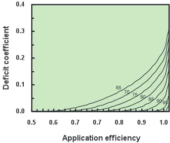
The irrigation application efficiency, thus the irrigation drainage losses, depends on irrigation system factors and management factors. An irrigation system is characterized by its application uniformity. The management factors are considered in the management def-icit coefficient. If the defdef-icit coefficient is high, a large fraction of the field will not receive the water required to maintain full evapotranspiration; on the contrary, if it is low and the application uniformity is low as well, then a significant part of the applied irrigation will be lost as drainage, hence, the application efficiency will be low.
Figure 2.4 depicts the frequency distribution of the applied depth of irrigation (rela-tive to the required depth) across the field assuming that it follows a uniform statistical distribution. Often, the normal distribution adjusts to the non uniformity of the irrigation water better than the uniform distribution. Although the same analysis could be done as-suming a normal distribution (Anyoji and Wu, 1994). Dealing with the uniform distribu-tion is simpler and the unavailability of more precise informadistribu-tion does not justify (in the context of MARSALa) using a more complex model.
figure 2.4 - frequency distribution of the applied depth of irrigation (relative to the re-quired depth) across the field assuming that it follows a cumulated uniform distribution.
For a given required depth, three areas can be distinguished in the graph (see Figure 2.4): area A representing the water that is available for crop consumption, area B represent-ing the water lost by percolation and area C representrepresent-ing the part of the root zone that has not received any irrigation water. Therefore, three irrigation performance indicators may be defined: Application Efficiency (Ea ), Percolation Coefficient (CP) and Deficit Coeffi-cient (CD).
2.3. Irrigation Efficiency Model (Model B)
The irrigation application efficiency, thus the irrigation drainage losses, depends on irrigation system factors and management factors. An irrigation system is characterized by its application uniformity. The management factors are considered in the management deficit coefficient. If the deficit coefficient is high, a large fraction of the field will not receive the water required to maintain full evapotranspiration; on the contrary, if it is low and the application uniformity is low as well, then a significant part of the applied irrigation will be lost as drainage, hence, the application efficiency will be low.
Figure 2.4 depicts the frequency distribution of the applied depth of irrigation (relative to the required depth) across the field assuming that it follows a uniform statistical distribution. Often, the normal distribution adjusts to the non uniformity of the irrigation water better than the uniform distribution. Although the same analysis could be done assuming a normal distribution (Anyoji and Wu, 1994). Dealing with the uniform distribution is simpler and the unavailability of more precise information does not justify (in the context of MARSALa) using a more complex model.
Figure 2.4 - Frequency distribution of the applied depth of irrigation (relative to the required depth) across the field assuming that it follows a cumulated uniform distribution.
For a given required depth, three areas can be distinguished in the graph (see Figure 2.4): area A representing the water that is available for crop consumption, area B representing the water that is lost by percolation and area C representing the part of the root zone that has not received any irrigation water. Therefore, three irrigation performance indicators may be defined: Application Efficiency (Ea), Percolation Coefficient (CP)
and Deficit Coefficient (CD).
(9)
(10)
(9)
2.3. Irrigation Efficiency Model (Model B)
The irrigation application efficiency, thus the irrigation drainage losses, depends on irrigation system factors and management factors. An irrigation system is characterized by its application uniformity. The management factors are considered in the management deficit coefficient. If the deficit coefficient is high, a large fraction of the field will not receive the water required to maintain full evapotranspiration; on the contrary, if it is low and the application uniformity is low as well, then a significant part of the applied irrigation will be lost as drainage, hence, the application efficiency will be low.
Figure 2.4 depicts the frequency distribution of the applied depth of irrigation (relative to the required depth) across the field assuming that it follows a uniform statistical distribution. Often, the normal distribution adjusts to the non uniformity of the irrigation water better than the uniform distribution. Although the same analysis could be done assuming a normal distribution (Anyoji and Wu, 1994). Dealing with the uniform distribution is simpler and the unavailability of more precise information does not justify (in the context of MARSALa) using a more complex model.
Figure 2.4 - Frequency distribution of the applied depth of irrigation (relative to the required depth) across the field assuming that it follows a cumulated uniform distribution.
For a given required depth, three areas can be distinguished in the graph (see Figure 2.4): area A representing the water that is available for crop consumption, area B representing the water that is lost by percolation and area C representing the part of the root zone that has not received any irrigation water. Therefore, three irrigation performance indicators may be defined: Application Efficiency (Ea), Percolation Coefficient (CP)
and Deficit Coefficient (CD).
(9)