Int. J. of Thermodynamics ISSN 1301-9724 Vol. 11 (No. 2), pp. 39-48, June 2008
Axiomatic Definition of Entropy for Nonequilibrium States
Gian Paolo Beretta
Università di Brescia, via Branze 38, 25123 Brescia, Italy
E-mail: [email protected]
Abstract
In introductory courses and textbooks on elementary thermodynamics, entropy is often
presented as a property defined only for equilibrium states, and its axiomatic definition is
almost invariably given in terms of a heat to temperature ratio, the traditional Clausius
definition. Teaching thermodynamics to undergraduate and graduate students from all over
the globe, we have sensed a need for more clarity, unambiguity, generality and logical
consistency in the exposition of thermodynamics, including the general definition of
entropy, than provided by traditional approaches. Continuing the effort pioneered by
Keenan and Hatsopoulos in 1965, we proposed in 1991 a novel axiomatic approach which
eliminates the ambiguities, logical circularities and inconsistencies of the traditional
approach still adopted in many new books. One of the new and important aspects of our
exposition is the simple, non-mathematical axiomatic definition of entropy which naturally
extends the traditional Clausius definition to all states, including non-equilibrium states
(for which temperature is not defined). And it does so without any recourse to statistical
mechanical reasoning. We have successfully presented the foundations of thermodynamics
in undergraduate and graduate courses for the past thirty years. Our approach, including the
definition of entropy for non-equilibrium states, is developed with full proofs in the treatise
E. P. Gyftopoulos and G. P. Beretta, Thermodynamics. Foundations and Applications,
Dover Edition, 2005 (First edition, Macmillan, 1991) [1]. The slight variation we present
here illustrates and emphasizes the essential elements and the minimal logical sequence to
get as quickly as possible to our general axiomatic definition of entropy valid for
non-equilibrium states no matter how “far” from thermodynamic non-equilibrium.
Keywords: second law of thermodynamics, nonequilibrium entropy, definition of entropy,
axiomatic foundations of thermodynamics
1. Introduction
The purpose of this paper is twofold. First, we comment on the motivation by which the “Keenan school of thermodynamics at MIT” (Keenan, Hatsopoulos, Gyftopoulos, Beretta, Zanchini, von Spakovski) has developed a logical sequence of exposition of the axiomatic foundations of thermodynamics in which entropy is defined before heat, and not vice versa as in traditional and most other presentations. Second, we outline and emphasize the important essential hypotheses and the sequence of logical steps of our unconventional order of exposition, which was developed as a means to remove the well-known logical loop which is unavoidable in the traditional definition of entropy based on a heat to temperature ratio, due to the fact that heat and
temperature are almost invariably ill defined by means of some heuristic arguments by which heat is introduced in terms of mechanical illustrations aimed at “demonstrating” the difference between heat and work.
For example, in his lectures on physics that have influenced many generations of physicists, Feynman [2] describes heat as one of several different forms of energy, related to the “jiggling” motion of particles stuck together and tagging along with each other (pp. 1-3 and 4-2), a “form of energy” which really is just kinetic energy— internal motion (p. 4-6), and is measured by random motions of the atoms (p. 10-8). Tisza [3] argues that such slogans as “heat is motion”, in spite of their fuzzy meaning, convey intuitive images of pedagogical and heuristic value.
Int. J. of Thermodynamics, Vol. 11 (No. 2) 40
There are at least three problems with these illustrations. First, work and heat are not stored in a system. Each is a mode of transfer of energy from one system to another. Second, concepts of mechanics are used to justify and make plausible a notion---that of heat---which is beyond the realm of mechanics; although at first the student might find the idea of heat harmless, and even natural, the situation changes drastically when the notion of heat is used to define entropy, and the logical loop is completed when entropy is shown to imply a host of results about energy availability that contrast with mechanics. Third, and perhaps most important, heat is a mode of energy (and entropy) transfer between systems that are very close to thermodynamic equilibrium and, therefore, any definition of entropy based on heat is bound to be valid only at thermodynamic equilibrium.
The first problem is addressed in some expositions. Landau and Lifshitz [4] define heat as the part of an energy change on a body that is not due to work done on it. Guggenheim [5] defines heat as an exchange of energy that differs from work and is determined by a temperature difference. Keenan [6] defines heat as the energy transferred from one system to a second system at lower temperature, by virtue of a temperature difference, when the two are brought into communication. Similar definitions are adopted in widely accepted notable textbooks, such as Van Wylen and Sonntag [7], Wark [8], Huang [9], Modell and Reid [10], Moran and Shapiro [11], and Bejan [12].
None of these definitions, however, addresses the basic problem. The existence of exchanges of energy that differ from work is not granted by mechanics, not even (in our view) after the recent vast physics literature on quantum theories of open systems [13] which has addressed, directly or indirectly, this issue. Indeed, such existence is one of the striking results of thermodynamics, that is, of the existence of entropy as a property of matter. Hatsopoulos and Keenan [14] have pointed out explicitly that without the second law heat and work would be indistinguishable and, therefore, a satisfactory definition of heat is unlikely without a prior statement of the second law.
In our experience, whenever heat is introduced before the first law, and then used in the statement of the second law and in the definition of entropy, the student cannot avoid but sense ambiguity and lack of logical consistency. This results in the wrong but unfortunately widespread conviction that thermodynamics is a confusing, ambiguous, hand-waving, phenomenological subject.
Teaching thermodynamics at MIT to generations of mechanical engineering graduate students from all regions of the globe has evidenced the need for more clarity, unambiguity and logical consistency in the exposition of general thermodynamic principles than provided by traditional approaches. Continuing the effort pioneered at MIT by Keenan [6], Hatsopoulos and Keenan [14], and Hatsopoulos and Gyftopoulos [15,16], Gyftopoulos and the present author [1] have composed an exposition which strives to develop the basic concepts unambiguously and with rigorous logical consistency, building upon the student’s sophomore background in introductory physics and mechanics.
The basic concepts and principles are introduced in a novel sequence that eliminates the problem of incomplete or heuristic definitions, and that is valid for both macroscopic and microscopic well-defined systems, and for both equilibrium and nonequilibrium states. The laws of thermodynamics are presented as general consequences of the fundamental dynamical laws of physics that hold for all well-defined systems. In engineering presentations, like that in Ref. 1, they are presented as laws, rather than theorems of the fundamental dynamical laws, so as to develop a level of description that avoids the full mathematical technicalities required to express such dynamical laws. However, we do not restrict our attention only to the equilibrium domain. Our definition of entropy is more general than that of most textbook where, as Callen [17] stresses, the existence of the entropy is postulated only for equilibrium states and the postulate makes no reference whatsoever to nonequilibrium states.
Heat plays no role in our statement of the first law, in the definition of energy, in our statement of the second law, in the definition of entropy, and in the concepts of energy and entropy exchanges between interacting systems. It is defined using these concepts and laws, after they have been independently and unambiguously introduced. Heat is the energy exchanged between systems that interact under very restrictive conditions that define what we call a heat interaction.
In this paper, we summarize and illustrate the general definition of equilibrium and non-equilibrium entropy first given in Ref. 1. The main reason why we summarize it here and introduce a few minor simplifications and variations with respect to the exposition in Ref. 1, further developed in Ref. 19 and a follow-up forthcoming paper, is to identify and clarify the minimal set of definitions and assumptions which provides the most direct and essential sequence of logical steps
strictly necessary to construct our important and general definition, and present it in an effective way [20].
In view of the importance of non-equilibrium states for a wide range of applications of thermodynamics, we hope our efforts will help to remove statements to the effect that entropy is defined only for equilibrium states from future textbooks.
2. Outline of Our Sequence of Exposition of the Foundations of Thermodynamics (Up to the Definition of Entropy)
Here we outline schematically the logical sequence of exposition that we adopt in our book [1], to which the reader is referred for full details and proofs. In an undergraduate course focused on engineering applications, in class we skip most proofs (interested students can find them in the book) and in about six to eight 45-min lectures we develop the foundations of the subject according to the following sequence.
2.1 Basic definitions, first law, energy and energy balance
We define the scope of thermodynamics as that of describing the properties of physical systems and how they evolve in time. We define what we mean by the term “system” (a ‘separable’ set of elementary constituents subject to internal forces, internal partitions and external forces which may depend on parameters but not on coordinates of external objects; examples show that ‘non-separable’ objects do not qualify as well-defined systems). We define what we mean by the terms “amounts of constituents” (result of a counting measurement procedure characterizing the system’s preparation at one instant of time), “property” (repeatable measurement procedures characterizing the system’s preparation by yielding a numerical result that depends only on one instant of time) and “state” (list of values at one instant of time of all the amounts, n, of constituents, all the parameters, ββββ, of the external forces, and all the conceivable properties of the system).
We explain that a full description of how the state of the system evolves in time requires the consideration and solution of its general equation of motion. Instead of taking this approach, which is postponed to more advanced and theoretical treatments, we focus on the two most general theorems of the equation of motion that are universal features of the dynamics of any (well-defined) system. Such theorems are captured by the two general non-mathematical statements valid for all systems that we call the first law and the second law. We call them “laws” or “principles”
because in our exposition they are not proved from the analysis of the equation of motion, but are adopted and postulated as the dynamical features that cannot be violated by any evolution of any well-defined system. To move towards the statements of these two laws, we introduce the concepts of “process” (initial and final states of a system; description of the effects left in its environment, i.e., in principle the rest of the universe), “spontaneous change of state”, “isolated system”, and “weight process” (the only external effect is the change in height of a weight).
We then state the first law (every pair of states of any given system can be interconnected by means of a weight process) and prove that it entails the existence of a property, that we call “energy”, whose differences are defined by a measurement procedure by which we interconnect the given state and an arbitrary reference state (selected once and for all for the system) by means of a weight process and measure the change in potential energy of the weight (the potential energy of a simple weight is a concept assumed known from previous courses in mechanics). We emphasize that the virtue of the first law is to extend the concept of energy from the domain of mechanics to the broader domain of thermodynamics. We then show that energy is an “additive” property, it is “conserved” (remains constant in spontaneous changes of state, i.e. for isolated systems), and it can be “exchanged” between interacting systems; we denote by E12← the net energy exchanged during the time interval t1-t2 (positive if received by the system). Hence,
we introduce the energy balance equation
←
= − 1 12
2 E E
E .
2.2 Second law and other basic definitions To introduce the second law, we then classify states in terms of their time dependence (steady, unsteady, equilibrium and non-equilibrium), further classifying equilibrium states in terms of their stability (unstable, metastable and stable). A “stable equilibrium state” is one that cannot be altered without leaving net effects in the environment of the system (as shown in Ref. 18, this is a non-mathematical expression of the technical definition of stability for a dynamical system according to Lyapunov).
The second law is introduced as the answer to the question: “How many stable equilibrium states does a system admit?”, a question that clearly addresses a fundamental feature of the dynamics. The answer is the Hatsopoulos-Keenan statement of the second law (among all the states of a system that have a given set of values of the
Int. J. of Thermodynamics, Vol. 11 (No. 2) 42
energy, the amounts of constituents, and the parameters of the external forces and the internal partitions, one and only one is a stable equilibrium state). We “promise” that by adopting this statement of the second law, in due course we will prove that every other traditional statement that the student might have seen in his previous career (Clausius, Kelvin-Planck, Carathèodory) follows as a theorem.
To proceed we need to introduce three new concepts: the definitions of “mutual stable equilibrium,” of “thermal reservoir,” and of “reversible process.”
Two systems, A and B, are in “mutual (stable) equilibrium” if the composite AB of the two systems is in a stable equilibrium state.
A “thermal reservoir” or simply a “reservoir” is any system with a set of stable equilibrium states that differ in energy1 but are all in mutual stable equilibrium with a given system in a given fixed stable equilibrium state.2
A “reversible process” is a process for which another process exists that takes the system back to its initial state while also all the external effects are undone. In particular, a “reversible weight process” is a weight process for which another weight process exists that takes the system back to its initial state while also the change in height of the weight, which is the only external effect of the weight process, is undone.
A further part of our second law statement, is that any state of any system can be interconnected to some stable equilibrium state by means of a reversible weight process.
We now have enough concepts to define three important properties characterizing each thermal reservoir R with respect to a reference thermal reservoir R0 (such as, to fix ideas, that
obtained with water at the triple point3).
To define them, we consider an arbitrary auxiliary system A, an arbitrary pair A1 and A2 of
its states, and a reversible “standard” weight process for the composite system AR in which system A changes from state A1 to state A2 (by
1
At this stage of the development it suffices to introduce a thermal reservoir with fixed parameters ββββ (such as for example the volume V) and fixed amounts of constituents n, so that, by the statement of the Second Law, its stable equilibrium states differ only by the value of the energy. Later on, this notion is generalized to reservoirs with variable parameters and/or variable amounts of constituents.
2
Any pure substance in a ‘triple point’ set of states is an example of reservoir. Water at the triple point is relatively easily reproducible in every laboratory and is therefore taken as a ‘reference’ reservoir.
“standard” we mean that the initial and final states of the reservoir are stable equilibrium states [20]).
In this process we are interested in the change in energy of the reservoir R, that we denote3 by
rev sW,
2 1
)
(∆ER AA , and compare it with the change
rev sW,
2 1 0)
(∆ER AA that obtains when (for the same states A1 and A2 of system A) we consider a
reversible “standard” weight process for the composite system AR0.
2.3 Definition of temperature of a thermal reservoir
When states A1 and A2 are chosen so that
they (a) have the same values of all parameters ββββ, (b) have the same values of all amounts n of constituents, and (c) cannot be interconnected by means of a reversible weight process for system A, the ratio n A A R n A A R E E , rev sW, , rev sW, 2 1 0 2 1 ( ) ) ( β β ∆ ∆ can
be proved [1, par.7.4, p. 108] to be positive and independent of (i) the specific choice of states A1
and A2, (ii) the specific choice of system A, (iii)
the initial (stable equilibrium) state of reservoir R, and (iv) the initial (stable equilibrium) state of reservoir R0; therefore, it depends only on the pair
of reservoirs, R and R0, regardless of their states.
Even if we do not present this proof in an introductory course, the fact that it is available in Ref. 1, in our experience gives the student sufficient confidence to trust that we are proceeding rigorously on logically consistent grounds.
Based on this result, with respect to the reference reservoir R0, for the stable equilibrium
states of a reservoir R we define the property
0 , rev sW, 2 1 0 rev sW, 2 1 ) ( ) ( R n A A R A A R R T E E T β ∆ ∆ =
which we call4 “absolute temperature of the thermal reservoir” and has the same value for all the stable equilibrium states of R. By selecting water at the triple point as the reference reservoir R0 and choosing 273.16K
0 = R
T , defines the
“Kelvin scale” for T . R
3
For completeness, in this paper we adopt a more cumbersome notation than in Ref. 1. The purpose is to make explicit in each symbol all the many important hypotheses of the subsequent definitions. In class, we sometimes adopt a lighter notation.
4
Warning: this is not yet the definition of temperature for a system which is not a reservoir!
At this stage of the development, in an introductory course, it suffices to consider systems and thermal reservoirs with fixed parameters ββββ (such as for example the volume V) and fixed amounts of constituents n, leaving for a later stage the generalization to systems and reservoirs with variable parameters and/or variable amounts of constituents. Thus, in the interest of simplicity, we may jump to Section 2.6 and conveniently postpone the next two sections where, for completeness, we define two more properties of a thermal reservoir.
2.4 Definition of total potentials of a thermal reservoir
When states A1 and A2 are chosen so that
they (a) have the same values of all parameters ββββ, and (b) have the same values of all amounts n of constituents except for that of one constituent, ni,
the difference ' , rev sW, 0 0 ' , rev sW, 2 1 0 2 1
1
1
n A A iR R R n A A iR R Rn
E
T
n
E
T
β β
∆
∆
−
∆
∆
can be proved to be independent of (i) the specific choice of states A1 and A2, (ii) the specific choice
of system A, (iii) the initial (stable equilibrium) state of reservoir R, and (iv) the initial (stable equilibrium) state of reservoir R0; therefore, it
depends only on the pair of reservoirs, R and R0,
regardless of their states. Based on this result, with respect to the reference reservoir R0, for the stable
equilibrium states of a reservoir R we define the property + ∆ ∆ = ' , rev sW, 2 1A n A iR R iR n E β µ ∆ ∆ − + ' , rev sW, 0 0 2 1 0 0 n A A iR R iR R R n E T T β µ
which we call5 “total potential of component i of the thermal reservoir”. It has the same value for all the stable equilibrium states of R. By selecting arbitrarily the value of
0 iR
µ for a reference reservoir R0 consisting, for example, of each pure
“elemental” substance i at its solid-liquid-vapor triple point, we obtain one possible6 absolute scale
5
This is not yet the definition of total or chemical potential for a system which is not a reservoir.
6
Elemental species are defined e.g. in Ref. 1 at page 545. Since any other species can be obtained from the
for iR
µ . Here, subscript n' means that all amounts n except ni are kept constant; superscript
sW,rev still means that the composite system AR undergoes a “reversible standard weight process” for which it must be clear that since the only external effect is the change in height of a weight, there is no change in parameters of either A or R, nor change in the overall amounts of constituents of AR, although in the process, A and R exchange the amount 0 1 2 iR iR R A i A i A i n n n n n − = ← =−∆ =−∆ of constituent i.
2.5 Definition of pressure of a thermal reservoir
When states A1 and A2 are chosen so that
they (a) have the same values of all parameters ββββ except for the volume, V, and (b) have the same values of all amounts n of constituents, the difference n A A R R n A A R R R VR E T V E T ,' rev sW, 0 0 ,' rev sW, 2 1 0 2 1 1 1 β β ∆ ∆ − ∆ ∆
can be proved to be independent of (i) the specific choice of states A1 and A2, (ii) the specific choice
of system A, (iii) the initial (stable equilibrium) state of reservoir R, and (iv) the initial (stable equilibrium) state of reservoir R0; therefore, it
depends only on the pair of reservoirs, R and R0,
regardless of their states. Based on this result, with respect to the reference reservoir R0, for the stable
equilibrium states of a reservoir R we define the property + ∆ ∆ − = n A A R R R V E p ,' rev sW, 2 1 β ∆ ∆ + + n A A R R R R R V E p T T ,' rev sW, 0 0 2 1 0 0 β
which we call7 “pressure of the thermal reservoir”. It has the same value for all the stable equilibrium states of R. Because later on in the treatment it is shown that it is equal to the force per unit area that the constituents exert on the walls of the reservoir, selecting water at the triple point as the reference reservoir R0 and choosing pR0 =0.611kPa,
yields the absolute pressure scale.
elemental set via a chemical reaction of formation, the reference value µiR0 is conveniently selected equal to the molar Gibbs free energy of formation [1, p.547].
7
This is not yet the definition of pressure for a system which is not a reservoir.
Int. J. of Thermodynamics, Vol. 11 (No. 2) 44
Here, subscript β' means that all parameters
ββββ except the volume V are kept constant. Superscript sW,rev means again that the composite system AR undergoes a “reversible standard weight process” for which it is clear that since the only external effect is the change in height of a weight, here there is no change in the amounts of constituents nor in any parameters other than the volumes of A and R. Of course, the overall volume of AR does not change, while A and R ‘exchange’ the volume V2A−V1A=VA←R =−∆VR =−∆VR0.
2.6 Definition of entropy
We have now built enough concepts to proceed to our definition of entropy valid for all states. However, depending on our teaching goals, we may choose to proceed along two different but equivalent paths.
The first, which we propose in Ref. 1, gets to the definition of entropy through the definition of the intuitive and empirically important properties that we call “adiabatic availability” and “available energy with respect to a thermal reservoir”.
The second, which we developed later and is outlined for example in Ref. 19, goes directly to the definition of entropy. It is a more direct and essential path, but being more abstract it is sligthly less intuitive.
Below, we present both paths: the first in Section 2.7a, the second in Section 2.7b.
2.7a Path 1: “Availability first”
We address the fundamental question: “How much energy can we extract from a system A by means of a weight process?”. The answer is in the theorem of existence of a property, that we call “adiabatic availability”, defined by the raise in potential energy of the weight in a measurement procedure by which we interconnect the given state A1 with the only stable equilibrium state, AS1,
that can be reached by means of a reversible weight process (at fixed amounts of constituents and fixed parameters). That this defines a property for any state A1 of system A, including
non-equilibrium states, is a consequence of the first law and the second law together; we usually do not present in class the full proof, but just mention that it is given in Ref. 1. We denote the value of the adiabatic availability of state A1 by Ψ . 1
We show that energy and adiabatic availability can be used to ascertain whether a given weight process for system A, say from state A1 to state A2, is reversible, irreversible or
impossible: we must evaluate E and 1 Ψ for state 1
A1, E and 2 Ψ for state A2 2, and then verify
whether the difference (E2−Ψ2)−(E1−Ψ1) is zero, positive or negative, respectively. From this result we see that the difference E−Ψ (“adiabatic unavailability”) has some of the important features of entropy (it satisfies a principle of non-decrease in any weight process), but it has the drawback of not being additive. This observation motivates the subsequent effort to construct the definition of a new property (entropy) monotonically related to
Ψ −
E , but additive.
We now address again the previous question but for a more specific situation of very practical interest: “How much energy can we extract from a system C by means of a weight process when system C is composed of a system A and a thermal reservoir R?” By the results just derived, the answer is of course that the largest amount that can be extracted is the adiabatic availability of system C, and is therefore a property of the combination system-reservoir. This property is empirically very important because the “natural environment,” in which we live and develop our machineries and energy conversion systems, is very well approximated by a thermal reservoir.
Because of the special defining features of a reservoir, the adiabatic availability of a composite AR turns out to be independent of the initial state of the reservoir, therefore, for a fixed R, it depends only on the state of system A, i.e., it is a property of system A only. Thus, when viewed as a property of system A with respect to a given reservoir R. If system A has fixed values of n and
ββββ we call this property “available energy with respect to reservoir R” and for state A1 we denote
it by the symbol Ω1R (which of course is equal to the adiabatic availability Ψ11AR of AR in state A1R1). In a broad sense this property is an
“availability” or “exergy” function.8
More generally, if system A has variable values of n and ββββ,,,, we call this property “generalized available energy with respect to reservoir R” and here we adopt the symbol Ξ1R.
The important advantage of this new property is that it is additive, and it preserves some of the key features of adiabatica availability. In particular, we show that it too can be used to ascertain whether a given weight process for system A, say from state A1 to state A2, is
reversible, irreversible or impossible: we must evaluate E1 and Ω1R for state A1, E2 and ΩR2 for
8
More generally, if system A has variable values of n and V, and fixed all other ββββ’s we call this property “generalized available energy with respect to reservoir R” and here we adopt the symbol Ξ1R.
state A2, and then verify whether the difference
) (
)
(E2−Ω2R − E1−Ω1R is zero, positive or negative, respectively. From this result we see that the difference E−ΩR (“unavailable energy” with respect to reservoir R) has some of the important features of entropy (it satisfies a principle of non-decrease in any weight process), and it is additive, but it has the drawback of depending on the reservoir R. This observation motivates the subsequent and final step to preserve the two features but construct a property of system A only.
Therefore, we finally define the property “entropy” whose difference for two states of a system A with fixed values of n and ββββ is given by
R R R T E E S S2− 1=( 2−Ω2)−( 1−Ω1)
Indeed, by a simple energy balance we show that in general ) ( ) ( ) ( 1 1 2 2 , rev sW, 2 1 R R n A A R E E E = −Ω − −Ω ∆ β
and, using our important result in Section 2.3, we show that 0 2 1 0 2 1 , rev sW, , rev sW, 1 2
)
(
)
(
RT
E
T
E
S
S
R AA n R n A A R β∆
β−
=
∆
−
=
−
and hence it is independent of R. This proves that the reservoir R plays only an auxiliary role in our definition of entropy differences. Because no restriction has been necessary on either the system A or its states, this definition holds valid for all systems and all states.9
9
More generally, for a system A with variable values of n and V, and fixed all other ββββ’s, entropy differences are defined by + Ξ − − Ξ − = − R R R T E E S S2 1 ( 2 2) ( 1 1)
∑
− − − + i R i i iR R R T n n T V V p ( 2 1) µ ( 2 1)Also here, by an energy balance we note that
) ( ) ( ) ( 1 1 2 2 ' rev sW, 2 1 R R A A R E E E = −Ξ − −Ξ ∆ β
and to prove that the difference S −2 S1 is independent of the choice of the reservoir R it suffices to use the results of Sections 2.4 and 2.5, and split the change between states A1 and A2 into a sequence of steps
We finally prove that entropy differences are additive, and that entropy satisfies a theorem of non-decrease in weight processes, and can be exchanged between interacting systems. We denote by S12← the net energy exchanged during the time interval t1-t2 (positive if received by the
system). Hence, we introduce the entropy balance inequality S2−S1≥S12← or, equivalently and more conveniently, the entropy balance equation
gen 12 1
2 S S S
S − = ←+ , where of course Sgen ≥0
represents the entropy generated in the system if the process is irreversible.
We then prove the “maximum entropy theorem” (or “principle”) which states that every state which is not stable equilibrium has entropy strictly lower than the entropy of the stable equilibrium state with the same values of E, n and
ββββ . We also prove the “state principle” and the existence of the “fundamental relation for the stable equilibrium states”, S =S(E,V,n,β') and its inverse E =E(S,V,n,β'). From these theorems we derive the necessary conditions for mutual stable equilibrium between systems, which motivate and prompt us to give the general definitions of “temperature”, “pressure”, “total potentials” for stable equilibrium states of any system (not just a reservoir) in terms of the partial derivatives of the fundamental relation in energy form, respectively, T =∂E(S,β,n)/∂S, V n V S E p=−∂ ( , , ,β')/∂ ,µi =∂E(S,β,n)/∂ni. 2.7b Path 2: “Entropy first”
We define immediately the measurement procedure that defines the new property entropy. To measure the entropy difference between any two given states A1 and A2 of a system A, we
select arbitrarily an auxiliary reservoir R and consider a reversible “standard” weight process for the composite system AR. For the change in energy of the reservoir R in this process we have introduced the notation sW,rev
2 1 ) (∆ER AA .
If states A1 and A2 have the same values of n
and ββββ we define R n A A R T E S S , rev sW, 1 2 2 1 ) ( β ∆ − = −
and, as shown in Section 2.7a, we use the result of Section 2.3 to show that the ratio on the r.h.s. is invariant upon change of reservoir R with
whereby the volume and each amount constituents change one at a time.
Int. J. of Thermodynamics, Vol. 11 (No. 2) 46
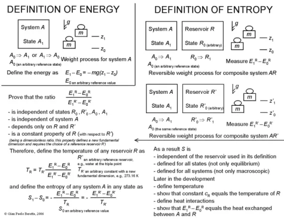
any other reservoir.10 Figure 1. summarizes this approach in a single sketchy viewgraph.
We next state that entropy differences are additive, that entropy satisfies a theorem of non-decrease in weight processes, and that it can be exchanged between interacting systems. Thus, as at the end of Section 2.7a we introduce: the “entropy balance equation”, the “maximum entropy theorem”, the “fundamental relation for the stable equilibrium states”, the necessary conditions for mutual stable equilibrium between systems, and the general definitions of “temperature”, “pressure”, and “total potentials” as the partial derivatives of the fundamental relation in energy form (defined for stable equilibriun states only).
With this we can move on to the questions that define adiabatic availability and available energy with respect to a reservoir and derive their expressions in terms of energy and entropy, by means of energy and entropy balances. These derivations can be also done graphically with the help of our energy versus entropy graphs [1, Ch. 14] which constitute a very effective teaching tool, that helps to fix and summarize all the basic results, and to reason in a logically consistent way.11
In particular, we derive the following practical relations. For the adiabatic availability of state A1
1 1 1=E −ES Ψ
where state AS1 is defined by the condition
1
1 S
SS = . For the available energy with respect to reservoir R of state A1 of a system A with fixed n
and ββββ ) ( 1 1 1R =E −ER−TR S −SR Ω
where ER and SR denote the energy and the entropy
of system A in the state AR of mutual stable
equilibrium with the reservoir, i.e., at temperature
10
If states A1 and A2 have the different values of n
and V, whereas all other ββββ’s are fixed, we define
R A A i iR iR R R R T n V p E S S ' rev sW, 1 2 2 1 ) ( β µ
∑
∆ − ∆ + ∆ − = −where of course ∆VR =V1A−V2A and
A i A i iR n n n = 1− 2
∆ because by definition of weight process the volume and the amounts of the overall system AR must not change.
11 For example it helps very much in visualizing the
reasoning underlying the delicate definition of “heat interaction” [20].
TR and the given fixed values of n and ββββ. For the
generalized available energy with respect to reservoir R of state A1 of a system A with variable
n and V, and fixed all other ββββ’s
+ − − − = Ξ1R E1 ER TR(S1 SR) ) ( ) ( 1 R i iR i1 iR R V V n n p − − − +
∑
µwhere again ER, SR , VR, and niR denote the energy,
the entropy, the volume and the amounts of constituents of system A in the state AR of mutual
stable equilibrium with the reservoir, i.e., at temperature TR, pressure pR, total potentials µiR’s,
and the given fixed values of the other ββββ’s. 3. Conclusions
We have outlined and illustrated the essential elements and the minimal logical sequence we developed to introduce in rigorous terms a general axiomatic definition of entropy valid for non-equilibrium states no matter how “far” from thermodynamic equilibrium.
It is important to note that up to the definition of entropy, our logical development does not make use of the “fundamental relation for the stable equilibrium states”, nor of the definitions of “temperature”, “pressure”, “total potentials” for such states, which are given later in terms of its partial derivatives.
Moreover, it is only later in the development that we define “work interactions” as those in which no entropy is exchanged, and “heat interactions” as those in which energy and entropy are exchanged between two systems that initially are both in stable equilibrium states at nearly the same temperature.
Still much later, by introducing what we call “the simple system model” we specialize the treatment to systems with a sufficiently high number of particles so that wall-rarefaction effects are negligible. For these systems, we show that the fundamental relation S =S(E,V,n,β') for the stable equilibrium states is homogeneous of the first degree in E, V, n, and all other additive parameters [1,Ch.17], so that we gain the Euler relation and many well-known standard results. But we emphasize that the wealth of results we derive in Ref. 1 before introducing the simple system model hold for all systems, including micro, nano and few-particle systems, that have today become within reach of experiments and practical applications.
Nomenclature Symbols
A without subscript denotes a system, with subscript denotes a state
E energy S entropy V volume T temperature t time p pressure n amount of constituent
n = {n1, n2, …, nr} amounts of all constituents
β parameters of the Hamiltonian, e.g., of the external forces (geometry of container, volume, etc)
Ψ adiabatic availability
ΩR available energy with respect to a reservoir R with fixed amounts and parameters
Ξ generalized available energy with respect to a reservoir R with variable amounts and parameters
µ total potential
∆ difference between final and initial value Subscripts
0 reference
1 state 1; instant of time 1 2 state 2; instant of time 2
R belonging to reservoir R; referred to a system identifies the state R in which the system is in mutual equilibrium with reservoir R i belonging to constituent i
n fixed values of all the constituents n’ fixed values of all other constituents β fixed values of all parameters β’ fixed values of all other parameters gen generated by irreversibility
12 in a process occurred between times t1 and t2;
or in a process in which the system changes between states 1 and 2
Superscripts
sW standard weight process rev reversible process
← exchanged by the system via interaction (positive if into the system)
→ exchanged by the system via interaction (positive if out of the system)
References
[1] E. P. Gyftopoulos and G. P. Beretta, Thermodynamics. Foundations and Applications, Dover, Mineola, 2005 (First edition, Macmillan, 1991).
[2] R. P. Feynman, Lectures on Physics, Vol. 1, Addison-Welsey, 1963.
[3] L. Tisza, Generalized Thermodynamics, MIT Press, 1966, p. 16.
[4] L. D. Landau and E. M. Lifshitz, Statistical Physics, Part I, 3rd Ed., Revised by E. M. Lifshitz and L. P. Pitaevskii, Translated by J. B. Sykes and M. J. Kearsley, Pergamon Press, 1980, p. 45.
[5] E. A. Guggenheim, Thermodynamics, North-Holland, 7th Ed., 1967, p. 10.
[6] J. H. Keenan, Thermodynamics, Wiley, 1941, p. 6.
[7] G. J. Van Wylen and R. E. Sonntag, Fundamentals of Classical Thermodynamics, Wiley, 2nd Ed., 1978, p. 76.
[8] K. Wark, Thermodynamics, 4th Ed., McGraw-Hill, 1983, p. 43.
[9] F. F. Huang, Engineering Thermodynamics, Macmillan, 1976, p. 47.
[10] M. Modell and R. C. Reid, Thermodynamics and Its Applications, Prentice-Hall, 1983, p. 29.
[11] M. J. Moran and H. N. Shapiro, Fundamentals of Engineering Thermodynamics, Wiley, 1988, p. 46.
[12] A. Bejan, Advanced Engineering Thermo-dynamics, 2nd Ed., Wiley, 1997.
[13] H. P. Breuer and F. Petruccione, The Theory of Open Quantum Systems, Oxford University Press, 2002.
[14] G. N. Hatsopoulos and J. H. Keenan, Principles of General Thermodynamics, Wiley, 1965, p.xxiii.
[15] G. N. Hatsopoulos and E. P. Gyftopoulos, Foundations of Physics, Vol. 6, 15, 127, 439, 561 (1976).
[16] G. N. Hatsopoulos and E. P. Gyftopoulos, Thermionic Energy Conversion, Vol. II, MIT Press, 1979.
[17] H. B. Callen, Thermodynamics, and an Introduction to Thermostatics, 2nd Ed., Wiley, 1985.
[18] G. P. Beretta, Journal of Mathematical Physics, Vol. 27, 305 (1986).
[19] E. Zanchini and G. P. Beretta, in Meeting the Entropy Challenge, Ed. G. P. Beretta, A. Ghoniem, and G. N. Hatsopoulos, AIP Proceedings Series, in press (2008).
[20] An example of a 90 min lecture by the author titled “Thermodynamics in a nutshell – The definition of entropy in one lecture” can be viewed at the permanent MIT-TechTV on-line archive http://techtv.mit.edu/file/607 (January, 2008).
Int. J. of Thermodynamics, Vol. 11 (No. 2) 48
Figure 1. Schematic ‘blackboard summary’ of the essential conceptual steps of the axiomatic definition of entropy introduced in Ref. 1 (where full details and proofs can be found in Chapters 5 to 7).