Testing for Parameter Stability in Dynamic
Models across Frequencies
∗
Bertrand Candelon
University of Maastricht
Gianluca Cubadda
Università di Roma "Tor Vergata"
September 20, 2005
Abstract
This paper contributes to the econometric literature on structural breaks by proposing a test for parameter stability in VAR models at a particular frequency ω, where ω ∈ [0, π]. When a dynamic model is affected by a structural break, the new tests allow for detecting which frequencies of the data are responsible for parameter instability. If the model is locally stable at the frequencies of interest, the whole sample size can be then exploited despite the presence of a break. Two empirical examples illustrate that local instability can concern only the lower frequencies (decrease in the postwar U.S. productivity) or higher frequencies (change in the U.S. monetary policy in the early 80’s).
Keywords: Structural breaks, spectral analysis, productivity slowdown, yield curve. JEL: C32, E43
∗We are grateful to Marco Centoni for discussions and comments on the paper, as well as to the participants
of the ESF-EMM 2004 meeting in Alghero, the First Italian Congress of Econometrics and Empirical Economics in Venice, the Frontier in Time Series Congress in Olbia, and the First meeting of the Netherlands Econometric Study Group in Amsterdam. Gianluca Cubadda gratefully acknowledges financial support from MIUR.
1
Introduction
Tests for structural changes are important tools in the statistical analysis of economic time series. In this respect, the well-known Chow (1960) test still constitutes a standard reference. It consists of splitting the sample into two sub-periods, before and after the break, and testing the equality of the parameters between the two sub-samples, using an asymptotic χ2 distri-bution. Because of its simplicity of implementation, it is still used in many empirical studies. Nonetheless, this test was extended in several directions.1
Firstly, instead of considering the date of the break as known, the testing procedure should treat it as a unknown parameter to be estimated. Following the seminal paper of Quandt (1960), a recursive sequence of Chow tests is performed, dating the break at the point where the test statistic takes the largest value. Andrews (1993) delivers the most important contribution for this extension by defining the asymptotic distribution of the sup-Chow test, which is no longer a χ2 distribution. A further extension in this direction is developed by Bai and Perron (1998, 2003), who consider the case of multiple structural breaks with unknown dates. These authors propose several iterative methods to test for the number of breaks, and derive the asymptotic distributions of the relevant test statistics. All these procedures are valid for single equation models with no trending regressors, such as deterministic trends or I(1) processes.
The above approaches have recently been extended to multivariate regression models. Bai et al. (1998) generalized the single break framework in Andrews (1993) to multiple time series that are either stationary or cointegrated in the regimes of parameter stability. They showed that statistical inference is more precise when series having a common break are jointly analyzed. Bai (2000) considered the issue of multiple breaks in a segmented stationary VAR model and proved that the number of change points can be consistently estimated via information criteria, whereas Qu and Perron (2004) proposed a quasi maximum likelihood approach to analyze multiple breaks in multivariate regression models.
Secondly, some papers were devoted to the application of the standard Chow test to the Vector Error Correction Model (VECM). Hansen (2003), inter alia, provided tests for a break in the coefficients of the VECM, though his results are restricted to the case of known break dates. In particular, a partial structural change can be present in the cointegration parameters or in the adjustment coefficients. Such an extension has interesting economic implications, as it is possible to interpret a structural break as affecting the long-run (partial change in the cointegration relationships) or the short-run (partial change in the adjustment coefficients).
The present paper generalizes the previous idea by proposing a test for parameter stability in a segmented stationary or cointegrated VAR model at a particular frequency ω, where ω ∈ [0, π]. Hence, if a VAR model is affected by a structural break, it is then possible to detect which frequencies of the data are responsible for parameter instability. Moreover, if a researcher wishes to concentrate on a subset of the frequencies of the data, the proposed test allows one to check
wether the whole sample size can be exploited for the analysis, despite the presence of a break. Although the null hypothesis of local stability at frequency ω implies that the spectral density matrix at frequency ω is stable over time, the testing procedure is easily implemented in the time domain,2 as it is based on a set of linear hypotheses on the autoregressive parameters. The test statistic for local stability at a given frequency has a limit χ2 distribution when the break date is either known or estimated by means of the sup-Chow test for a full structural change. For the latter case, a bootstrap procedure is also offered. We evaluate the finite-sample behavior of our testing procedure through a Monte Carlo study.
The test procedure is applied to two well known examples. The first one copes with the slowdown of the post-war United States output growth. Following King et al. (1991), we consider a trivariate system with consumption, investment and output to get a clearer view on this issue. Similarly to Bai et al. (1998), a structural break is detected in the late sixties, and our local stability tests reveal that the system is unstable only at low frequencies. This evidence is consistent with the view that a negative productivity shock is at the origin of the break.
The second example concerns the predictive power of the yield curve on future output growth in the U.S. It turns out that a break is detected around July of 1980. Based on Estrella et al. (2003), we interpret this break as the consequence of a change in monetary policy associated with the nomination of Paul Volcker as the head of the FED. Our local stability tests confirm this hypothesis by stressing that the relationship between the spread and future output growth remains stable at low frequencies. Local instability is nevertheless found at business and seasonal frequencies.
The paper is organized as follows. In section 2, the concept of local stability at frequency ω is developed for segmented stationary VAR systems and known break dates. The extensions for cointegrated systems and unknown break dates are proposed in Section 3. In section 4, a simulation study is performed to investigate the properties of the tests. Section 5 presents both the empirical applications, and Section 6 concludes.
2
Local stability in stationary VAR models
Let us consider a n-vector time series {Xt, t = 1, . . . , T } that is generated by the following
stationary linear stochastic process
Xt= ΘDt+ C(L)εt, (1)
where C(L) = In+P∞i=1CiLi is such that P∞j=1j |Cj| < ∞, εt are i.i.d. Nn(0, Σ)
innova-tions, and Dt is a m-vector of deterministic terms that may contain a constant and various
trigonometric functions of time.
2
Similar approaches can be found in Breitung and Candelon (2005) for Granger-causality tests, Centoni and Cubadda (2003) for measuring the cyclical effects of permanent-transitory shocks, and Christiano and Vigfusson (2003) for maximum likelihood analysis of business cycle models.
We assume that series Xt admits the following VAR(p) representation:
A(L)Xt= ΦDt+ εt, t = 1, . . . , T, (2)
where A(L) = In−Ppi=1AiLi is such that det [A(c)] = 0 implies that |c| > 1, and ΦDt =
A(L)ΘDt.
By expanding the polynomial matrix A(L) on 0 and the complex conjugate points z and z−1, where z = exp(−iω) and ω ∈ [0, π], we rewrite equation (2) as follows:
∆ω(L)Xt= ΦDt+ Πω(L)Xt−1+ Γω(L)∆ω(L)Xt−1+ εt, (3) where ∆ω(L) = ( 1 − 2 cos(ω)L + L2 if ω ∈ (0, π) (1 − zL) if ω = 0 or ω = π , Πω(L) = (
− Im[A(z)]/ sin(ω) + (Re[A(z)] + cot(ω) Im[A(z)])L if ω ∈ (0, π)
−zA(z) if ω = 0 or ω = π , and Γω(L) is a n × n polynomial matrix of order (p − 3) if ω ∈ (0, π), (p − 2) if ω = 0 or ω = π.3
Since the filter ∆ω(L) annihilates at L = z, the filtered series ∆ω(L)(Xt− ΘDt) have null
spectra at frequency ω. Hence the parameters Πω(L) fully characterize the stochastic behavior
of series Xt at frequency ω. Indeed, the spectral density matrix of the stochastic process
(Xt− ΘDt) at frequency ω is given by C(z)ΣC(z−1)0, where C(z) = Πω(z)−1.
The frequency domain properties of model (2) are also determined by the nature of the deter-ministic vector Dt. Indeed, a linear combination of the trigonometric functions [cos(ωt), sin(ωt)]
has its spectral mass entirely concentrated at frequency ω. Hence, let us write ΦDt= Φ1D1,t+ Φ2D2,t,
where D1,t and D2,t are respectively composed of m1 and m2 elements such that
∆ω(L)D1,t= 0,
∆ω(L)D2,t6= 0.
It is clear that the parameters Φ1 fully characterize the deterministic behavior of series Xt at
frequency ω.
We now allow for a possible structural break at time Tb = bT , where b ∈ (0, 1). Let us
assume, for the moment, that there is only one single break and its date Tb is known. Model
3
(2) is then generalized by the following sub-sample models: A−(L)Xt = Φ−Dt+ εt, t = 1, . . . , Tb, (4) A+(L)Xt = Φ+Dt+ εt, t = Tb+ 1, . . . , T, (5) where A−(L) = In−Pp i=1A−i Li, A+(L) = In− Pp i=1A +
i Li, and the roots of both det [A−(L)] and
det [A+(L)] lie outside the unit circle.
Notice that we can expand both the polynomial matrices A−(L) and A+(L) on 0 and the complex conjugate points z and z−1, thus obtaining the sub-sample analogs of model (3). Hence, let us consider the following particular cases of the sub-sample models (4) and (5):
∆ω(L)Xt = Φ1D1,t+ Φ−2D2,t+ Πω(L)Xt−1+ Γ−ω(L)∆ω(L)Xt−1+ εt, (6)
t = 1, . . . , Tb,
∆ω(L)Xt = Φ1D1,t+ Φ+2D2,t+ Πω(L)Xt−1+ Γ+ω(L)∆ω(L)Xt−1+ εt, (7)
t = Tb+ 1, . . . , T,
where Γ−
ω(L) and Γ+ω(L) are n × n polynomial matrices of orders (p − 3) if ω ∈ (0, π), (p − 2) if
ω = 0 or ω = π.
Since the structural break does not affect the components of series Xt that are associated
with fluctuations at frequency ω, the sub-sample models (6) and (7) are said to be locally stable at that frequency. Notice that local stability is possible only if the polynomial parameter matrices Γ−ω(L) and Γ+(L) can freely vary from Πω(L). Therefore, a necessary condition for
local stability at frequency ω is that p > 2 if ω ∈ (0, π) and p > 1 if ω = 0 or ω = π. The statistical problem consists of testing for each of the following null hypotheses:
H0 (global stability): [A−(L) = A+(L)] ∩ [Φ−= Φ+],
H∗ (local stability): [Γ−
ω(L) 6= Γ+ω(L)] ∩ [Φ−2 6= Φ+2],
versus the alternative hypothesis:
H1 (global instability): [A−(L) 6= A+(L)] ∩ [Φ−6= Φ+].
In particular, the sample-split Chow test statistics (see e.g. Doornik and Hendry, 1997) for the systems of hypotheses H0 versus H1 and H∗ versus H1 are, respectively, the following:
Ξ0|1(b) = (T − 2p − q0) det à T P t=p+1bε 0 tbεt ! − det à TPb−1 t=p+1bε −0 t bε−t + T P t=Tb bε+0t bε + t ! det à TPb−1 t=p+1bε −0 t bε−t + T P t=Tb bε+0t bε+t ! → κd 2(q0), (8)
Ξ∗|1(b, ω) = (T −2p−q∗) det à TPb−1 t=p+1eε −0 t eε−t + T P t=Tb eε+0t eε + t ! − det à TPb−1 t=p+1bε −0 t bε−t + T P t=Tb bε+0t bε + t ! det à TPb−1 t=p+1bε −0 t bε−t + T P t=Tb bε+0t bε+t ! → κd 2(q∗), (9) where {bεt, t = 1, . . . , T } are the residuals resulting from OLS estimation of the fixed parameter
model (2), {bε−t , t = 1, . . . , Tb}, { bε+t , t = Tb+1, . . . , T }, {eε−t, t = 1, . . . , Tb}, {eε+t , t = Tb+1, . . . , T }
are, respectively, the residuals resulting from OLS estimation of the sub-sample models (4), (5), (6), (7), and q0 = n2(p − 1) + m × n, q∗= ( 2n2+ m if ω ∈ (0, π) n2+ m if ω = 0 or ω = π
The statistic (8) is the usual Chow test statistic for global stability, whereas (9) is the suggested test statistic for local stability at frequency ω. These statistics may be used in a sequential fashion; Starting with running the test based on the statistic Ξ0|1(b). If the null hypothesis of global stability is not rejected, the sequence stops. Otherwise, one can test for local stability at frequencies ωj = ω0(k−jk ) + ωk(kj), for 0 ≤ ω0 < ωk≤ π and j = 0, 1, ..., k, by
means of the test statistics Ξ∗|1(ωj, b).
Remark 1 It may be of interest to test for the stability of a subset of parameters only. In this case, let us write the polynomial matrix A(L) in (2) as A(L) = A1(L) + A2(L). If we assume
that the break may solely affect the parameters in A2(L), the model (2) can be generalized as:
[A1(L) + A−2(L)]Xt = Φ−Dt+ εt, t = 1, . . . , Tb, (10) [A1(L) + A+2(L)]Xt = Φ +D t+ εt, t = Tb+ 1, . . . , T, (11) where A−2(L) = In−Ppi=1A−2Li, A + 2(L) = In−Ppi=1A +
2Li, and the roots of both det
£
A−2(L)¤and det£A+2(L)¤lie outside the unit circle. We can then expand both the polynomial matrices A−2(L) and A+2(L) on 0 and the complex conjugate points z and z−1 and perform tests for both global and local stability of the parameters of interest.
3
Various extensions
This section extends the above framework in various directions. In particular, we consider the cases of the cointegrated VAR and unknown break dates.
3.1
Cointegrated time series
Let us now consider a n-vector of cointegrated time series {Yt, t = 1, . . . , T } of order (1,1) that
is generated by the following VAR(p) model:
B(L)Yt= ΦDt+ εt, (12)
where B(L) = In −Ppi=1AiLi is such that det [B(c)] = 0 implies that |c| > 1 or c = 1,
B(1) = −αβ0, α and β are n × r-matrices with rank equal to r, and the matrix α0⊥Γβ⊥has full rank, where β⊥ are n × (n − r)-matrices with rank equal to (n − r) such that α0⊥α = β0⊥β = 0, Γ = In−Pp−1i=1Γi, and Γi = −Ppj=i+1Aj for i = 1, 2, ..., p − 1.
Series Yt also admits the following Wold representation:
∆Yt= ΘDt+ D(L)εt, (13)
where D(L) = In+P∞i=1DiLi is such that P∞j=1j |Dj| < ∞, and ΘDt= D(L)ΦDt.
In this case, a difficulty emerges in testing for local stability at the zero frequency. Since C(1) = β⊥(α0⊥Γβ⊥)−1α0⊥ (see e.g. Johansen, 1996), the spectral density matrix of series ∆Yt
is singular at ω = 0. Thus, the coefficient matrix B(1) does not fully characterize the long run behavior of series Yt. However, we can reparameterize model (12) in order to avoid such
singularity.
Suppose that the cointegration matrix β is fixed over time and known. Then we can trans-form series Ytsuch that Xt= T (L)Yt, where T (L) = (β0, ∆β0⊥). Model (12) can thus be written
as in equation (2), where A(L) = B(L)T (L)−1. Notice that if a super-consistent estimate of the cointegration matrix is available, one can simply use the estimate of β instead of the unknown population values without affecting the asymptotic distributions of the test statistics (8) and (9).
However, the cointegration matrix may be affected by the structural break at time Tb as
well. In this case, series Yt can be transformed as Xt= T (L, t)0Yt, where
T (L, t) = ( (β−, ∆β−⊥)0, t = 1, . . . , Tb (β+, ∆β+⊥)0, t = Tb+ 1, . . . , T , and β0t= ( β−0, t = 1, . . . , Tb β+0, t = Tb+ 1, . . . , T
Again, one can substitute the matrix βtwith a super-consistent estimate. Inference on time-varying cointegration relationships is discussed, inter alia, by Hansen (2003), and Andrade et al. (2005).
3.2
Unknown break date
In the previous sections of the paper, the date of the break was considered as known beforehand. However, it is practically relevant to extend our procedure to the case where the break date is determined by means of the data itself. In such a case, Quandt (1960) proposed performing the Chow (1960) test recursively, using the supremum of the statistics. It is possible to apply this approach to the test based on (8) by considering the following statistic:
Ξ0|1(bb) = sup[Ξ0|1(b)],
where t = [bT ], and b ∈ (0, 1). Based on Andrews (1993), Bai et al. (1998) provided the asymptotic distribution of the above test statistic in the multivariate case.
We recommend to test for local stability at the various Fourier frequencies fixing b = bb. A rationale for this procedure lies on the fact that the limit distribution of the break date estimator is unaffected by the imposition of valid restrictions on the other parameters of the model, see Qu and Perron (2004). This implies that imposing local stability at a given frequency provides no efficiency gains for the break date estimation in large samples. Formally, we then propose using the test statistics:
Ξ∗|1(bb, ωj) (14)
where ωj = ω0(k−jk ) + ωk(jk) for 0 ≤ ω0 < ωk≤ π and j = 0, 1, ..., k.
Since Bai et al. (1998) proved that the estimators of the segmented VAR parameters have the same asymptotic distribution when the break date is either known or estimated, the test statistic (14) converges in distribution to the same as that of (9) under the null hypothesis. Nevertheless, the χ2 distribution is sometimes a poor approximation of the exact distribution even when the break date is known, see, e.g., Candelon and Lütkepohl (2001). Hence, we propose the following bootstrap procedure:
1. Compute the usual Chow test statistic Ξ0|1(b) and find bb = arg{sup[Ξ0|1(b)]} for b ∈ [0.15, 0.85].
2. Save the unrestricted residuals of the sub-sample models under H1 conditional on b = bb.
Then obtain one matrix of residualsbε.
3. Save the estimated parameters of the full-sample model under H0.
4. Save the estimated parameters of the sub-sample models under H∗ conditional on b = bb. 5. Sample frombε B times. Then, take the estimated parameters in (3) to rebuild the data
that are used to bootstrap Ξ0|1(bb), and use the estimated parameters in (4) to rebuild the data that are used to bootstrap Ξ∗|1(bb, ωj).
The testing procedure for local stability can be extended to the case of multiple breaks with unknown dates. As shown by Bai and Perron (2003), a dynamic programming algorithm can be used to search for an optimal partition that globally maximizes the likelihood function for any given number of breaks. The number of breaks can then be determined by means of either information criteria, see Bai (2000) or testing procedures, see Qu and Perron (2004). After fixing the number and dates of the breaks to their estimated values, the tests for local stability can be applied to any pair of adjacent regimes. In principle, a bootstrap procedure could be also used for the case of multiple breaks. However, the combined use of dynamic programming algorithms and resampling techniques is, admittedly, rather time consuming.
4
Simulation study
In this section, a Monte Carlo experiment is conducted to evaluate the finite-sample perfor-mances of the proposed testing procedure. In particular, we examine in a simple univariate framework, the size and power of both the asymptotic and bootstrap tests for local stability, at frequency ω (H∗) vs global instability (H1).4
To this aim, we start by considering the following simple stationary AR(3) model: Xt= a1Xt−1+ a2Xt−2+ a3Xt−3+ εt ,
where εt∼ N(0, σ2). We assume that the DGP under the hypothesis H1 has the following form:
Xt = a1Xt−1+ a2Xt−2+ a3Xt−3+ εt, t = 1, . . . , Tb (15)
Xt = τ (µ + a1Xt−1+ a2Xt−2+ a3Xt−3) + εt, t = Tb+ 1, . . . , T (16)
While the DGP under the null hypothesis H∗of local stability at frequency ω is of the form: ∆ω(L)Xt = Πω(L)Xt−1+ a3∆ω(L)Xt−1+ εt, t = 1, . . . , Tb, (17)
∆ω(L)Xt = Πω(L)Xt−1+ τ∗a3∆ω(L)Xt−1+ εt, t = Tb+ 1, . . . , Tb (18)
where Πω(L) = a1− a3− 2cos(ω) + [1 + a2+ 2a3cos(ω)]L.
The design parameters are set at the following values: a1 = 0.15, a2 = −0.05, a3 = 0.1,
σ = 1, µ = 0.15, T = 200, 500, b ≡ Tb/T = 0.25, 0.50, 0.75, τ = 2, 3, 4, τ∗ = 2, 3, and
ω = π/4, π/2, 3π/4.
Some comments on the choices of the parameter values are in order. We let the breaks occur at three different fractions of the sample and take three different sizes. Indeed, previous results in the literature suggest that the parameters b and τ are the most important in determining the performances of structural change tests, see, inter alia, Candelon and Lütkepohl (2001), and
4For a detailed analysis of the bootstrapped version of the global stability test (H
0 vs H1), the reader can
Bai and Perron (2004). Notice that the break fraction b is treated as an unknown parameter to be estimated. The AR parameters are chosen such that process is stationary in both of the regimes and for all the considered sizes of the break. We let the constant term vary across the regimes because both the models, (15-16) and (17-18), are locally unstable at the zero frequency. The rejection rates of the tests for local stability are based on both the asymptotic and boot-strap critical values at the 5%. In each experiment, 500 series of length T + 50 are generated with initial values set to zero. The first 50 observations are discarded to eliminate depen-dence resulting from the starting conditions. For the bootstrap tests, 500 bootstrap draws are performed in each of the 500 replications.
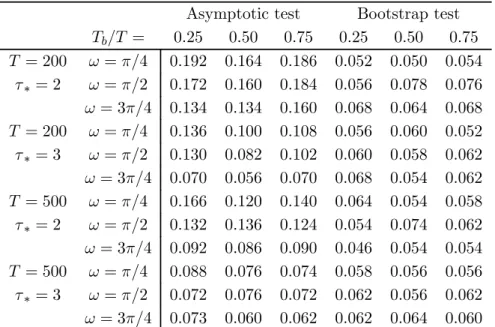
Table 1 shows the rejection frequencies of the tests at the 5% level when the DGP is given by the processes (17-18). We see that the rejection rates of the bootstrap test are always quite close to the nominal size. While we see, the asymptotic test tends to be oversized, especially when T = 200, τ∗ = 2, and Tb/T differs from 0.50. With T = 200 the bootstrap test is
better sized than the asymptotic one for all the eighteen experiments and fifteen differences between the rejection rates are indeed significant.5 Even with T = 500 the bootstrap test is less size-distorted in seventeen experiments and twelve differences between the rejection rates are significant. Interestingly, the empirical sizes of the two tests are more similar when the model is locally stable at frequency 3π/4.
Table 1: Rejection rates of 5% level tests under the null hypothesis of local stability at frequency ω
Asymptotic test Bootstrap test Tb/T = 0.25 0.50 0.75 0.25 0.50 0.75 T = 200 ω = π/4 0.192 0.164 0.186 0.052 0.050 0.054 τ∗ = 2 ω = π/2 0.172 0.160 0.184 0.056 0.078 0.076 ω = 3π/4 0.134 0.134 0.160 0.068 0.064 0.068 T = 200 ω = π/4 0.136 0.100 0.108 0.056 0.060 0.052 τ∗ = 3 ω = π/2 0.130 0.082 0.102 0.060 0.058 0.062 ω = 3π/4 0.070 0.056 0.070 0.068 0.054 0.062 T = 500 ω = π/4 0.166 0.120 0.140 0.064 0.054 0.058 τ∗ = 2 ω = π/2 0.132 0.136 0.124 0.054 0.074 0.062 ω = 3π/4 0.092 0.086 0.090 0.046 0.054 0.054 T = 500 ω = π/4 0.088 0.076 0.074 0.058 0.056 0.056 τ∗ = 3 ω = π/2 0.072 0.076 0.072 0.062 0.056 0.062 ω = 3π/4 0.073 0.060 0.062 0.062 0.064 0.060
In order to evaluate the effects of the break at frequencies π/4, π/2, and 3π/4 under the alternative hypothesis H1, Table 2 reports the spectra of the processes (15-16) at those
cies. It emerges that the effect of the break, as measured by the relative change in the spectrum at the frequency of interest, is the strongest at frequency 3π/4 and the weakest at π/4.
Table 2: Spectrum of model (16) Frequencies Break size π/4 π/2 3π/4 τ = 1 0.992 1.105 0.696 τ = 2 0.972 1.220 0.494 τ = 3 0.942 1.342 0.362 τ = 4 0.905 1.471 0.274
We report in Table 3 the rejection rates of both the asymptotic and bootstrap tests at the 5% level when the DGP is given by the processes (15-16).
Table 3: Rejection rates of 5% level tests under the alternative hypothesis of global instability
Asymptotic test Bootstrap test Tb/T = 0.25 0.50 0.75 0.25 0.50 0.75 T = 200 ω = π/4 0.222 0.206 0.200 0.068 0.064 0.068 τ = 2 ω = π/2 0.170 0.176 0.198 0.066 0.070 0.078 ω = 3π/4 0.282 0.256 0.234 0.144 0.136 0.112 T = 200 ω = π/4 0.278 0.286 0.206 0.114 0.184 0.146 τ = 3 ω = π/2 0.154 0.158 0.174 0.084 0.104 0.116 ω = 3π/4 0.360 0.400 0.296 0.274 0.336 0.230 T = 200 ω = π/4 0.432 0.538 0.404 0.272 0.512 0.372 τ = 4 ω = π/2 0.134 0.198 0.180 0.120 0.198 0.170 ω = 3π/4 0.636 0.672 0.456 0.608 0.690 0.456 T = 500 ω = π/4 0.264 0.236 0.192 0.126 0.136 0.088 τ = 2 ω = π/2 0.168 0.160 0.188 0.082 0.090 0.074 ω = 3π/4 0.312 0.348 0.286 0.172 0.226 0.158 T = 500 ω = π/4 0.502 0.614 0.438 0.416 0.596 0.412 τ = 3 ω = π/2 0.158 0.216 0.206 0.134 0.196 0.174 ω = 3π/4 0.692 0.800 0.600 0.638 0.778 0.572 T = 500 ω = π/4 0.888 0.968 0.863 0.878 0.968 0.851 τ = 4 ω = π/2 0.306 0.432 0.335 0.296 0.442 0.297 ω = 3π/4 0.954 0.966 0.942 0.944 0.972 0.934
Given the size distortions of the asymptotic test, caution is needed in comparing the em-pirical power of the two tests. However, the asymptotic test rejects more often in almost all the experiments. The two tests tend to have similar power as the parameters τ and T increase, as well as the null hypothesis is local stability at frequency π/4. For both the tests, it appears
that for a shock of 2 or 3 times the standard deviation of the residuals, the power is relatively low even if a large sample is considered. This result indicates that the size of the shock should be large enough to make the distinction between local and global stability. As in Candelon and Lütkepohl (2001), it is observed that the rejection frequency is generally lower when the break is located at the borders of the sample (i.e. Tb/T = 0.25, 0.75). The results reveal to us that
the frequency at which the break occurs is also important for the empirical power. As expected in view of Table 2, the power is the highest when the break occurs at frequency 3π/4.
5
Empirical applications
5.1
Output, consumption, and investment.
Several studies have been devoted to the analysis of the productivity slowdown in postwar U.S. output. As the univariate analysis of the output series by Bai et al. (1998) lead to inconclusive results, these authors considered a trivariate system composed of consumption (C), investment (I), and output (Y ). Following King et al. (1991), the rationale behind this idea is that a break in the productivity process should also be present in variables possessing strong long-run links with output, in particular consumption and investment. Indeed, Bai et al. (1998) proved that if the stochastic growth model by King et al. (1998) is augmented with a break in the average growth rate of productivity, such a break will affect the three variables c = ln(C), i = ln(I), and y = ln(Y ), but not the "great ratios" (c − y) and (i − y).
We thus investigate local and global stability in the following dynamic model:
A3(L) ct− yt it− yt ∆(ct+ yt+ it) = Φ3+ εt,
where A3(L) is a polynomial matrix of order 4,6 Φ3 is a vector of constant terms and εt are
N2(0, Σ) innovations. Quarterly data are obtained from the Saint-Louis Federal Reserve Bank
and cover the period 1954Q1-2004Q4. Yt is the private GDP per capita, Ct the real personal
consumption expenditures per capita, and It the private fixed investment per capita. The
variables are seasonally adjusted and divided by the civilian non-institutional population aged 16 and over.
The global stability test is implemented and the outcomes are reported in Table 4. Similar to Bai et al. (1998), a break is detected in 1968Q3. Interestingly, the break is dated earlier than the first oil shock.
6
The lag length is chosen according to the Akaike information criterion. Other choices of the lag length do not qualitatively modify the results.
Table 4: Stability Test H0 vs H1
break date statistic bootstrap p-value asymptotic p-value 1968q3 51.576 3.92% < 1.00%
Note: The bootstrap p-value is obtained after 5000 replications.
In order to gain a deeper insight into the origin of the break in 1968Q3, the local stability tests are performed for the frequencies ωj = (100j )π, for j = 1, 2, ..., 99. The tests statistics,
along with their bootstrap 95% and asymptotic critical values, are plotted in Figure 1.
Figure 1: Tests for local stability - The "great ratios" system
It turns out that this system is locally stable for frequencies higher than 1, i.e. with a wavelength lower than 6 quarters, but it becomes unstable at lower frequencies, in particular when ω approaches zero. This evidence suggests that the break in 1968Q3 can be labelled as "real" as it affects the long-run properties of the variables. However, unlike the prediction of the theoretical model by Bai et al. (1998), the stochastic components of the data are also unstable at low frequencies. Therefore, a simple break in the productivity average growth rate is not, apparently, the only origin of this break.
5.2
The predictive power of the yield curve on output growth
There is an extensive literature documenting the predictive power of the yield curve slope for future economic activity. Several factors can explain this stylized fact. As the yield curve
describes the relationship between yields and maturities, it is determined by financial markets’ expectation of future interest rate and the term premium. In front of a recession, the central bank may take the decision to stimulate activity, using the traditional instrument of monetary policy, i.e. by seeking to short-run interest rates. Consequently, the long-run interest rate will also decrease, but to a lesser degree, because of the expectations hypothesis of the term structure, leading to an increase in the yield curve. As the monetary expansion is expected to increase future activity, the correlation between the yield curve and future output growth is positive. The same relationship can be found using a Consumption Capital Asset Pricing model (Campbell and Cochrane, 1999), a Real Business Cycle model, or even a simple IS-LM model , see Estrella et al. (2003).
At an empirical level, several papers have provided evidence in favor of a positive correlation between the yield curve slope and future output growth in the United States.7 Nevertheless, Estrella and al. (2003) have questioned the stability of this relationship, finding evidence of a break around September 1983. They justify the presence of this rupture by the effects of the change in the US monetary policy. It became more oriented towards inflation control since the nomination in 1979 of Paul Volcker as the head of the Federal Reserve Bank.
For this example, we propose using the local stability test to investigate the stability of the predictive power of the yield curve slope on output growth in the US. We use monthly data of industrial production (IP ), 10-year treasury rate (10T T ), and the Federal fund rate (F F R) for the US economy, as extracted from the Saint-Louis Federal Reserve Bank. The sample covers the period 1955M1-2003M12. As IP presents unit roots, we compute the future growth rate of industrial production at a forecast horizon k (∆IPt,k) as:
∆IPt,k = (1200/k) ln(IPt+k/IPt) (19)
Since Estrella et al. (2003) showed that the predictable power of the spread is maximum at a horizon of one year, we also consider this horizon (k = 12) in the rest of the subsection. The interest rate spreads is given as the difference between the long-run and the short-run interest rate, i.e. Spread = (10T T − F F R). 8 We then build a bivariate VAR of the following form:
A4(L) Ã ∆IPt,12 Spreadt ! = Φ4+ ε1,t,
where A4(L) is a polynomial matrix of order 4,9 Φ4 is a vector of constant terms and ε1,t are
N2(0, Σ1) innovations.
The parameter stability of the above model will thus been investigated using the bootstrap
7See, inter alia, Estrella and Hardouvelis (1991), Plosser and Rouwenhorst (1994), Bonser-Neal and Morley
(1997), Kozicki (1997), Dotsey (1998), Breitung and Candelon (2005).
8
It has been checked that the results are robust if we consider the 3 − month treasury rate instead of the FFR. Results are available from authors upon request.
9
procedure for unknown breaks that was discussed in subsection 3.2. Table 5: Stability Test for H0 vs H1
break date statistic bootstrap p-value asymptotic p-value 1980.07 80.221 < 0.02% < 0.01%
Note: The bootstrapped p-value is obtained after 5000 replications.
It turns out that a break is detected in 1980M7. This break date is earlier than the one found by Estrella and al. (2003) in 1983M9. Nevertheless, our dating of the break seems more closely associated with the change in monetary policy regime associated with the appointment of Volcker as the head of the FED in late 1979. A possible explanation of the differences between our result and that of Estrella and al. (2003) is that we consider a bivariate system, whereas Estrella and al. (2003) investigate the stability of a single-equation model where future output growth is the endogenous variable.
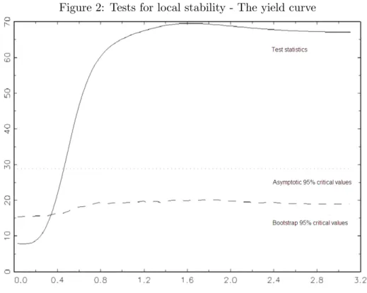
The study of global instability is then performed, it is possible to investigate the local stability around the break date that was previously obtained. Local stability tests are computed for the frequencies ωj = (100j )π, for j = 1, 2, ..., 99. In Figures 2, we plot the test statistics along
with their bootstrap and asymptotic 95% critical values.
Figure 2: Tests for local stability - The yield curve
It appears that the system is locally stable for frequencies lower than 0.3, i.e. for a wave-length longer than 21 months. This evidence is consistent with the view that this break has a
"nominal" origin. Indeed, the new orientation of the US monetary policy, being more concerned by inflation control, has apparently affected the stability of the spread/future output growth relationship at the higher frequencies while leaving unchanged the low-frequency components of the data.
6
Conclusions
In this paper, we develop a new testing procedure for parameter stability in a segmented stationary or cointegrated VAR model at a particular frequency. By doing so, it is possible to determine the range of frequencies which are responsible for the parameter instability in a dynamic model. The local stability tests can provide a deeper insight into the origin of a structural break. The two examples presented in this study highlight the practical value of this procedure in empirical studies. A structural break is detected at 1968Q3 in the case of an output-consumption-investment system, and around 1980M7 for the spread/future output growth relationship. The application of the local stability tests reveals that in the first case, the instability exclusively concerns the low frequency component of the data, whereas in the second case the model is only unstable at higher frequencies. From these characteristics, it follows that a real productivity shock is likely to be at the origin of the instability of the output-consumption-investment system, whereas a nominal shock, that being the change in the U.S. monetary policy in the early 80’s, has led to the modification of the predictive power of the interest rate spread for future output growth.
References
[1] Andrade, P., Bruneau, C. and S. Gregoir (2005), "Testing for Cointegration Rank when some Cointegrating Direction are Changing", Journal of Econometrics, 124(2), 2004, 269-310.
[2] Andrews, D.K (1993), "Tests for Parameter Instability and structural Change with un-known change Point", Econometrica, 61,4, 821-856.
[3] Bai, J. (2000), "Vector Autoregressive Models with Structural Changes in Regression Coefficients and in Variance-Covariance Matrices," Annals of Economics and Finance, 1, 303-339.
[4] Bai, J., Lumsdaine, R.L. and J.H. Stock (1998) "Testing for and Dating Breaks in Multivariate Time Series," Review of Economic Studies, 65, 395-432.
[5] Bai, J. and P. Perron (1998), "Estimating and testing linear models with multiple structural changes", Econometrica, 66,1, 47-78.
[6] Bai, J. and P. Perron (2003), "Computation and Analysis of Multiple Structural Change Models", Journal of Applied Econometrics, 18, 1-22.
[7] Bai, J. and P. Perron (2004), "Multiple Structural Change Models: A Simulation Analysis", forthcoming in Econometric Essays, D. Corbea, S. Durlauf and B.E. Hansen (eds.), Cambridge University Press.
[8] Bonser-Neal, C. and T.R. Morley, (1997), "Does the Yield Spread Predict Real Economic Activity?", Federal Bank of Kansas City Quarterly Review, Third Quarter. [9] Breitung, J. and B. Candelon (2005), "Testing for short- and long-run causality: A
frequency domain approach ", Forthcoming in Journal of Econometrics.
[10] Boulier, B.L. and H.O. Stekler, (1999), "The Term Spread as a Monthly Cyclical Indicator: An evaluation", Economics Letters, 66, 79—83.
[11] Candelon, B. and H. Lütkepohl, (2001), "On the Reliability of chow-type Tests for Parameter Constancy in Multivariate Dynamic Models", Economics Letters, 73, 155—160. [12] Centoni, M. and G. Cubadda (2003), "Measuring the Business Cycle Effects of Perma-nent and Transitory Shocks in Cointegrated Time Series", Economics Letters, 80, 45-51. [13] Chow, G.C. (1960), "Tests of equality between sets of coefficients in two linear
regres-sions", Econometrica, 28, 591-605.
[14] Christiano, L.J. and R.J. Vigfusson, (2003), "Maximum likelihood in the frequency domain: the importance of time-to-plan", Journal of Monetary Economics, 50, 789-815 [15] Diebold, C. and H. Chen (1996), "Testing structural stability with Endogenous
Break-point: A size Comparaison of Analytic and Bootstrap Procedure", Journal of Economet-rics, 70, 221—241.
[16] Dotsey, M. (1998), "The Predictive Content of the Interest Rate Term Spread for Future Economic Growth", Federal Bank of Richmond, Economic Quarterly, 84/3, Summer. [17] Estrella, A. and A. Hardouvelis, (1991), "The Term Structure as a Predictor of Real
Economic Activity", The Journal of Finance, 46, 555—575.
[18] Estrella, A., Rodrigues, A.P. and S. Schich, (2003), "How Stable is the Predictive Power of the Yield curve? Evidences from Germany and the United States", The Review of Economics and Statistics, 85, 629—644.
[19] Hansen, B.E. (2001), The New Econometrics of Structural Change: Dating Breaks in U.S. Labour Productivity, Journal of Economic Perspectives, 15, 117-128.
[20] Hansen, P.R. (2003), "Structural Changes in the Cointegrated Vector Autoregressive Model", Journal of Econometrics, 114, 261—295.
[21] Johansen, S. (1996), Likelihood-Based Inference in Cointegrated Vector Autoregressive Models, Oxford University Press.
[22] King, R. G., Plosser, C. I. and S. Rebelo, (1988), "Production, Growth and Business Cycles, II. New directions", Journal of Monetary Economics, 21, 309-342.
[23] King, R.G., Plosser, C.I., Stock, J.H. and M.W. Watson, (1991), "Stochastic Trends and economic Fluctuations ", American Economic Review, 81, 819-840.
[24] Plosser, C.I. and K.G. Rouwenhorst, (1994), "International Term Structures and Real Economic Growth", Journal of Monetary Economics, 33, 133-155.
[25] Qu, Z. and P. Perron (2004), "Estimating and testing structural changes in multivariate regressions", Department of Economics, Boston University Working Paper.
[26] Quandt, R.E., (1960), "Tests of the hypothesis that a linear regression system obeys two separate regimes", Journal of American Statistical Association, 55, 320-330.