A 2-dimensional computational model to analyze the effects of cellular heterogeinity on cardiac pacemaking

ALMA MATER STUDIORUM

_{– UNIVERSITÀ DI BOLOGNA}

CAMPUS DI CESENA

SCUOLA DI INGEGNERIA E ARCHITETTURA

CORSO DI LAUREA MAGISTRALE IN INGEGNERIA BIOMEDICA

A 2-DIMENSIONAL COMPUTATIONAL MODEL

TO ANALYZE THE EFFECTS OF CELLULAR

HETEROGEINITY ON CARDIAC PACEMAKING

Tesi in:

Bioingegneria molecolare e cellulare LM

Relatore:

_{Presentata da:}

Prof. STEFANO SEVERI

CHIARA CAMPANA

Correlatore:

Prof. ERIC SOBIE

Abstract vii

Introduction xi

1 Sinoatrial node: physiology and mathematical modeling 1

1.1 The cardiac conduction system . . . 2

1.1.1 Anatomy and functions of the SAN . . . 4

1.1.2 The cardiac action potential . . . 7

1.1.3 Pacemaker action potential . . . 10

1.1.4 Heart rhythm and cardiac arrhythmias . . . 12

1.2 Mathematical modeling of cardiac AP . . . 13

1.2.1 Single cell model of the rabbit sinoatrial node . . . . 16

1.2.2 Maltsev model . . . 18

1.2.3 Severi model . . . 19

1.2.4 Electrical propagation and cable theory . . . 20

1.3 Heterogeneity in the SAN . . . 21

2 Materials and Methods 23 2.1 1-dimensional model implementation in MATLAB . . . 24

2.2 Implementation of the models in CUDA . . . 28

2.2.1 A look inside the CUDA Programming Model . . . . 28

2.2.2 Maltsev tissue model . . . 32

2.2.3 Parameter randomization . . . 37

2.3 Simulations . . . 42

3 Results 45 3.1 1-D model results . . . 46

Potential Amplitude . . . 50 3.2.2 Control + non-excitable cells model . . . 59

Conclusions 67

Appendix A 69

Appendix B 81

Acknowledgments 87

L’azione meccanica del cuore `e possibile grazie al verificarsi di eventi elet-trici che interessano le cellule cardiache, propriet`a che classifica il tessuto cardiaco tra i tessuti eccitabili. L’evento elettrico `e il segnale che scatena la contrazione meccanica, inducendo un temporaneo incremento di cal-cio intracellulare, che, a sua volta, reca un messaggio di contrazione alle proteine contrattili della cellula. Per queste ragioni il processo che com-bina l’eccitazione elettrica alla funzione meccanica `e definito accoppiamento eccitazione-contrazione. Il sistema di conduzione atriale comprende il nodo seno-atriale (SAN) posizionato nel lato superiore destro del cuore e in grado di generare spontaneamente un segnale elettrico periodico ad una frequenza di 60-100 battiti al minuto. In seguito le fibre intra-nodali conducono l’impulso al nodo atrioventricolare, che rappresenta l’unica connessione elet-trica tra atri e ventricoli. Il segnale elettrico si propaga attraverso il tessuto cardiaco via gap junctions tra cardiomiociti e in ciascuno di questi induce un processo denominato potenziale d’azione (AP). La morfologia del poten-ziale d’azione cardiaco mostra un’elevata variabilit`a all’interno del cuore. Le cellule del SAN non possiedono un vero e proprio potenziale di riposo, bens`i generano regolarmente potenziali d’azione spontanei. A differenza dei potenziali d’azione non-pacemaker nel cuore, la corrente depolarizzante proviene principalmente da ioni Ca2+

piuttosto che da correnti di Na+

. Non vi sono infatti canali veloci di Na+

e relative correnti operanti nelle cellule nodali SA. Ci`o si traduce in un pi`u lento potenziale d’azione in termini di rapidit`a con cui le cellule si depolarizzano.

I meccanismi citati possono essere descritti e studiati sfruttando i principi della modellazione matematica, introdotta in ambito cardiaco in seguito al lavoro di Hodgkin e Huxley, i quali hanno presentato la descrizione matem-atica di correnti ioniche generanti AP nell’assone gigante di calamaro. Le equazioni di Hodgkin-Huxley (HH) costituiscono ancora oggi parte della

triche. Da allora, il numero di modelli formulati `e cresciuto rapidamente. In questa tesi sono presi in considerazione i due pi`u recenti modelli di singola cellula del nodo seno-atriale di coniglio (modello Severi (2012) e modello Maltsev (2009)).

Nella formulazione di modelli di singola cellula si considerano solamente le propriet`a medie del tessuto studiato, invece, per fornire una descrizione pi`u realistica, sarebbe utile considerare la variabilit`a normalmente presente all’interno del tessuto. Questo `e particolarmente vero nel caso del SAN, che ha una struttura molto complessa che mostra eterogeneit`a anatomica e fun-zionale. Come sar`a discusso pi`u avanti, questa variabilit`a pu`o dipendere da molteplici cause. `E possibile allora considerare modelli di cellule accoppiate utilizzando un array o una matrice e introducendo differenze nel compor-tamento di ogni singola cellula. In tal caso il comporcompor-tamento di ciascuna cellula `e influenzato da quella vicina, in particolare ogni cellula ricever`a un contributo in corrente dalle cellule adiacenti, che dipende dalla loro dif-ferenza di tensione e dalla resistenza di accoppiamento attraverso la legge di Ohm. Tale ragionamento `e noto come cable theory e pu`o essere esteso ad una propagazione multidimensionale, considerando un modello tissutale. Obiettivo principale del mio progetto `e stato l’implementazione in CUDA (acronimo di Compute Unified Device Architecture, un’architettura hard-ware per l’elaborazione parallela creata da NVIDIA) di un modello tissutale del nodo seno-atriale di coniglio attraverso il quale valutare l’eterogeneit`a della sua struttura e come tale variabilit`a influenzi il comportamento delle cellule. In particolare ogni cellula possiede una frequenza di scarica intrin-seca, dunque diversa da quella di ogni altra cellula del tessuto ed `e quindi interessante studiare il processo di sincronizzazione delle cellule e quale sia la frequenza ultima di scarica qualora queste risultino sincronizzate.

• Il primo passo `e stato realizzato utilizzando MATLAB per imple-mentare un modello monodimensionale del SAN di coniglio, descrivendo ogni cellula attraverso il modello Maltsev o Severi. Considerando un gruppo di cellule in fila, se ciascuna cellula `e regolata dalle stesse equazioni differenziali ed ha gli stessi valori per tutti i parametri, in ogni momento le cellule possiedono lo stesso potenziale di membrana e quindi hanno tutte la stessa frequenza di scarica. Ci`o si traduce in

di conduzione.

• Il resto del lavoro `e stato effettuato utilizzando CUDA e visualizzando poi i risultati in MATLAB. Grazie ai vantaggi introdotti dallo sfrutta-mento di unit`a di elaborazione grafiche (GPU) in termini di tempo di esecuzione, `e stato possibile creare un modello 2D del SAN di coniglio. • Tale modello `e stato infine utilizzato per esaminare la sincronizzazione e l’influenza reciproca tra le cellule. Dopo aver eseguito la random-izzazione di tutte le conduttanze massime presenti nel modello, sono stati valutati gli effetti sulla lunghezza del ciclo e l’ampiezza dei poten-ziali d’azione. Diversi livelli di accoppiamento resistivo tra cellule e di variabilit`a intercellulare delle conduttanze sono stati testati.

Le simulazioni effettuate utilizzando il modello realizzato suggeriscono che le cellule sincronizzano la loro frequenza di scarica. In particolare il valore ultimo della frequenza di scarica cresce al crescere della resistenza di accop-piamento e della variabilit`a intercellulare testate. L’ampiezza dei poten-ziali d’azione presenta un comportamento simile a quello della lunghezza del ciclo, diminuendo nel caso di aumento di resistenza di accoppiamento e variabilit`a intercellulare, anche se in maniera meno marcata nell’ultimo caso.

Il primo capitolo tratta il sistema di conduzione cardiaco, le caratteristiche del nodo seno-atriale e il potenziale d’azione delle cellule che lo costituis-cono per poi riportare i principi della modellazione cardiaca, con particolare riferimento alla descrizione della propagazione elettrica intercellulare. Nel secondo capitolo si discute l’implementazione dei modelli utilizzati in questo lavoro di tesi e sono descritte in dettaglio le simulazioni effettuate. L’ultimo capitolo riporta infine i risultati ottenuti dalle simulazioni, dedicando par-ticolare attenzione agli esiti delle simulazioni 2D, obiettivo primario del lavoro.

The mechanical action of the heart is made possible in response to electrical events that involve the cardiac cells, a property that classifies the heart tis-sue between the excitable tistis-sues. At the cellular level, the electrical event is the signal that triggers the mechanical contraction, inducing a transient increase in intracellular calcium which, in turn, carries the message of con-traction to the contractile proteins of the cell. For these reasons, the process that combines the electrical excitation to the mechanical function is called excitation-contraction coupling. The atrial conduction system includes the sinoatrial node (SAN) placed in the upper right corner of the heart able to spontaneously generate a periodic electrical signal at a frequency of 60-100 bpm; then intra-nodal pathways lead the impulse to the atrioventricular node, which is the only electrical connection between atria and ventricles. The electrical signal propagates in the cardiac tissue via gap junctions be-tween cardiac myocytes and in each myocyte it initiates a process named action potential (AP). The morphology of the cardiac action potential shows a high variability within of the heart. SAN cells are characterized as having no true resting potential, but instead generate regular, spontaneous action potentials. Unlike non-pacemaker action potentials in the heart, the de-polarizing current is carried into the cell primarily by relatively slow Ca2+

currents instead of by fast Na+

currents. There are, in fact, no fast Na+

channels and currents operating in SA nodal cells. This results in a slower action potentials in terms of how rapidly they depolarize.

The mentioned mechanisms can be usefully treated within the mathe-matical modeling. The first step towards mathemathe-matical modeling of car-diac cells was made after Hodgkin and Huxley presented the mathematical description of ion currents generating APs in the squid giant axon. The Hodgkin-Huxley (H-H) equations were later introduced to the field of car-diac APs, and the H-H formalism is still used as a part of nowadays carcar-diac

time, the number of different cell models has grown rapidly. In this thesis the two most recent rabbit SAN cell models (Severi model (2012), Maltsev model (2009)) are taken into account.

In formulating models of single cell, only the average properties of the tis-sue under inspection can be considered, instead to have a more realistic description it would be helpful to consider the variability normally present within the tissue. This is especially true in the case of the SAN, that has a very complex structure showing anatomical and functional heterogeneity. As discussed later, this variability may depend on multiple causes. It is pos-sible to consider models of coupled cells using an array or a matrix of cells and introducing differences in the behavior of each single cell. In that case the behavior of each cell is influenced by her neighboring, in particular each cell will receive a contribution in current from its neighbors, which depends from their voltage difference and from the coupling resistance through the Ohm’s law. This is known as the cable theory and it can be extended to a multidimensional propagation, considering a tissue model.

The primary goal of my project was to implement in CUDA (Compute Unified Device Architecture, an hardware architecture for parallel processing created by NVIDIA) a tissue model of the rabbit sinoatrial node to evaluate the heterogeneity of its structure and how that variability influences the behavior of the cells. In particular, each cell has an intrinsic discharge frequency, thus different from that of every other cell of the tissue and it is interesting to study the process of synchronization of the cells and look at the value of the last discharge frequency if they synchronized.

• The first step has been made using MATLAB to implement a 1-dimensional model of the rabbit sinoatrial node, describing each cell through the Maltsev or Severi model. Considering a cable of cells, if each cell is governed by the same differential equations and has the same values for all the parameters, at any moment the cells will be at the same potential and therefore have all the same rate. This results in a behavior of the cable which is identical to the behavior of the single cell.

• The rest of the work was carried out using CUDA and then displaying the results in MATLAB. Thanks to the advantages of CUDA in terms of execution time it was possible to create a 2-dimensional model of the rabbit SAN.

• This model was finally used to evaluate the synchronization and the mutual influence between cells. After having performed the random-ization of all maximal conductances, we evaluated the effects on cycle length and action potential amplitude. Different levels of resistive coupling between cells and inter-cellular variability of conductances were tested.

The simulations made using the tissue model show how cells synchronize their discharge frequency, and in particular the ultimate value of discharge frequency increases with the coupling resistance and the inter-cellular vari-ability. The action potential amplitude has a behavior similar to that of the cycle length, decreasing as coupling resistance and inter-cellular variability increase, although less markedly in the last case.

The first chapter describes the cardiac conduction system, the properties of the sinoatrial node and the action potential of his cells and then the principles of the cardiac modeling, with particular reference to the inter-cellular electrical propagation, are explained. The second chapter discusses the implementation of the models used in this thesis and the performed simulations. The last chapter finally outlines the results obtained from the simulations with particular attention to 2D simulations, primary goal of this work.

Sinoatrial node: physiology

and mathematical modeling

In this first chapter we introduce the background knowledge which has been necessary to carrying out the work of thesis. We start with a brief descrip-tion of the cardiac conducdescrip-tion system, focusing on the sinoatrial node, its physiological role and its anatomy. Then, talking about the cardiac elec-trical activity, we describe the cardiac action potential, making distinction between different cell types and focusing on the pacemaking activity and on the relation between action potential features and heart rhythm and the problem of cardiac arrhythmias. The second part explains the bases of the mathematical modeling in cardiac field, giving particular attention to the models studied for our project and to the mathematical representation of the anisotropic electrical propagation in cardiac physiology.

It was two centuries ago when for the first time Galvani and Volta proved spontaneous heart contractions to be related to electrical phenomena. These last events which take place within the heart give rise to the normal cardiac contraction and their alterations can cause severe cardiac rhythm disor-ders. The nervous system can command several heart properties, like its frequency and its force of contraction but heart functionality does not rely on its innervation. A denervated and transplanted heart is still able to work and adapt itself to different circumstances and this ability is due to some cardiac tissue intrinsic properties, its automaticity, i.e. the ability to au-tonomously initiate the heart beat and its rhythmicity, i.e. regularity of this autonomous activity [24].

The electrical signal coordinate the mechanical activity of the heart, a

four-Figure 1.1: Scheme of the cardiac conduction system [20].

chambered organ, consisting of two pumps: the right heart, which drives blood through the lungs and then back to the heart, forming the pulmonary circulation, and the left heart, that is responsible for the systemic circula-tion, driving the oxygenated blood around the body.

Cardiac tissue is a syncytium of cardiac muscle cells, each of which has a contractile capability similar to that of the skeletal muscle. Besides being contractile, cardiac cells are excitable, enabling action potentials to propa-gate, and the action potential causes the cells to contract, thereby enabling

the pumping of blood. We will discuss in detail later the features of cardiac action potential while for now we focus on the pathway of propagation of the electrical activity of the heart, shown in Fig. 1.1. It is initiated in a collection of cells known as the sinoatrial node (SAN) located just below the superior vena cava on the right atrium. The cells in the SAN are au-tonomous oscillators and the action potential generated by these cells is propagated through the atria by the atrial cells. The conduction of action potentials between atria and ventricles is normally prevented by a septum composed of non excitable cells and the action potential can continue its propagation only through a group of cells, known as the atrioventricular node (AVN) and located at the base of the atria. After having passed quite slowly through the AVN, the action potential propagates through the bundle of HIS composed by a specialized collection of fibers, named Purkinje fibers which spread via tree-like branching into the left and right bundle branches throughout the interior of the ventricles, ending on the endocardial surface of the ventricles. At this point the action potentials activate the ventricular muscle and propagate through the ventricular wall outward to the epicardial surface. The process whereby an electrical stimulus is converted into muscle contraction in ventricular cardiomyocytes is called Excitation-contraction (EC) coupling and its fundamental steps are shown in Fig. 1.2. L-type Ca2+

channels open as a result of the depolarization of the T-tubule by the action potential and they lead to an inward flow of Ca2+

ions (ICa). The

amount of Ca2+

entered the cell induces the sarcoplasmic reticulum (SR) to release additional Ca2+

through ryanodine receptors (RyR). This pro-cess is named Ca2+

-induced Ca2+

release (CICR). The released amount of Ca2+

diffuses through the myoplasm, binds to the myofilaments and causes contraction. It is then eventually removed from the myoplasm by ATPases, which pump the Ca2+

into the SR (sarcoplasmic reticulum Ca++

-ATPase (SERCA)) or out of the cell, or by the Na+

-Ca2+

exchanger (NCX), which transfers Ca2+

to the outside of the cell. Phospholamban (PLB) is a protein and the major substrate for the cAMP-dependent protein kinase (PKA) in cardiac muscle. In the unphosphorylated state it works as an inhibitor of the sarcoplasmatic calcium pump SERCA, while when phosphorylated by PKA its ability to inhibit SERCA is lost. When phospholamban is not phosphorylated, contractility and rate of muscle relaxation are decreased and this lead to decreasing stroke volume and heart rate, respectively. On the contrary, in case of sympathetic stimulation, for example, activators

Figure 1.2: Scheme of the major Ca2+

fluxes underlying Excitation-contraction coupling in ventricular cardiomyocytes. The inset shows the time courses of the action potential (AP), the Ca2+

transient, and the con-traction. AP happens first, followed by the Ca2+

transient and then by contraction [20].

of PKA, such as the beta-adrenergic agonist epinephrine can be released and this fact may enhance the rate of cardiac myocyte relaxation. In ad-dition, since SERCA is more active, the next action potential will cause an increased release of calcium, resulting in increased contraction (positive inotropic effect) [20].

1.1.1

Anatomy and functions of the SAN

As mentioned before, the sinoatrial node, located in the right atrium, serves as the primary site for initiation of the normal heartbeat (sinus rhythm). It was discovered over a century ago by Arthur Keith and Martin Flack as an anatomically defined tissue at the junction of the superior vena cava and right atria and today is recognized to be a distributed and heterogeneous complex adjacent to the crista terminalis with distinct regions defined by unique electrophysiological and structural properties. The SAN has a

cres-cent shape, it is 15 mm in length and 5 mm in width. It can be divided in two parts, one larger placed in the upper part of the right atrium and named head and one thinner, named tail and placed in the inferior right part [13]. In large animals, including the human, the node is functionally

Figure 1.3: Anatomy of the right atrium [3].

isolated with the exception of exit pathways that allow for communication between the SAN and atrial tissue. This insulation is made possible through the presence of a connective tissue, which is able to insulate the pacemaker’s automaticity from the hyperpolarizing electrical activity of the atrial my-ocardium. Another important feature of SAN found in multiple species is the presence of a centrally located artery around which the SAN cells are organized. These cells, weakly coupled between them, are heterogenous, in fact they comprise both pacemaker cells and non-pacemaker cells, such atrial myocytes, adipocytes and fibroblasts. The functional consequences of this great heterogeneity and its importance in our study are further dis-cussed later in this chapter, while here we focus on the morphology of SAN cells. Pacemaker cells found in the sinus node vary by size and electrophys-iological properties and can be divided into three different groups:

• elongated spindle shaped cells: cells which extend up to 80 µm in length and have a slightly striated cell body with one or more nuclei; • spindle cells: cells which have a similar shape to that of elongated spindle cells, but are shorter in length, extending up to 40 µm and are predominantly mono-nucleated;

• spider cells: cells which have irregularly shaped branches with blunt ends.

There is no clear understanding of the different cell types distribution, but experimental studies have shown that none of the three cell types have been found exclusively in a specific SAN area. In particular in the case of the rabbit SAN, which is our case of study, a uniform distribution of all the three pacemaker cell types has been observed in the central area.

Fig. 1.4 shows a schematic representation of these three types of cells. Also a representation of an atrial cell is illustrated, in fact in the crista terminalis region, atrial cells are the predominant cell type, together with a smaller

Figure 1.4: (A) Scheme on different types of SAN cells; (B)-(C) Schematic representation of two different models proposed to describe the transition from typical/central SAN (white ovals) to atrial (black ovals) cells: in (C) a gradual transition of intermediate cells (gray) from SAN center to crista terminalis is taken into account while in (B) a mosaic model is illustrated, the latter involves gradually decreasing ratio of SAN to atrial cell densities from SAN center to crista terminalis [32].

percentage of spindle nodal cells. Indeed the septal area of SAN is mostly composed of atrial cells and an almost uniform amount of the other three types of cells is interspersed between them. In the figure we can also see two different models proposed to describe the distribution of these different types of cells within the SAN. We will further discuss these two models later in this chapter [32].

1.1.2

The cardiac action potential

The electrical signal whose propagation has been briefly described before is named action potential and its general shape and phases for a ventricular cell are illustrated in Fig. 1.5. It is represented as the membrane potential waveform and it can be simply defined as a momentary change in electrical potential on the surface of a cell, especially of a nerve or muscle cell, that occurs when it is stimulated, resulting in the transmission of an electrical impulse. As in other cells, the cardiac action potential is a short-lasting event in which the difference of potential between the interior and the ex-terior of each cardiac cell rises and falls following a consistent trajectory, created by a sequence of ion fluxes through specialized channels in the mem-brane of cardiomyocytes that leads to cardiac contraction. While there are some differences in the action potentials of various types of cardiac tissue, discussed below, the following model is most commonly used for education purposes. Looking at the figure, we can distinguish five different stages:

• phase 4: resting phase. The typical resting potential in a cardiomy-ocyte is -90 mV, in this condition Na+

and Ca2+

channels are closed. • phase 0: depolarization. When an action potential triggered in a neighbouring cardiomyocyte or pacemaker cell causes the potential to rise above -90 mV, fast Na+

channels start to open and Na+

can en-ter the cell, further raising the membrane potential. The large Na+

current rapidly depolarizes the potential to 0 mV and slightly above 0 mV for a transient period of time called the overshoot, then fast Na+

channels close. Another type of channels playing during this phase is L-type (long-lasting) Ca2+

channels which open when the membrane potential is greater than -40 mV and cause a small but steady influx of Ca2+

.

Figure 1.5: Action potential waveform in a ventricular cell, (TMP=transmembrane potential) [18].

return to its original resting state. The cell can not depolarize again until this happens. Phases 1-3 are the repolarization phases and co-incide with the time that the cell is refractory and can not respond to a new stimulus.

• phase 1: early repolarization. At the beginning of this phase the mem-brane potential is slightly positive, then some K+

channels open briefly and an outward flow of K+

returns the potential to approximately 0 mV.

• phase 2: plateau phase. This is the distinguishing phase of the cardiac AP and it is cause of its long lasting. During this stage there is an equilibrium between inward and outward currents, in fact L-type Ca2+

channels are still open and there is a small, constant inward current of Ca2+

, and different types of K+

outward currents. The inward and outward currents are electrically balanced, so that the membrane potential is maintained at a plateau just below 0 mV throughout phase 2.

• phase 3: repolarization. This phase starts with the gradual inacti-vation of Ca2+

. The outflow of K+

instead is still present and now, exceeding Ca2+

resting potential of -90 mV to prepare the cell for a new cycle of depolarization.

The described ionic flows change the normal transmembrane ionic con-centration gradients, that must be restored, especially by returning Na+

and Ca2+

ions to the extracellular environment, and K+

ions inside of the cell. This is made primarily through the sarcolemmal Na+

-Ca2+ exchanger, Ca2+ -ATPase and Na+ -K+ -ATPase [15].

The primary cardiac cell types are: nodal cells (SAN cells and AVN cells),

Figure 1.6: Action potential waveform throughout the heart [15]. Purkinje fiber cells, and atrial and myocardial cells. Each cell type has a slightly different function, we already know that the primary function of SAN cells is to provide a pacemaker signal for the rest of the heart, the AVN have to transmit the electrical signal from atria to ventricles with a delay, Purkinje fiber cells are responsible for fast conduction, for the activation of the myocardium, and finally myocardial cells, both atrial and ventricular, are muscle cells, so that they are both contractile and excitable. The differ-ent functions of differdiffer-ent cardiac cell types lead these cell to have differdiffer-ent action potential shapes, however all are noticeably different than the neural action potential, in particular they have a long plateau phase which facili-tates and controls muscular contraction and cannot be found in the neural cells. Fig. 1.6 shows typical action potentials for several cell types.

cells and myocardial cells have substantially prolonged action potentials (300 - 400 ms compared to 3 ms for the squid axon). Even within a single cell type, there can be substantial variation. For example, in the ventricles, epicardial, midmyocardial, and endocardial cells have noticeable differences in action potential duration [20].

1.1.3

Pacemaker action potential

Cells of the sinoatrial node, on which we focus, have the property of auto-maticity thanks to their unique electrophysiological profile, that is distinct from that in atrial or ventricular cells. These latter are characterized as having a stable rest potential, while the SAN AP lacks a true resting po-tential due in large part to lack of the inward rectifier K+

channel IK1. The

SAN AP reaches a maximum diastolic potential (MDP) of about -60 mV, followed by a spontaneous depolarization that eventually reaches thresh-old to generate another AP, therefore the SAN is able to generate regular, spontaneous action potentials. Unlike most other cells that elicit action potentials (e.g., nerve cells, muscle cells), the depolarizing current is carried primarily by a relatively slow, inward Ca2+

current instead of by fast Na+

currents. In fact pacemaker cells have fewer inward rectifier K+

channels than do other cardiomyocytes, so their membrane potential is never lower than -60 mV. As fast Na+

channels need a transmembrane potential of -90 mV to reconfigure into an active state, they are permanently inactivated in pacemaker cells so there is no rapid depolarization phase. Pacemaker cells have an unstable membrane potential and their action potential is not usually divided into the same defined phases seen before.

Fig. 1.7 shows a typical AP of a SAN cell, the different phases and the in-volved currents are indicated. The sequence of events for pacemaker action potential are:

• phase 4: spontaneous depolarization, which leads the membrane po-tential to overcome the threshold level. At the end of the repolar-ization, when the membrane potential is really negative, i.e. the maximum diastolic potential (MDP=the lowest membrane potential reached by the cell)) is about -60 mV, the funny current (If) is

ac-tivated. The latter is a distinguishing current of the nodal tissue, it is carried both by Na+

and K+

ions and it is activated by repolar-ization/iperpolarization, which starts at about -50 mV. The reversal

Figure 1.7: SAN cell Action Potential and currents involved in the different phases [21].

potential of the involved ionic channels is -10/20 mV, due to the their mixed permeability. The activation of this current, together with the increased activity of the sodium-calcium exchanger is responsible of the diastolic depolarization (DD). In particular this phase can be divided into two stages, the first one, called early diastolic depolar-ization primarily relies on the presence of the funny current, while the exchanger is more active in the second part, late diastolic depo-larization, immediately before systole. At the end of this phase the membrane potential is closer to the threshold, so almost ready for the upstroke;

• phase 0: depolarization of the AP (upstroke). Once the membrane potential has reached the threshold level (about -50/-40 mV), a rapid depolarization can start and move the membrane potential to a peak of about +20 mV. During this phase the conductivity of calcium chan-nels increases and we have two different types of inward currents, ICaL,

which is the largest contributor to the upstroke, and ICaT, which is

the first one to be activated (already at the end of phase 4). So the primary current during this stage is carried by Ca2+

flowing through L-type channels, for this reason the slope of phase 0, and so the speed of depolarization, is lower than the one found in the other cardiomy-ocytes;

• phase 3: repolarization. Once the membrane potential has reached positive values, K+

currents: IKr and IKs, which, together with the inactivation of ICaL,

return the membrane potential to negative values.

1.1.4

Heart rhythm and cardiac arrhythmias

Cardiac arrhythmias are disruptions of the normal cardiac electrical cycle and they are generally of two types. There are temporal disruptions, which occur when cells act out of sequence, either by firing autonomously or by refusing to respond to a stimulus from other cells, as in AVN block or a bundle branch block. A collection of cells that fires autonomously is called an ectopic focus. These arrhythmias cause little disruption to the ability of the heart muscle to pump blood, and so if they do not initiate some other kind of arrhythmia, are generally not life-threatening.

The second class of arrhythmias are those that are reentrant in nature and can occur only because of the spatial distribution of cardiac tissue. If they occur in the ventricles, reentrant arrhythmias are of serious concern and life-threatening, as the ability of the heart to pump blood is greatly di-minished. Reentrant arrhythmias on the atria are less dangerous, since the pumping activity of the atrial muscle is not necessary to normal function with minimal physical activity, although long-lived atrial reentrant arrhyth-mias are known to increase the chance of strokes. A reentrant arrhythmia is a self-sustained pattern of action potential propagation that circulates around a closed path, reentering and reexiting tissue as it goes. A classic example of a one-dimensional reentrant rhythm of clinical relevance is one in which an action potential circulates continuously between the atria and the ventricles through a loop, exiting the atria through the AV node and reentering the atria through an accessory pathway (or vice versa). Reen-trant patterns which are not constrained to a one-dimensional pathway are much more problematic. The two primary reentrant arrhythmias of this type are tachycardia and fibrillation. Both of these can occur on the atria (atrial tachycardia and atrial fibrillation) or in the ventricles (ventricular tachycardia and ventricular fibrillation). When they occur on the atria, for the reasons mentioned before, they are not immediately life-threatening, while when they occur on the ventricles, they are life-threatening. Ven-tricular fibrillation is fatal if it is not terminated quickly. Tachycardia is often classified as being either monomorphic or polymorphic, depending on the assumed morphology of the activation pattern. Monomorphic

tachy-cardia is identified as having a simple periodic ECG, while polymorphic tachycardia is usually quasi-periodic, apparently the superposition of more than one periodic oscillation. A typical example of a polymorphic tachy-cardia is called torsades de pointes, and appears on the ECG as a rapid oscillation with slowly varying amplitude (Fig. 1.8). Stable monomorphic ventricular tachycardia is rare, as most reentrant tachycardias degenerate into fibrillation [20].

Figure 1.8: A six-lead ECG recording of torsades de pointes [20].

1.2

Mathematical modeling of cardiac AP

Most part of the work made in cardiac modeling field derives from the experiments performed by Hodking and Huxley in the early ’50s. They were working on the squid giant axon using for the first time a technique, named patch-clamp, which then became crucial during the following years. With this technique the cells and their ionic channels are given particular voltage or current trajectory and then the resulting electrical activity is recorded. We can use different protocols, depending on the shape or type of trajectory used to stimulate the cell. The most common examples are: voltage clamp, current clamp and AP clamp. The latter does not use a fixed value of voltage or current but the cells are stimulated by a voltage profile reconstructed on the basis of a normal action potential. In their pioneering work, Hodking and Huxley recorded multiple electrical currents across the membrane and they identified an electric analogy to describe the cell membrane. From the circuit shown in Fig. 1.9 it derives that the

Figure 1.9: Electric analogy used to represent the cell membrane, the phospholipid bilayer is described as an electric capacitance C and the ionic channels through an electric resistance R [4].

currents playing a role in the action potential generation can be described mathematically by the following equation:

Cm∗

dVm

dt = −Im (1.1) where Cm is the electric capacitance of the cell, Vm is the voltage difference

across the cell membrane and Im is the sum of all the currents flowing

across the cell membrane. In turn each one of these currents is described mathematically by the following equation:

Iion = x ∗ gion∗ (Vm− Eion) (1.2)

where:

• x is the gating variable, i.e. an adimensional value in the range 0÷1, which represents the ratio of open channels at a certain instant in time. We could have more than one gating variable to represent a single channel. The mathematical description of a gating variable is discussed later;

• gion is the electrical conductivity of the ionic channel;

• Vm-Eion is called driving force, Eion is the reversal potential of the

considered ion (also known as the Nernst potential), i.e. the membrane potential at which there is no net flow of that particular ion from one

side of the membrane to the other. Eion is determined by the Nernst equation: Eion = R ∗ T Z ∗ F ∗ log [ion]i [ion]o (1.3) where:

– ion is the considered specific ion; – R=8.314472 J K−1

mol−1

, universal gas constant; – T temperature in Kelvin;

– Z valency of the element; – F=96485.3399 C mol−1

, Faraday constant; – [ion]i intracellular ion concentration;

– [ion]e extracellular ion concentration.

Gating variables are described by differential equations. Conductivity val-ues reached by some channels at fixed potential valval-ues are determined by performing clamp experiments, until the maximal conductivity is reached. These found values are then expressed in relative terms, giving a value to the gating variable for each one of the tested potentials. The resulting pa-rameter is named x∞ and it is defined by a voltage dependent equation.

The ionic channels require a certain amount of time to reach the x∞ value

(steady state value), so that we can define a time constant τx, which is

still voltage dependent. The equations for both parameters come from an interpolation of experimental data and they are the following:

x∞= α α + β (1.4) τx = 1 α + β (1.5) where α and β decribe the relationship with voltage, usually in an expo-nential form. Finally the expression for the voltage gating is the following:

dx

An equal alternative way is: dx dt = x∞− x τx (1.7) During the years a great number of cardiac cell models have been formu-lated, in this work we focus upon rabbit SAN cell models.

1.2.1

Single cell model of the rabbit sinoatrial node

The first sinoatrial node cell model was published in 1980 by Yanagihara, Noma and Irisawa. The model uses a HodgkHuxley formulation and in-cludes five trans-membrane currents: the Na+

, slow inward (Ca2+

), delayed rectifier K+

, hyperpolarization-activated, and time-independent leak (back-ground) currents. In this model, the slow inward current is responsible for the rising phase of the action potential and the plateau, determined by both slow inward current inactivation and activation of the dynamic K+

current [19].

After this first one, many other models have been proposed with the aim of including always more details. We carefully describe two of the most recent rabbit SAN cell models: Maltsev and Severi models, because they are the ones from which we start the implementation of our models and also because they describe the diastolic depolarization phase through two different hypotheses: membrane clock and calcium clock.

The properties of funny channel seem specifically apt to generate the di-astolic depolarization phase of the action potential, which is the phase re-sponsible for normal spontaneous activity. Because the membrane ionic channels open and close according to the membrane potential, this process is referred to as a membrane voltage clock. As mentioned before, If

acti-vates upon hyperpolarization, one of the unusual features which at the time of its discovery made the current deserve the attribute funny, at a threshold of about -40/-50 mV, and is fully activated at about -100 mV. In its range of activation, which quite properly comprises the voltage range of diastolic depolarization, the current is inward, its reversal occurring at about -10/-20 mV. This is due to the mixed Na+

/K+

permeability. The channels are encoded by the hyperpolarization-activated, cyclic nucleotide-gated (HCN) channel gene family. Of the four known HCN subunits, HCN4 is the most highly expressed in the mammalian SAN. The major role of If has been

reinforced by the fact that mutations in the If channel are associated with

a reduced baseline heart rate, and drugs, which block If (such as

ivabra-dine) do the same. Funny channels are so a successful target of specific heart-rate-reducing agents like ivabradine, and is known that funny current plays a key role on the pacemaking activity of heart cells.

The second hypothesis relies on the recent finding of spontaneous Ca2+

Figure 1.10: In the left part of the figure: membrane clock (If)

hypothe-sis: Simulated AP using the Severi model. In the right part of the figure: calcium clock hypothesis: Simulated AP using the Maltsev model [29]. release from the sarcoplasmic reticulum (SR), which has been suggested to be the mechanism for sinus rhythm generation. When the SR is full, the probability of spontaneous Ca2+

release increases. On the other hand, when the SR is empty, the chances for spontaneous Ca2+

release decrease. The rhythmic alteration of SR Ca2+

release is referred to as the Ca2+

clock. Because the SR Ca2+

content is controlled in part by the membrane volt-age, it is important to recognize that the activation of the Ca2+

clock and the membrane ionic clock are interdependent. Based on evidence from iso-lated SAN myocytes, late diastolic Cai elevation (LDCAE) relative to the

action potential upstroke is a key signature of pacemaking by the Ca2+

clock. On these bases a new modeling approach starts to be considered, in which rate regulation is governed by intracellular Ca2+

cycling and its coupling to the surface membrane. These new models differ from classical pacemaker models, which attribute the rate regulation of SAN cells mainly to the If activation state and its relation to the early DD slope. The rate

and amplitude of SR Ca2+

by the amount of free Ca2+

in the system, the SR Ca2+

pumping rate and the numbers of activated Ryanodine Receptors (RyR) [14].

1.2.2

Maltsev model

Figure 1.11: Schematic diagram of the interacting Ca2+

clock and mem-brane clock in the Maltsev model of rabbit sinoatrial node cells [29].

In contrast to earlier membrane-delimited models of the SAN cell, in 2009, Maltsev and Lakatta first developed a model of a coupled membrane-and Ca2+

-clock to address the ionic mechanism of cardiac pacemaking. Im-portantly, they quantitatively described the contribution of spontaneous Ca2+

release during late DD to SAN pacemaking, by triggering an inward Na+

-Ca2+

exchange current (IN CX). They concluded that only a coupled

system of membrane- and Ca2+

-clocks offers both the robustness and flex-ibility that are required to maintain normal pacemaking function. The Maltsev model predicts that the most important pacemaker current dur-ing late DD is the inward IN CX, instead of If. IN CX is the leading current

during the DD, and is secondary to dynamic changes in [Ca]i and the Ca2+

-clock. Without the Ca2+

-clock, the membrane-clock alone is not capable of maintaining normal pacemaking function.

This model is a system of 29 first-order differential equations. To avoid a lengthy transitional process, they set initial conditions for membrane clock gating variables to ready-to-fire status.

1.2.3

Severi model

In 2012, Severi et al. developed an updated model of a rabbit SAN cell based on the most recent experimental data, with an updated representation of intracellular Ca2+

dynamics. If remains the major pacemaker current in the

Severi model, and it is formulated using a similar Hodgkin-Huxley scheme. As predicted by the Severi model, If and the Na+-Ca2+ exchange current

IN CX are of similar size during DD. Yet If gradually increases to promote

depolarization, while the inward IN CXdecays slightly over time. In addition,

the model predicts that complete blockade of If will lead to cessation of

cell automaticity. In fact an outstanding improvement with respect to the Maltsev model, is its ability in reproducing the experimental effects of the If reduction, in particular the AP rate decrease, experimentally observed

in response to a partial If blockade. The Severi model reproduces an AP

rate decrease of 22% in case of a 66% If blockade; on the contrary, Maltsev

model is able to reproduce only a small reduction of the AP rate (about 5%) if If is completely blocked. If is described as composed of two relatively

independent Na+

and K+

components, If N a and If K, whose contributions

to the total conductance at normal Na+

and K+

concentrations, are similar. If is also modulated by the extracellular potassium concentration Ko.

This model is a system of 34 first-order differential equations.

1.2.4

Electrical propagation and cable theory

In this work of thesis the single cell model is only a starting point, then we will work on systems of coupled cells, either along a line or in a matrix. For this reason in this section we want briefly explain how to mathematically represent an action potential propagating down a uniform cable. First of all the cable must be divided into discrete segments so that we can analyze the cable as coupled equivalent circuits (Fig. 1.13). In the illustration we

Figure 1.13: One dimensional cable theory [34].

can see the mathematical circuit used to represent a single segment of the cable, which is the same we already described in the previous section. Then this circuit is replicated and coupled to other equivalent circuits to describe all the cable. These circuits are connected between them by a resistance Ri,

which corresponds to the intra-cellular resistance (for simplicity we assume extra-cellular resistance Re=0), while Vj represents the voltage at the jth

element of the cable. Said that and using the Ohm’s law and the Kirchoff’s current law, we can write the equations that describe the jth element of the cable: Ij−17→j = (Vj−1_{− V}j)/Ri (1.8) Ij7→j+1_{= (V}j − Vj+1_)/R i (1.9) Ij−17→j = Ij7→j+1+ AImj (1.10)

where Im is a current density and A is the surface area of the jth element

and Ij−17→j _{is the current flowing from the (j-1)th element to the jth element.}

area) can be written as follows: Ij m = Cm dVj dt + I j ion (1.11)

Now, putting the equations together, we obtain: (Vj−1 − Vj_)/R i = (Vj− Vj+1)/Ri+ A[Cm dVj dt + I j ion] (1.12)

and, rearranging the fields: Cm

dVj

dt = (V

j−1

− 2Vj) + Vj+1/ARi− Iionj (1.13)

The parameter Ri can be also related to cable geometry, in fact defined ρi

the intracellular resistivity, a the radius of the transversal section and ∆x

the length of each segment of the cable, we have: Ri=ρi∆x/πa2.

The approach of the cable theory to describe AP propagation can be easily extended to a multidimensional propagation. In this last case we should con-sider that transverse propagation means encountering more gap junctions per unit length and thus the resistance in this direction should be greater than the longitudinal one. The resistance value in fact is determined both by cardiac structure and gap junctions, although the cytoplasmic resistance is relatively low compared with the resistance encountered at gap junctions [34].

1.3

Heterogeneity in the SAN

A fundamental limit of single cell models is that they are unable to describe the interaction between cells and the variability normally existent between cells of they same organ. In fact each parameter present in the model is given an average value, which cannot take into account slight differences within the tissue. In this section we describe the great morphological and functional heterogeneity of the rabbit sinoatrial node, pointing out the most relevant aspects to this work of thesis.

Measurements from intact rabbit SAN have shown heterogeneity of electro-physiological properties from the center to the border of the atrium includ-ing gradual morphological changes in action potential, a decrease in maxi-mum diastolic potential, an increase in peak overshoot potential (POP), an

increase in upstroke velocity (UV) and a decrease in pacemaker potential slope. On the basis of these results, as described in the work of Oren et al. [28], two distinct hypotheses have arisen to explain intact SAN hetero-geneity. The first is that the SAN has two specific cell types, central cells and peripheral cells, each with distinct electrophysiological characteristics. The second hypothesis suggests that all observed heterogeneity in the intact SAN results from electrotonic coupling effects, i.e. cells in the SAN near the atria will be strongly affected and modified by the atrium. However what Oren et al. concluded from their tissue model simulations is that atrial electrotonic effects is plausible to account for SAN heterogeneity, sequence, and rate of propagation. They also have studied the effect of fibroblasts, concluding that they can act as obstacles, current sinks or shunts to con-duction in the SAN depending on their orientation, density, and coupling. Some of the most important hypotheses proposed to explain the observed heterogeneity of the rabbit sinoatrial node are summarised below:

• SAN tissue has fibroblasts interspersed in islands that occupy about 50% of SAN volume and they can act as obstacles, current sinks or shunts to conduction in the SAN depending on their orientation, den-sity and coupling;

• Verheijck et al. [11] have observed atrial cells interspersed in the SAN and suggested a mosaic model of SAN and atrial cells for SAN organization;

• Gap junction density and conductance increase moving from the cen-ter to the pheriphery of the SAN;

• SAN has two specific cell types, central cells and peripheral cells, each with distinct electrophysiological characteristics;

• All observed heterogeneity in the intact SAN results from electrotonic coupling effects, cells in the SAN near the atria will be strongly af-fected and modified by the atrium.

Materials and Methods

Starting from the single cell models for the rabbit sinoatrial node: Severi model and Maltsev model, first a 1D model both in MATLAB and CUDA and after a 2D model in CUDA were implemented. The 1D model, or ca-ble model consists of an array of cells placed along a line and connected between them and it was used to perform a comparison between the exe-cution time in MATLAB and CUDA, running the same simulations with both softwares. It was also handled to study and better understand the relationship between the cells coupling and the conduction velocity within a cable of cells. The 2D model, or tissue model consists instead of a matrix of cells and each one, except the ones on the boundary, is connected to four other cells. This last model has been useful in introducing in this study the heterogeneity of the SAN through a randomization of all the conductances existent in the Maltsev model, so that each cell had a different behavior and it was possible to evaluate how each one influences the others.

Therefore in this chapter we expose the steps taken for the implementa-tion of the instruments and the last secimplementa-tion briefly describes the performed simulations.

MATLAB

The Maltsev and Severi single cell models for the rabbit sinoatrial node, described in details in the previous chapter, were the starting point of my work. In the cable model we consider a group of cells placed along a line and connected between them through gap junctions, therefore, to pass from a single cell model to a cable model, each differential equation existent in the model and describing the evolution in time of a state variable must be replicated for each cell of the cable. In this thesis we have looked at cables of both 25 and 50 cells. The differential equation describing the evolution of the cell’s membrane potential was modified according to the cable theory to include the contribution in current each cell gives to the two neighboring cells. No-flux boundary conditions were considered.

The voltage equation that appears in the single cell model as:

dVm = −itot/Cm (2.1)

is then converted to the following:

dVm = −(itot/Cm) + Vnet/(Rgap∗ Cm) (2.2)

In the previous equations as usual Cm represents the cell’s membrane

ca-pacitance and it is equal to 32 pF, Vm is the membrane potential, expressed

in mV and itot, expressed in pA, is the sum of all the different currents used

in the model, respectively for the Maltsev and Severi model:

itot = iCaL+iCaT+if+ist+iKr+iKs+ito+isus+iN aK+iN aCa+ibCa+ibNa (2.3) itot = if+ibNa+ibCa+iKr+iKs+ito+iN aK+iN aCa+iN a+iCaL+iCaT+ibK+iKACh

• Rgap: this parameter takes into account the coupling strength between

the cells. It has the units of measurements of an electrical resistance, increasing its value the current contribution between the cells is de-creased according to the Ohm’s law. Its importance in this study will be further discussed later in this chapter and in the next one;

• Vnet: this parameter takes into account the difference in voltage

be-tween the cells, therefore it is expressed in mV and it is obtained as follows:

Vnet = Vm([2 : end, end]) − 2 ∗ Vm+ Vm([1, 1 : end − 1]) (2.5)

The resulting models are composed of systems of ordinary differential equations (ODE). MATLAB has a number of tools for numerically solving ODE, in our case we used the built-in function ode15s, which is one of the solvers designed for stiff problems, namely when ODE are such that the nu-merical errors compound dramatically over time. In general in that cases it is necessary to take considerably smaller steps in time to solve the equations, and this can lengthen the time to solution dramatically. Often, solutions can be computed more efficiently using one of the solvers specific for stiff prob-lems.

I first considered the cells governed by the same differential equations and with the same values for the parameters and the initial conditions of the state variables. The cells, having at each moment the same voltage, do not exert any influence on each other, in fact the contribution in current deriving from the Ohm’s law is equal to zero, the value given to Rgap does

not have any effect and the cells behave as a single one.

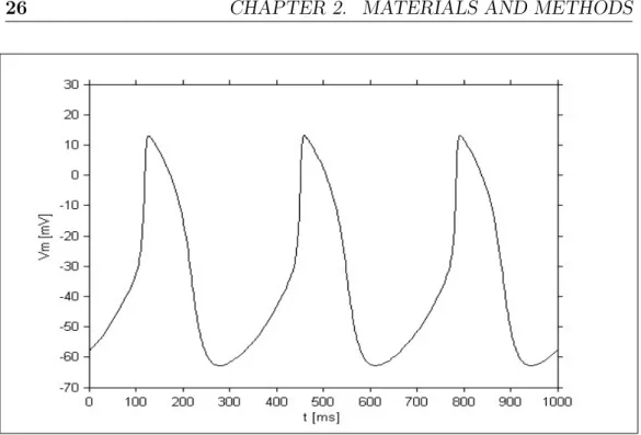
Figures 2.1 and 2.2 show the results obtained in this condition using the two models, obviously the results are the same considering a cable of either 25 or 50 cells.

Figure 2.1: Simulated AP using the Maltsev cable model

ditions have subsequently been changed to evaluate the effect of different values of Rgap over the conduction velocity within the cable. Each cell

was given different initial conditions for the state variables according to hypotheses made referring to the estimated physiological values of conduc-tion velocity in the rabbit SAN. Realistic values for the initial condiconduc-tions of the models state variables can be determined by using the usual relation between time, displacement and velocity (velocity=displacement/time). In our case the displacement is the distance between two neighboring cells within the cable and, using the relation above, it results that, considering average values for velocity and distance equal respectively to 10 cm/s and 100 µm, the time taken by the impulse to pass from one cell to the next is roughly equal to 1 ms. On the basis of these considerations, the initial conditions were in practice computed running simulations of the single cell models. To assign the initial conditions to the first cell of the line, a 50 s simulation was performed, the final values of the state variables become the initial conditions for this cell and they are stored in the first line of a matrix. Starting with these values as initial conditions, another simulation was performed, but this time the length of the simulation corresponds to the time delay between the two cells, so it is equal to 1 ms. As before the ending values of the state variables become the initial conditions for this cell and the conditions from which to start for the subsequent simulation. Repeating these same steps for the total number of the cells, all the initial conditions are assigned.

The simulations conducted using these instruments and their results are presented later.

Although the implementation of the cable model has been an important tool for learning the mechanism of connection between cells and the nec-essary steps to take to pass from single cell models to models of coupled cells, the primary purpose of my project was the implementation of a tissue model of the SAN. In order to do that we made use of CUDA, that enables huge improvements in computing performances thanks to the power of the graphic processing units (GPU). GPU’s parallel structure allows a very ef-fective manipulation of many parallel tasks rather than serial tasks. The code written in CUDA implements both a cable and a tissue model of the SAN, even if the 1D model has only been used to evaluate the advantages introduced in term of execution time comparing to MATLAB. The tissue model in CUDA has been realized considering only the Maltsev model to describe the cells, this choice has been supported by practical time reasons, but the same study could be made considering the Severi model, indeed it would be interesting to compare the results obtained in the two situations.

2.2.1

A look inside the CUDA Programming Model

First of all the program is divided into several phases that are executed on either the host (CPU) or the device (GPU) depending on the amount of data parallelism that they exhibit. Both host and device code are enclosed by the same source code, which is then compiled using the NVIDIA C Compiler (NVCC). At this point the two codes are separated, the host code is compiled with the host’s standard C compilers while the device code is further compiled by the NVCC and executed on a GPU device.

Therefore in our case the code, named Maltsev.cu, will be compiled from the command line by typing the following sequence:

nvcc -arch=sm 13 -o a Maltsev.cu The executable file is then executed through the line:

a.exe

The device code uses keywords for labeling data-parallel functions, called kernels, and their associated data structures. In particular a kernel, defined

allel, generates thousands of threads to exploit data parallelism.

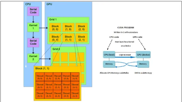
As described in fig.2.3 the execution of a typical CUDA program starts

Figure 2.3: Scheme of execution of a CUDA program

with host (CPU serial code) execution, then, if a kernel function is invoked, the execution is moved to the device (GPU parallel kernel). A kernel, dur-ing an invocation, as said before, generates a large number of threads and all these collectively form a grid. When all threads of a kernel complete their execution, the corresponding grid terminates and the execution con-tinues on the host until another kernel is invoked. Each kernel is involved in the performance of an individual part of the process and inside it specifies the code to be executed by all threads of a parallel phase. The following example shows a kernel code used in our program:

global void initialConditions(double* vars, int num param, int num cells, int cells per thread) _{

double Vm = -57.9639 ;

... other 27 variables are defined ... double RI = 0.31195 ;

... for all 29 parameters

int idx = threadIdx.x*cells per thread; int simulations = blockIdx.x;

int limit = idx+cells per thread; for (;idx<limit;idx++) {

vars[(simulations*num param*num cells) + idx +(0*num cells)] = Vm; ... other 27 values are assigned ...

vars[(simulations*num param*num cells) + idx +(28*num cells)] = RI; }

}

The syntax is ANSI C with some extensions, in fact there is a CUDA spe-cific keyword global , which starts the code and the declaration of each kernel in general and it indicates that that particular function is a kernel and so it can be called from a host function to generate a grid of threads. Other extensions used in CUDA and shown in the example are the key-words threadIdx.x and blockIdx.x, that refer, respectively, to the indices of a thread and of a block in which threads are grouped together. These subdi-visions and indices allow each thread to work only on the particular part of the data structure for which it is designated. After calculating the starting position in the input vector based on unique block and thread coordinates the computation is then iterated through a loop, in which the indices are given by the thread’s coordinate and each element of the vector can be computed in a separate thread. Although in the examined code only one dimension (x) is considered, the threads have a multi-dimensional organi-zation. Briefly threads in a grid are organized into a two-level hierarchy, each grid is formed by one or more thread blocks and all blocks have the same number of threads and are identified through a two dimensional co-ordinate given by the CUDA specific keywords blockIdx.x and blockIdx.y. Each thread block is in turn structured as a three dimensional array of threads (maximum 512 threads per block), whose coordinates are given by the following indices: threadIdx.x, threadIdx.y, and threadIdx.z.

The following line describes how the kernel function of the previous example is invoked or called in the host code:

The two parameters: simulations and num cells/cells per thread, between the CUDA symbols for the syntax of the call function, set, respectively, the dimensions of grids in terms of number of blocks and the dimensions of blocks in terms of number of threads. In this particular case the number of threads is related to the number of SAN cells in the model. The structure of the kernel functions implemented in the code used in this study and their execution will be discussed in detail in the following section.

Fig. 2.3 also indicates that host and device have separate memory spaces, therefore, in order to execute a kernel on a device, it is necessary to allocate memory on the device and transfer the pertinent data from the host mem-ory to the allocated device memmem-ory. Similarly, after device execution, the result data can be transferred from device back to the host and the device memory, no longer needed, can be freed up. The CUDA device memory model comprises Global Memory and Constant Memory, that the host code can write to and read from. The activities of allocating and de-allocating device Global Memory can be performed using the Application Program-ming Interface (API) functions provided by the CUDA runtime system, between whom the most important are: cudaMalloc() and cudaFree(). The first one can be called from the host code to allocate a block of memory on the GPU for an array or any other object. In order to use this function, two parameters must be specified: the address of a pointer to the allocated object and the size of the object to be allocated:

cudaMalloc(&dev vars, sizeof(double)*size);

The function cudaFree() is called after the computation is terminated to free the storage space for the allocated object from the Global Memory and it uses as parameter in input the same pointer used before in cudaMalloc():

cudaFree(dev vars);

Thanks to one of the API functions provided by CUDA for data transfer between memories, called cudaMemcpy(), it is then possible to transfer the desired data from the host to the block of memory allocated on the GPU. In order to use this function, two pointers must be declared: one points to the source data object to be copied and the other one points to the destination

respectively, the number of bytes to be copied and the types of memory involved in the copy operation, in fact cudaMemcpy() can be utilized both to copy data from a location of the device (or host) memory to another one in the same memory and to transfer data from host memory to device memory and vice versa. We report an example of this function used in our code, in which host conductances represents a vector of conductances obtained by simulations performed in MATLAB:

cudaMemcpy(dev conductances, host conductances, size*sizeof(double), cudaMemcpyHostToDevice);

The fourth parameter is specified through a symbolic constant prede-fined in the CUDA environment. In this example the host code calls the function to copy the vector of conductances from the host memory to the device memory, but simply reversing the order of the pointers and using as fourth parameter the symbolic constant: cudaMemcpyDeviceToHost, the considered data can be copied from the device memory to the host memory. The latter modality is useful when the outputs of interest must be read from the GPU to the CPU so they can be available to main() (host code) to be printed or to be exported and then visualized and analyzed.

The code has been written using Visual Studio 2010 and working on Dell Precision T5500 8 Core Workstation, whose features are: Software: Mi-crosoft Windows 7 Professional 64 Bit; Processor: Intel Quad Core Xeon E5504 2.00 GHz CPU Processor - Qty 2 - Total of 8 Cores; Graphics: Nvidia Quadro FX 1800 768MB Video Memory.

2.2.2

Maltsev tissue model

After having discussed the general structure of a CUDA program we want to describe in detail the kernel functions used in our program Maltsev.cu, whose complete code is shown in Appendix A. As said, a kernel function specifies the statements that are executed by each individual thread cre-ated when the kernel is launched at run-time. In our case each thread corresponds to a single cell in the model, so that all computations are eval-uated in parallel for each cell. When the execution of a kernel is terminated the results computed launching that kernel are updated for each cell and the execution of the following kernel can start.

of dimension num cells*num param is assigned to the initial conditions of the state variables. Once executed this kernel, the array, named vars, is structured as illustrated in fig. 2.4 and contains in sequence the values of the initial conditions of each state variable for all the cells.

After having initialized the array of the state variables, these latter must be

Figure 2.4: Structure of the array initialized with the Initial Conditions updated for every time step and this is made possible through the execution of the next kernels. The second kernel computeState, as the name suggests, calculates the updated values for each of the 28 parameters, while the mem-brane voltage will be managed by a separate kernel. Through this kernel first the variables are indexed within the array, then all the constant values used in the model are specified and finally the differential equations describ-ing the state variables are integrated usdescrib-ing the Euler Forward Method. This latter is a first-order numerical procedure for solving ODEs with a given initial value. The following differential equation dy

dt=f(t,y) is satisfied by a group of functions, a unique initial condition y(t=0)=y0 identifies only

one of these functions, which is the Initial Value Problem (IVP) solution. Then we assume that a unique solution exists and denote that solution by ye_{(t), while y(t) refers to the numerically computed solution, which can}

only be an approximation of the exact one. Denoted the time at the nth time-step by tn and the computed solution at the nth time-step by yn, i.e.,

yn ≡y(t=tn), the constant step size h is then given by h=tn-tn−1. Given

(tn,yn), the forward Euler method computes yn+1 as:

yn+1 = yn+ hf (tn, yn) (2.6)

Therefore we estimate the solution by considering the tangent in (tn,yn),

approximation of the solution in tn+1 is the value in tn+1 of the tangent to

the approximated solution curve in (tn,yn). All this is possible by proceeding

Figure 2.5: Scheme of forward Euler integration

At the end of this function, all the state variables are updated into a temporary array and the next step is to copy the updated variables at this time step in another array, which at the end of the simulation will contain all the values for the state variables along all the time of simulation (kernel updateState).

The subsequent kernel computes the new values for the membrane voltage. While the value of each of the other state variables at a certain instant of time and for a certain cell is not affected by the value assumed by the state variables in the other cells, the value of one cell’s potential, as we know, is affected by that of neighboring cells. For this reason it is necessary to have a separate kernel for handling the membrane potentials. Within the kernel compute voltage two different implementations are shown, first the case of a cable of cells and then the case of a tissue. As usual the cells are connected between them through gap junctions, but this time the resistance is expressed referring to geometrical parameters of the cells, and so using a resistivity and the dimensions of the cell. The relation between ρ and Rgap

is given by the second Ohm’s law: R=ρ*l/S, i.e. the resistance R of a homo-geneous conductor of constant transversal section is directly proportional to its length (l) and is inversely proportional to the area of its transversal section (S). As it was for the resistance, also for the resistivity there is not a fixed value in literature, in our simulations different values within a wide range have been tested. In the cable model the equation used to update the voltage is the same shown before while describing the implementation in one dimension in MATLAB, the only difference is the method of inte-gration. The following illustration and the lines below describe how the

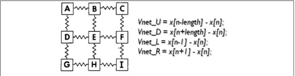
neighboring cells must be considered when calculating one cell’s potential, but 4 neighboring cells must be taken into account, as the cells are placed as in a matrix and no more along a line.

Figure 2.6: Scheme of connection between cells in the tissue model

Vm[m] = (x[n])+(step)∗((rad2∗ π (ρ ∗ Cm∗ deltx))∗(V net)− (Iion[n] + stim) Cm ); (2.7) where the following parameters are utilized:

• Vm[m] is the updated membrane potential of the cell whose position

in the voltage array is denoted by the index m (m=0,1...num cell). After having written into Vm the updated values for each cell, these

are copied into another array x, so that Vm is only a temporary vector;

• x is the state variable array, which contains the updated values of all the state variables. At the first time step, it is filled with the initial conditions, then the updated values of the state variables are copied from two temporary arrays into it. In particular voltage values occupy the first num cells positions of the array and n, like m, is an index which denotes the number of the cell (n=0,1...num cell). For each step, m and n denote the same cell, just in two different vectors and x[n] represents the value assumed by Vm[m] at the previous time

step;

• Vnet is the sum of the contributions in voltage deriving from the four