STATISTICAL METHODS FOR EXPLORATORY MULTIDIMENSIONAL DATA ANALYSIS ON TIME USE
Mary Fraire
1. EXPLORATORY AND CONFIRMATORY DATA ANALYSIS: TWO DIFFERENT APPROACHES FOR COMPLEX PHENOMENA
Until the 1950s, statistics’ principal meaning lay in direct and inverse inference. In the history of the two meanings of data analysis, confirmatory and exploratory, we can deduce that until the ’50s data analysis leant heavily in favour of confirma-tive analysis. Starting from the ’60s it was John W. Tukey (1962) with his writings and teaching who gave a decisive push in the opposite direction, by a series of important articles on the philosophical foundations of explorative analysis, and also putting forward ingenious methods that were widely welcomed and changed statistical activity. In his writings and teaching he found it useful to define what was meant by statistical data analysis, that is, the procedures for analysing data, the techniques for interpreting their results, the planning of methods for data col-lection and any computing and mathematical-statistical procedure that might be applied to data analysis. Statistics in the sense of drawing an inference from a sample and applying it to a population is therefore only a part of data analysis and not all of it (Morghenthaler, 2009).
Complexity is a cultural aspect of our knowledge: phenomena are what they are. In particular, in the empirical study of social phenomena it is important to underline that from the same phenomenon (e.g.. health, intelligence, quality of life, behaviour, opinions, but also employed and unemployed, GDP, etc.) it is possible to give different definitions from an operative point of view (that implies different measures and results of the measurement) because empirical language is not independent or, rather, it is ‘entangled’ with theory. There is a ‘gap’ between empirical concepts and measures that cannot be filled with single rules (Fraire, 1989). In this context, the exploratory approach of data analysis, in particular of exploratory multidimensional data analysis (henceforth EMDA) adapts very well to such complexity because, although the operative definition of phenomena in empirical observation is ‘relative’ to the observer-researcher, in the EMDA ap-proach it is necessary to render explicit the conceptual definition and formalise the problem to be analysed. In the matrices of the sets N of the statistical units
and K of the statistical characters, what has to be formed is a description that is pertinent (with regard to the problem to be analysed), satisfactory (complete, comprehensive) and homogeneous (in the unit of measurement in which the variables are expressed) thus allowing anyone to check the operative definitions adopted, the used/useable procedures as well as to clarify the interpretation of the results. (Lebart L. et al., 1997)
Although the two terms multivariate and multidimensional are often used as syno-nyms, there is a methodologically important distinction to be made between them that, all things considered, refers to the above-mentioned distinction between
con-firmatory analysis (verificative-predictive) and exploratory analysis (descriptive-reductive). Multivariate analysis regards the study of the relationships in a circumscribed
group of statistical variables, generally less than 10-15, studying their correlations and interactions generally of an order superior to two (e.g. analysis of regression, causal analysis, path analysis, structural equation models, etc.; log-linear models; ANOVA and MANOVA). (Corbetta, 1992). The principal aims of multivariate analyses are confirmative in the sense of validating hypotheses formulated a priori, or after an explorative analysis, on the set multivariate data, based on probabilistic models and statistical tests.
Multidimensional analysis of data includes three very numerous groups of
statisti-cal methods: classificatory (cluster analyses); factorial for two-way tables (princi-pal component analysis, simple and multiple correspondence analysis, multidi-mensional scaling etc.); analysis for multiple tables (three-way and multi-way data analyses). These are all analyses with a strong computational basis and therefore only possible with computers and the appropriate advanced software. Currently, the increased possibility of dealing with great masses of data through rapid com-plex calculations using hardware and software accessible to all and increasingly ‘friendly’ in their use has created the conditions for the wider diffusion and appli-cation of EMDA methods in the most diverse fields of research.
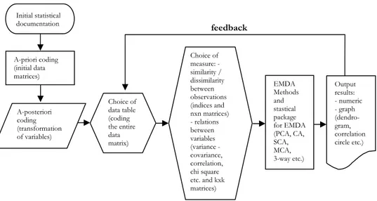
From a methodological and applicative point of view, beyond the specific EMDA methods that can be applied, it is useful to consider the exploratory analysis of data as a system composed of a number of equally important and inter-dependent phases. In each phase, choices have to be made that do not always have fixed rules or single criteria of choice and each having statistical and computerised aspects. It is possible to hypothesise 7 principal phases in which an EMDA is used, shown in the conceptual map in Figure 1 with special emphasis on the first four phases that make up the ‘preliminary phases’, the ‘crucial points’ of the en-tire process of data analysis (Fraire, 1994, 2006).
In Figure 1 the phases relate to the following aspects:
1st phase: initial statistical documentation: this is concerned with raw data, the
defini-tion of the object and the aim of the research, the plan for the material collecdefini-tion and gathering of data that can assume any form, whether paper (for example, compiled questionnaires) or in an IT format such as data files (in the form of da-tabases, worksheets, warehouses, etc.) or directly via web.
Figure 1 – Seven phases of EMDA.
2nd phase:regards a priori coding or the creation of the matrix of initial data, that
is, the transposition of all the raw data gathered in the 1st phase in the form of a matrix of ‘initial’ data. There are very many types of data matrices depending on the research situations and each has a given algebraic structure, a non-algebraic structure, or no structure (Fraire, 1995).
3rd phase: regards the a posteriori coding of the original data matrix as
transforma-tions of variables (categorical or cardinal) for different aims: for example, division into classes of the variables, transformations by ranks, transformations in dummy variables, fuzzy coding, arithmetic, algebraic and functional transformations, treatment of the missing values etc. This phase also contains the statistics (means, variability, correlations, asymmetry etc.) and graphs, especially IT, particularly adapted to the explorative analysis of the data (box plot, steam and leaf, Chernoff faces, etc.), for a first description of the data matrices.
4th phase: regards the choice of data table, on which to apply one (or more)
meth-ods of data analysis and requesting the coding of the entire data matrix selected (i.e. generalised contingency table, complete disjunctive table, Burt table etc.) or obtained as feedback from preceding data analyses carried out on the initial data matrix (e.g. the matrix factorial scoring in PCA, the ‘compromise’ matrix in 3-way analysis, etc.). In the multi-way analysis considered here this phase regards the choice (section 3.4) of one of the three possible research situations to which cor-respond three different types of coding as well as data tables (compromise matrix, trajectory matrix) obtained as ‘feedback’ from the execution of the three character-ising aspects of the 3-way data analysis employed here (sections 3.5, 3.6, 3.7).
The 3 successive phases regard:
5th phase: regards the choice of the measure: that is, the choice of a measure of
simi-larity/dissimilarity between units (ultrametric distances, distances, indices of dis-Initial statistical documentation A-priori coding (initial data matrices) A-posteriori coding (transformation of variables) Choice of data table (coding the entire data matrix) Choice of measure: - similarity / dissimilarity between observations (indices and nxn matrices) - relations between variables (variance - covariance, correlation, chi square etc. and kxk matrices) EMDA Methods and stastical package for EMDA (PCA, CA, SCA, MCA, 3-way etc.) Output results: - numeric - graph (dendro-gram, correlation circle etc.) feedback
tance, indices of similarity) or of a measure of relationship between characters (deviance-codeviance, variances-covariances, correlations, connections) adapted to the type of data table and to the chosen method of data analysis.
6th phase: regards the choice of the EMDA method and software.
7th phase:regards the output of the synthesis of the results: both numerical
(ei-genvalues, factorial weights, factorial scoring, trajectories etc.) and graphic (plots of factorial planes, circles of correlations, dendrograms, etc.).
In this work the use of EMDA will be proposed adapted to the data analysis on time use obtainable from the time-budget diaries of and surveys on time use, characterised by their large size, multipurpose nature and complex structure (sec-tion 2).
In particular two applications will be dealt with:
1) Analysis of the multiple tables using multi-way, in particular here 3-way data analy-sis, to analyse simultaneously a number of two-index data matrices on time use.
2) Global empirical models of time use. These analyses require the calculation of par-ticular tables and graphs based on cumulated frequencies, selected (intervals) time points, and categories of population engaged in all their daily activities. Such analyses are part of the sequential analyses on time use and time use for time points.
In describing the applications we will also refer to the conceptual map in Figure 1. Finally, it should be observed that the nature of data on time use often does not allow the respecting of the requirements imposed by the used/useable mod-els in multivariate analysis. For example with reference to modmod-els of regression:
– the assumption of normality of the residuals: despite the robustness of the model of linear regression, even using tobit regression the problem arises that the same set of independent variables can explain on the same plane the probability of the frequency of those who carry out the activity (doers) with the specific mean dura-tion of the activity itself. Deviadura-tions from the norm are found more often in daily diaries rather than in weekly diaries;
– the homoschedasticity of the residuals: many daily activities have a differentiated variability depending on the social groups under consideration, e.g. the variability in wages that depends greatly on age;
– the independence of the independent variables (incollinearity) and the inde-pendence of the residuals are often violated when a respondent has filled in more than one diary (e.g. for working days and holidays) or if there is more than one interviewee in the same family (K. Fisher, 2009).
2. THE SOCIAL NATURE OF TIME: TIME BUDGETS AND STUDIES INTO THE USE OF HUMAN TIME
From the point of view of statistics, time budget can be defined as follows: time budget is a continuous and analytical instrument of statistical observation (for populations or social groups), over limited periods of time (generally based on the
human circadian rhythm of 24 hours and the social relevance of said period: working day, holiday, day off etc.) of the way of using time on the part of a given collective. The ‘continuity’ of the observation requires special questionnaires (time-use diaries) that allow the recording of all the activities (under the form of a se-quence of ‘events’) carried out by the respondent during the period of observa-tion. The analyticity regards the following modalities of carrying out the activities of the collective under examination: the duration of each activity, the sequence in which it was effectively carried out on the day of the survey, its eventual
contempo-raneity with other activities, the place where it occurred, the persons present and/or
participating, as well as other eventual characteristics foreseen by the study (socio-demographic characteristics of the interviewee, characteristics of the day of the survey, enjoyment, satisfaction-dissatisfaction with the activities carried out and so on) (Fraire, 1986, 2004).
The dataset of time-budget studies are a complex structure. The methodologi-cal-statistical problems have to do with the difficulty of time-budget studies com-pared to the usual sociological studies that emerge from the consideration of time as a base unit of measurement both in the gathering as well as the elaboration of data. We will mention only some of the problems and point readers to more de-tailed expositions of these arguments in literature specific to the topic (Szalai, 1972; Istat, 1987; Fraire, 2004; Istat 2008). In the data survey phase: apposite ques-tionnaires should be provided with special reticulates (diaries) for the survey of times, the interviewees have to self-survey as regards the times taken for the activi-ties, the choice of the nomenclature of the daily activity often presents notable difficul-ties, and so on. In the data elaboration phase and if we wish to exploit all the tempo-ral modalities (cf. the definition of time budget) surveyable through time budgets (duration, frequency, sequence, contemporaneity, place, persons, subjective-perceptive aspects of the use of time) it is necessary to provide special codings both
‘a priori’ (1st phase of the EMDA), the creation of the matrix of the initial data: Time-Budget Data File, as well as ‘a posteriori’ (3rd and 4th phase) that are necessary for the automatic treatment of time-budget data because these have particular problems and solutions compared to traditional studies using questionnaires. We could mention, for example, in the coding of time-budget data the necessity for the ‘rectangularisation’ of the matrix of the initial data: the data files of the traditional studies of a social character are made up of rectangular matrices in the sense that each individual (line, record) has a fixed number of variables (columns, fields) and the content of each column is the same for all the interviewees. On the other hand, the time budget data file is made up of a matrix in which each subject (line,
record) has a different length due to the fact that each subject’s record has a
vari-able number of events (events: frequency of an activity) carried out in the 24 hours; the recording of the events occurs in the different orders in which they were carried out for each individual. Table 1 shows an example of the coding pat-tern at the level of the individual of time-budget data in which every record is therefore a string of events, E E1... j...E (each with 7 modality codes) rather than a k string of activities.
TABLE 1
Time-Use Data File: coding at the level of persons events characteristics background (1-st event) E1 ...
Ej ( j-th event) ... Ek (k-th event) persons Q1 Q2 ... Qk 1 2 3 4 5 6 7 1 2 . . . . . . . . . . . . . . . N
It is relevant to note that in the grid of time budget diaries (the special ques-tionnaire employed in the TUS) it is possible to fix the minimum length of each event (i.e. 10 minutes in the grid of ISTAT – Time-Use Survey) or leaving the re-spondent free: this choice will affect the computation of the temporal sequences of daily events also named ‘time-points data file’ from which come the ‘sequence time use’ tables and distributions.
One possible solution is therefore the ‘rectangularisation of the matrix of the initial data’ (3rd phase EMDA) through the coding for events instead of at the level of persons such as showed in a previous work of ours (Fraire, 1993).
At present in the industrially advanced countries new technologies in commu-nications and IT are accelerating the convergence of different ways of life (WoL) of different countries (being informed, working, caring for children, studying, looking after one’s health, shopping, social relationships and so on).
In this context, many countries reveal time-budget data that become increas-ingly relevant for several aims such as monitoring the similarities and differences and changes in the ways of life (WoL) of populations or given social groups, studying practical problems relating to social planning, e.g. linked to the use of the urban environment or relating to health (section 4).
Interest in the development of international comparative data on time use emerged at the end of 1980 with the Multinational Time Use Study (MTUS) whose scope was to gather the datasets from time use studies carried out in various nations and ren-der them comparable at international level. The ‘Multinational File’ that was called
World 1 in its first version is now (2009) up to the release of World 5.5 Version.1
1 The idea was to create a cross-nationally harmonized set of time-use surveys composed of
identically recoded variables. Harmonized version of the dataset is available for free downloading at the website: http://www.timeuse.org/mtus after registration. Dataset concerns 34 surveys for total population of N = 321.390 diarists and Xk=100 variables: X1-11 variables concerning country, day of
collecting data, type of diary (daily, weekly etc.) that follow X12-37 26 variables concerning
back-ground characteristics of the diarist and finally the activities performed (only primary activities) in two classifications: 41 activities and a more restricted set of 22 activities to cover surveys that have a more restricted set of activity codes.
In Italy, ISTAT in the field of the Multiscope Family Survey carried out the fol-lowing studies on Time Use on probabilistic samples: 1986-87 (n = 38,110 indi-viduals in 13,729 families); in 1996, a preparatory pilot study for the successive study on a few cases; 2002-03 (n = 55,773 individuals in 21,075 families) and 2009 ongoing (Romano, 2004). From a methodological point of view it is important we distinguish different but complementary aspects in time budget data analysis: 1) Transversal analysis on time budget: based on the duration of the activities (what)
and on the frequency of those who carried out the activity on the day being surveyed. 2Such durations can be Mg = generic mean durations referred to the
total of the population or social group under survey, irrespective of whether or not they carried out the activity on the day of the survey or Ms = mean specific duration referring only to carrying out the activity with an indication of the frequency of those who carried out the activity. The mean specific durations can also be referred to the primary or connected activities with the frequency of the couplings.
2) Sequential analysis of time use: the daily rhythm of the activities (when) based on the frequency of the population carrying out a given activity by time points (epi-sodes, intervals into which the 24 hours are subdivided); frequency of the population carrying out all the daily activities by time points (tables and
cumula-tive graphs of time use)3.
In the following paragraphs these two aspects, transversal and sequential, will be considered, applying two different statistical methods of exploratory multidi-mensional data analysis (EMDA).
3. TRANSVERSAL ANALYSIS OF TIME USE: MULTI-WAY DATA ANALYSIS
3.1 Multi-way data analysis: methods and software
Multi-way data analysis concerns the analysis of multiple tables. There are dif-ferent techniques of multi-way data analysis depending on the difdif-ferent study situations: Procrustean Analysis, Multidimensional Scaling metric and non-metric, Multiple
Factorial Analysis, Act-Méthode Statis and Act-Méthode Statis-Duale, Generalised Canoni-cal Analysis. In the field of multidimensional explorative and asymmetric data
analy-sis, multi-way data analyanaly-sis, and in particular three-way data analysis which will be employed here, constitutes a group of methods of great interest for the explor-ative, comparative and synthetic analysis of the multiple tables, that is, analysis in following different possible points of view of numbers of two-index matrices globally and contemporarily through a third ‘criterion’, ‘occasions’, chosen a pri-ori. The occasions can be times, places or any other criterion (qualitative or quan-titative). The aim of three-way analysis is that of comparing a number of studies,
2 It should be noted that with budget data it is also possible to analyse using the same
time-use indices: the places (where) in which one is found in the 24 hours irrespective of the activities carried out, and the persons (with whom) present and/or participating still irrespective of the activities carried out.
3 In this type of analysis too rather than activities we can also refer to the places or persons
research and inquiries when each of these has many variables observed in many statistical units.
In particular, in the following applications three-way data analysis will be consid-ered referring to quantitative data and, in particular, the Act-Méthode Statis and
Analyse Factorielle Multiple methods, employed using ACT-Statis and SPAD-Analyse des Tableaux Multiples: Statis and Analyse Factorielle Multiple software4.
3.2 Initial statistical documentation (1st phase EMDA): sources of data, sample, macro-units and activity-variables
Source of data: the source of the data employed for the applications is
repre-sented by a sub-file extracted from the dataset of the Time-Use Study 1988-895 of ISTAT. The time-use dataset employed had a dimension of 2437 bytes for every interviewee characterised by 173 variables of which: 23 variables on the socio-demographic characteristics of the interviewee and of the day of the survey, 150 variables relating to the activities (events): 3 50 (3 variables for every event) and considering a maximum of 50 daily events per person.
Sample : concerning N = 327 couples (99% married and 1% cohabiting)
equiva-lent to 654 partners in work days and N = 361 couples (722 partners) on Sunday in mononuclear families living in major urban conurbations (11 Italian cities: Turin, Milan, Venice, Genoa, Bologna, Florence, Rome, Naples, Bari, Palermo, Catania.)
N=22 statistical units in the applications are represented by macro-units,
catego-ries of population, in particular here ‘categocatego-ries of partners’ obtained through cross-ing the modalities of the followcross-ing variables of analysis and variables relatcross-ing to life cycle (classification variables) recorded in table 2.
TABLE 2
Analysis Variables and Life Cycle Variables for the set N = 22 macro-cases
ANALYSIS VARIABLES Value label
1. DAY Day of Interview:: Sunday ; Workdays (from monday to friday)
2. SEX Sex:Man; Female
3. PARTNER AGE Age Class: 15-24; 25-44; 45-64; 65-74; 75-84;85+ 4. AVERAGE AGE IN THE COUPLE Average Age Class: 20-35 ; 36-50 ; >50 5. EDUCATION Education level: High ;Middle; Low
6. EMPSTAT IN THE COUPLE (married/cohabiting) Employment Status in the couple:
Both employed; One only employed; None employed LIFE CYCLE VARIABLES Life cycle
7. CHILD <18 YEARS LIVING IN THE COUPLE Without children less 18 years living in the couple ; with children less 18 years living in the couple;
8. AGE OF YOUNGEST CHILD LIVING IN THE
COUPLE Youngest Age: Adult living with at least one child aged < 5 ; Adult living with at least one child aged 6-11; Adult living with at least one child aged 12-18 .
Source: M. Fraire, E. Koch-Weser Ammassari (1995, 1997)
4 The acronyms have the following meanings: ACT is for Analyses Conjointes des Tableaux; STATIS
indicates Structuration des Tableaux A Trois Indices de la Statistique; SPAD Système Portable pour l’Analyse
des Données. The two types of software mentioned are respectively from the Unité de Biométrie
(IN-RA-ENSA) of Montpellier, France and the CISIA, Centre International de Statististques et d’Infor- matique Appliquée, Montreuil Cedex, France.
5 In the following analyses there will also be a comparison with the data from ISTAT Time-Use
The 22 categories of partner were therefore the following (indicated with their labels): 1. Females; 2. FemaleNotEmployed; 3. Femployed; 4. FlowEducLev; 5. FhighEducLev; 6. FWithChild<18 years; 7. FWithouthChild<18years; 8. FMid-dleEducLev; 9. FWithYoungestChild<05years; 10. FwithYoungestChild; 11. FWithYoungestChild 12-18 years. The same for the 11 cases of male partners.
Xk (k = 1, 2, ..., 9) = 9 variables here are made up of 9 daily activity groups
that include all the activities carried and possessing the following characteristics: they are primary activities, that is, principal activities not carried out contemporar-ily with others or, in that case, considered primary anyway, the order of the activi-ties is conventional, and only for the data analysis of the following times (section 4) by convention the (primary) activities are ordered from non-obligatory activi-ties (free time) to those that are more obligatory (working, eating, sleeping); it should be noted that the choice of the classification of the activities with different possible levels of analyticity (digits)is carried out by the researcher on the basis of the study’s aims – here the 9 primary activity groups considered with the activities are the following: 1. TV (TVand video); 2. OMED (Other mass media (radio, music, reading); 3. FREE (Free time: leisure time (sports, outdoor activities, hob-bies and games unspecified); volunteer work and informal help to other house-holds; 4. SOCI (Socializing (participatory activities, social life and entertainment and culture).; 5. TRAV (Travel including travel for work); 6. H&FA (Home and family care); 7. WORK (gainful work, study); 8. EATS (Meals); 9. SLEEP.
3.3 Two- and three-index matrices (3rd phase of EMDA: a posteriori coding)
If P is the statistical or collective population defined by: ( 1, 2,..., ) ( 1, 2,..., ) j i N i n P x X j k (1)
in which i is the individual or statistical unit (s.u.) belonging to the total N: iN (i = 1, 2, ..., n); the total N is the total of all the n s.u. and is generally supposed to be finite and numerable (in socio-demographic types of study; N is, on the other hand, infinite in theoretical populations or in particular experimental studies), Xj is the statistical or variable character (table 3) of matrices of intensity or quantitative data, it is a variable belonging to the total X of the k statistical characters: XjX (j = 1, 2, ..., k); the total X is defined “a priori”. The statistical datum xij (i = 1, 2, ..., N; j = 1, 2,..., k) represents real numbers that can be:
– intensity (generic or specific mean durations of the time taken for each activity under consideration)
– relative frequencies (percentage of the member of the macro-unit considered that carried out the activity in the day under consideration); rational positive num-bers in a contingency matrix that in the case of 3-way analysis has to be normalised6.
6 Obtained examining the absolute frequencies in line with the numerousness N of the statistical
units (units of analysis) considered on each ‘occasion’ to bear in mind the diverse numerousness of the populations on each of the occasions considered.
The 2-way7 and two-indices matrix XN,K at n lines at k columns is reported in table 3:
TABLE 3
Two-indices quantitative matrix
11 12 1 1 21 22 2 2 , 1 2 1 2 ... ... ... ... ... ... ... ... ... ... . ... ... ... ... ... ... ... ... ... ... j k j k N K i i ij ik N N Nj Nk x x x x x x x x X x x x x x x x x
If we refer to the research situation considered here and to the transversal analyses of time use (section 2) what we are dealing with in particular is a matrix
intensity or quantitative data insofar as the abovementioned matrix Xn,k is com-posed of statistical data xij represented by real numbers,
– each line of the matrix can be seen as a numerical vector to k dimensions indi-cating the coordinates of a point-individual in a space Rk of k-dimensions, called space of the statistical units. In this application i-th row is the whole time-use profile
(description) of i-th individuals or category of individuals (partners). If the
row-sum is equal to 1440 minutes the row is i-th category’s time-budget (because
activ-ity duration is referred to all persons of the population’s category). Compari-sons among rows (also transforming data in % of the 24 hours = 100) give the differences in time-budgets of the 22 categories of population (partners). – each column of the matrix is represented by a numerical vector to n dimensions
indicating the coordinates of a point-individual in a space Rn of n-dimensions, called space of the variables. The j-th column is the distribution of average durations of j-th
activity among N = 22 categories of partners. Each column gives consistency (amount of time spent) and dispersion of j-th activity (primary activity group) among 22 categories considered.
– the statistical datum xij (i = 1, 2, ..., N; j = 1, 2, ..., k) = statistical data which can be
alphanumeric codes or real numbers.
In this application the data considered is average duration in minutes (and decimals) of the i-th whole category of population (including persons who had not performed the activity) for j-th primary activity. The choice of referring the activity’s average duration to the whole population or only to those who have performed the activity (‘doers’) is related to two different meanings and research interests: a) analysing the incidence of average duration of each activity in the 1440 minutes = 24 hours = 100 therefore focusing analysis on time-use ‘budget’; b) analysing the real, ‘typical’ duration of each activity, focusing analysis on time-use
structure.8
7 By mode what is intended is the type of information considered in the matrix under study; in
this case, for example, the “individuals” mode and “variables” mode, but they could also be modes such as places, times, judges, etc. The indices indicate, on the other hand, the criterion for classifica-tion of the “statistical datum” xij where iN (i = 1, 2, ..., n) are the individuals and XjX for j = 1,
2, ..., k are the statistical variables being considered.
As I note such matrices possess an algebraic structure of Euclidean vectorial space; this means that they can be subject to all the operations between matrices and the majority of the data analysis methods, whether predictive or explorative; further-more, such matrices can be subject to different metrics among s.u. (ultrametric dis-tances, Minkowski, Mahalanobis, etc.) or among variables (deviances and codevi-ances, variances and covaricodevi-ances, correlations, etc.).
Schematically, a 3-mode and 3-way matrix is indicated as follows: referring to the case under consideration, 3-mode and 3-way data analysis, that is, “cubic” data9, could be represented in the following way
,
OXN K in which O = occasions, N = statistical units or cases, K = variables.
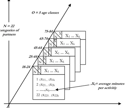
Two different hypotheses of ‘occasions’ particularly interesting for the EMDA time-use data are: age classes and countries. In this article we will refer to 3-way data analysis with the ACT-STATIS method, adapted to matrices of quantitative data and in particular to the example in Figure 2 in which the third criterion is ‘age classes’ while we refer to a previous work of ours (Fraire, 2006) for 3-way analysis in the case in which the third criterion is represented by the nations.
Figure 2 – Three-way time-use analysis when occasions are age classes.
contingency table. In 3-way analysis frequencies had to be normalized weighting the absolute fre-quency with N total population of each ‘occasion’.
9 Cubic data is structured as a multidimensional hypercube in which every side is a dimension; these
al-low even latent data to be analysed and modelled multidimensionally with an aim that is both pre-dictive and classificatory for the identification of typologies, models and data structure.
X1... Xk 1 1x11... 1x1k 2 1x21... 1x2k .. ...rxij... 22 1x221 . 1x22k X N X1... Xk 1 1x11... 1x1k 2 1x21... 1x2k .. ...rxij... 22 1x221 . 1x22k X N X1... Xk 1 1x11... 1x1k 2 1x21... 1x2k .. ...rxij... 22 1x221 . 1x22k X N X1... Xk 1 1x11... 1x1k 2 1x21... 1x2k .. ...rxij... 22 1x221 . 1x22k X N
K = 9 activity groups (exhaustives of all daily activities)
X1... Xk 11x11... 1x1k 21x21... 1x2k .. ...rxij... 221x221 . 1x22k X N N = 22 categories of partners 18-24 25-44 45-64 65-74 75-84 O = 5 age classes rXij= average minutes per activitiy
3.4 A posteriori coding of the 3-way data matrix: the choice of data table (4th phase of EMDA)
It is important to distinguish the type of 3-way data table that has to be con-structed (a posteriori coding corresponding to the 4th phase of EMDA) depend-ing on the research situations: 1) a matrix of dimension [N, (K O)] in which the
K variables are considered diverse found on O successive occasions and the N s.u equal.; 2) a matrix of dimension [(N O), K] in which the K variables are consid-
ered equal and the N s.u. diverse found on O successive occasions; 3) a matrix of dimen-sion [(N K), O] in which are considered equal both the N s.u. and the K variables found on O successive occasions.
In this work, the research situation considered is that described at point (3), that is, the K = 9 variables, primary activities, can be considered equal as can the N = 22 categories of partner on O occasions represented, in this case, by the 5 age classes. The 3-index data matrix under consideration can be indicated as:
( )
5 . workday 22 , 9 ( ),
O age classes X N partners K activities X N K O (2)
defined by the following elements:
Xj (j = 1, 2, ..., k) = 9 primary activities (table 4); N = 22 types of partners (table 2);
Or (r = 1, 2, ..., 5) = partners’ age classes: 18-24 years; 25-44 years; 45-64 years;
65-74 years; 75-84 years
rx (r = 1, ..., 5; i = 1, ..22; j = 1, ..., 9) = average duration (in minutes and ij
decimals) referred to all persons of i-th partner’s category in j-th activity in r-th occa-sion. I-th row is the time budget of i-th partner. Figure 2 reports the time use way data of the application. Table 5 reports a synthetic example of time use
three-way matrix coded in a suitable form for the situation research (application) under
consideration and the software employed.10
In particular, table 4 reports the data table that constitutes the 3-way data ma-trix, considered for the multi-way analyses that follow and referring in particular to the form requested, the ‘piling’ of the 5 matrices, using the statistical software ACT-STATIS.
10 With SPAD-méthode STATIS software this table would be built, rather, placing the matrices
of the occasions under consideration consecutively. All the analyses reported here of the inter-structure, intra-structure or compromised structures and trajectories were carried out using ACT-Méthode STATIS-CISIA software.
TABLE 4
The ‘a posteriori’ coded time-use three-indices matrix of the application
In which:
– the line vectors xi (i = 1, 2, ..., 22) are the time budgets (in minutes) expressed in generic mean durations for each category of partner for each of the daily ac-tivities (note that the total per line is equal to 1440 = 24 hour);
– the column vectors xj (j = 1, 2, ..., 9) represent the distribution of mean times
dedicated to each activity group by 22 types of partners;
– the xij data are the generic mean durations (section 2). The data refer to a
work-ing day.
Four different 3-way analyses have been carried out: on workdays and Sundays and on average durations referring both to all persons and to doers. We shall re-port here synthetically the results referring only to workdays and average durations for
all persons.
It should be observed that the method of 3-way analysis is composed of three different aspects that are carried out in succession:
1) analysis of the inter-structure;
2) analysis of the intra-structure or compromised structure; 3) analysis of the trajectories.
In the following paragraphs the principal results of the three aspects will be ex-amined.
3.5 Analysis of the inter-structure (5th-6th-7th phase of EMDA)
The analysis of the inter-structure concerns the analysis of the structure of the tables by means of global representation and the distance between them with the aim of comparing the five ‘studies’ (age classes) to verify which are similar (that have similar representations to the individuals) and which are different (Escoufier Y., 1980). In the case examined, what has to be evaluated is if the 22 types of partners in respect to the variables considered (9 activities; including all daily ac-tivities, their time budget) have through the 5 age classes under consideration a structure that is similar, near. This means verifying if and which are the partners who, in reality, for their class of age maintained homologous structures, that is, they did not undergo structural changes (of the homologous points) in their time budg-ets in a working day and in which there was a change.
The similarity or dissimilarity between the 5 data tables can be measured both by using a metric based on distances between statistical units (for example, Euclidean, Manhattan, and Mahalanobis distances, indices of distance such as ² and so on) as well as by distances between variances-covariances (V), correlations (R) according to the type of ‘a posteriori coding’ chosen for the 3-way matrix. In the application under consideration, the considered coding (of the third type cf. par. 3.4) requires distances between the coefficients of correlation (Pearson, Escoufier RV etc.), in particular the coefficient of correlation RV of Escoufier having value 0 if there is the maximum dissimilarity and value 1 if there is the maximum similarity between couples in the tables. Table 5 shows the matrix of the RV coefficients and Figure 4 the global representation of the 5 tables of data of the first factorial level (1+ 2 =39.44% + 26,21%= 65.65% of total variance) obtained, similar to what happens in ACP, from the diagonalisation of the RV matrix of coefficients of Escoufier (1980). The data is standardised (3rd phase EMDA: a posteriori coding) because despite having the same unit of measurement,
in minutes, both the statistical units and the variables had means and variability that were very different for each of the 9 daily activities considered) which means that on the first factorial plane reported in Figure 4 the origin of the axes (*== 0) and the mean matrix WD coincide.
TABLE 5
Distances matrix of correlation coefficients (range: 0 = max distance (dissimilarity), 1 = max similarity between pairs of tables)
18-24 25-44 45-64 65-74 75-84 18-24 1.000 25-44 0.357 1.000 45-64 0.150 0.378 1.000 65-74 0.057 0.091 0.332 1.000 75-84 0.084 0.112 0.169 0.626 1.000 Some main points about table 5:
– most similar pairs of time use tables are: 65-74 / 75-84 age classes (RV = 0.626); 45-64 / 25-44 age classes but with RV coefficient = 0.378;
– most dissimilar pairs of time use tables: 18-24 / 65-74 age classes (RV = 0.057; 18-24 / 75-84 age classes (RV = 0.084).
From the plot of the five time-use tables on the first principal plane in Figure 3 it is possible to see that the time-use table referring to partners of the 45-64 age class is near the mean (WD) and is dissimilar to the other time-use tables and the age classes over and under the mean matrix (WD).
Figure 3 – Plot of the five time-use tables on first factorial plane (65,65% of total variance).
Notes: WD is the mean (compromise) matrix and WD = 0 because data are standardised (mean = 0
and standard deviation = 1).
3.6 Inter-structure or compromise (mean) analysis (5th, 6th, 7th steps of EMDA)
In the conceptual map of the 7 phases of EMDA (cf. Fig. 1) this analysis cor-responds to the 1st feedback: from the 7th phase of EMDA= output= mean matrix
(compromise, WD) that becomes the data table (4th phase of EMDA) for the analysis of the intra-structure.
The scope of the analysis of the intra-structure is that of identifying the
mean-individual-points (compromise) and the mean-variable points through the 5 occasions.
In other words, which categories of partner have most greatly contributed to variability, through the age classes, on the time budgets of a working day. With this aim we have to identify the ‘type of mean-partner’ and the corresponding ‘mean profile of time budget’ (in substance the ‘barycentre’ of time used for the age classes under consideration and the types of partners) and to what extent and which are the classes of partner that move furthest away.
The ‘mean’ matrix (WD) is called ‘compromise matrix’; this represents the syn-thesis of all the matrices and is given by the weighted arithmetic mean of the matri-ces of similarity or distance N N among individuals, in the case under consid-eration, for example, they are:
18 24 S22,22 25 44; S22,22 45 64; S22,22 65 74; S22,22 75 84 22,22; S (3) corresponding to the original matrices expressed in deviations from the mean,
weighted with the corresponding eigenvectors to the first greatest eigenvector of the matrix
ij C C (4) being ( ) ij i j C tr S S (5)
Based on the first eigenvector the compromised matrix WD is ‘robust’ insofar as it is not very influenced by the small variations in the matrices of similar-ity.(Rizzi,1989). It is important to verify that in these multi-way analyses the quanti-ties selected ‘make sense’ in relation to the phenomenon under consideration: here the compromise matrix undoubtedly has a clear meaning of ‘mean time budget’, typical of the categories of partners considered, irrespective of their age. For the analysis of the intra-structure, the compromise WD matrix forms a diagonal which, in the case under consideration and limiting ourselves here to reporting only the first two factors (compromise axes), has the following eigenvectors:
1 + 2 =39.44% + 26,21%= 65.65%
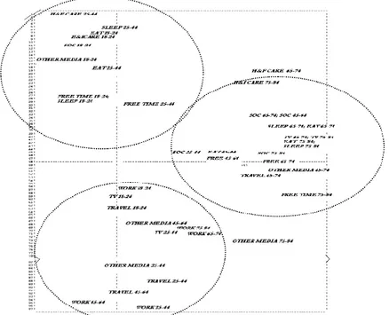
It is possible, therefore, to represent on the first factorial plain both the vari-ables (mean variable-points) and the s.u. (mean-individual-points) in respect of the first two compromise axes. Figure 4 limits itself here to reporting the plot of the mean variable-points (activity) in respect of the first two compromise axes. It can be noted that three types of partner can be clearly identified in respect to both the age classes as well as to the activities carried out (Figure 4) and that each cluster
Figure 4 – Plot of mean-variables (activities) points across five age classes on the first compromise
presents a greater incidence of particular activities between the 9 groups of activ-ity being considered. The clusters indicated schematically in Figure 5 are as fol-lows: cluster 1: adult (18-24/25-44) at home: sleep; socialising; eating; other media; free time; cluster 2: old (65-74/75-84) relaxation-routine at home: eat, sleep, travel, TV; cluster 3: adult (18-24/25-44) out of home: travel; work; other , the day con-sidered is a working day.
3.7 Analysis of the trajectories: comparing the 22 categories of partner in respect of their time
budgets through the five age classes
In the analysis of the trajectories we wish to compare the ‘trajectories’ of the 22 partners with regard to their time budgets through the 5 age classes with a view to identifying the role of each category of partner with respect to the differences in the use of time in a working day. In particular the analysis of the trajectories permits the comparison simultaneously and analytically of the individuals (22 partners) and the vari-ables (9 groups of primary activity including all daily activities) for the five age classes under consideration; that is identifying and comparing the ‘paths’ of each category of partner through the 5 age classes. To this end, it is possible to represent the trajecto-ries in many ways: representing each s.u. with respect to the factorial plains obtained from the analysis of the intra-structure (par.3.6) or reporting the trajectories of the s.u. with respect to the single factorial axes. Here we have chosen this last mode with reference only to the first factorial axis explaining the 42.48% of the total variance. In table 6 the factorial scores are of the 22 types of partner through the 5 age classes. It is also possible to show the 22 trajectories indexed showing on the vertical axis the
factorial scores referring to the first axis under consideration and on the horizontal the
five age classes under consideration.
TABLE 6
Trajectories of the 22 categories of partners across the five age classes. Factor scores on the first factorial axis (42,48% of the total variance)
Partners/Age classes 18-24 25-44 45-64 65-74 75-84 Male 0.0936 0.1546 0.1956 1.0745 1.1929 MNotEmploy * 0.4975 0.4339 0.6389 0.8231 Memploy 0.0936 0.1405 -0.1607 0.7379 * MLowEduc * 0.2492 0.4106 1.0625 1.1494 MMiddleEduc 0.0936 0.0905 -0.0347 1.0919 1.3140 MHighEduc * 0.1888 0.1256 1.1152 1.4180 MWithChild<18 0.0936 0.1561 -0.1527 * * MNoChild<18 0.1675 0.1485 0.501 * * MWithChild<05 0.0936 0.1429 -0.3478 * * MWithChild6-11 * 0.2146 0.0209 -1.2446 -0.8548 MWithChild12-18 * 0.0734 -0.1762 -1.2446 -0.8548 Female -0.2325 -0.2025 0.2607 0.6421 0.8231 FNotEmploy -0.2670 -0.1329 1.2403 0.9903 * FEmploy -0.1769 -0.0985 -0.8499 -1.2446 -0.8548 FLowEduc * -0.3785 0.2803 0.5953 0.8595 FMiddleEduc -0.2967 -0.2232 0.1978 0.9494 0.6611 FHighEduc -0.1825 -0.0961 0.3343 0.5866 -0.8548 FWithChild<18 -0.3480 -0.2597 -0.1268 * * FNoChild<18 -0.0455 0.1080 0.3860 0.6421 0.8231 FWithChild<05 -0.3480 -0.2991 -2.0525 * * FWithChild6-11 * -0.1510 * * * FWithChild12-18 * -0.2072 * * *
Commenting briefly on the results of the trajectories obtained Across five age
classes, it is possible to verify the change of position in time budgets of the same
category of partners with respect to the others. The most remarkable differences in time-budget trajectories, on a working day, among 22 categories of partners
across 5 age classes are the following: both male and female partners have similar
(among the same gender) time-budgets in age class 25-44 years but in increasing the age classes, 45-64 and above all 65-74, large differences in time-budget among different categories of partners of the same gender become apparent. In particular it is possible to know the category of partner (table 6): for example male high educational level with respect to male with youngest child < 6-11 and 12-18 years old living at home devote less time to work, TV, travel. It is useful to remark that 3-way data analysis confirms the large differences of time use by gender in the couple also when the third criteria, chosen ‘a priori’, is the partners’ age classes. 4. SEQUENTIAL ANALYSIS OF TIME USE
4.1 Meaning and aim of sequential analyses of time use
Having examined the transversal analysis of time use through 3-way analysis, we will now refer to the sequential analysis of time use.
Sequential analyses or analysis of the hourly sequences is based on frequencies, pre-arranged ‘time points’ (intervals, parts of hours, episodes) into which the 24 hours are subdivided (of a working day or a holiday) of those who carry out a given activity or who find themselves at those times in given places irrespective of the
activities being carried out, or who are, at those times, with given persons still irrespective of the activities being carried out.
Sequential analyses allow us to know the daily collective rhythm, the frequency by time points of the carrying out of the activity/activities or the use of places or of the types of people present and have particular importance in the analysis of the use of time for various reasons.
Knowing the hourly sequence of the activities with respect to the mean dura-tion of the activities allows us to know the diversity of the different social groups in the carrying out of the activities: even if a given activity has the same mean du-ration for two different collectives, for example, male professional work and fe-male professional work, it does not mean that said activity will be carried out in the same way on the day of survey. The hours when an activity is carried out re-count the lives of the individuals insofar as they are members of the society that has its own rules, calendars and daily habits. Time is a social construct that re-flects the rhythm of collective life. (Sorokin and Berger, 1939; Elias, 1986; Durk-heim, 1991).
In particular on the basis of sequential analysis it is possible to compare,
synthe-sise, and, construct empirical models of behaviour in the use of time both specifically
(re-ferring to a single activity or homogeneous group of activities) and global (refer-ring to all the daily activities).
Analyses by time points can provide cognitive elements that are useful for the resolution of practical problems such as those inherent to the urban environment and
the use of the city; problems connected to ecology and development of sustainable consump-tion such as knowledge of ‘rush hours’ and habits linked to particular social
con-sumptions (water, electricity, etc.), the rhythm of the carrying out of activities such as eating, sleeping, performing motor activities in relation to problems linked to health and lifestyle (insomnia, anorexia-bulimia, presence of chronic and degenerative illnesses, etc.).
For the sake of brevity and by way of an example, we will limit ourselves here only to analysing the global daily rhythm in the carrying out of all the activities of a working day, through the global empirical models on the use of time, leaving a complete vision of the different types of exploratory multidimensional analysis of sequential data to other publications (Fraire, 2007, 2008; ISTAT, 2007, 2008). 4.2 Empirical global models of time use: cumulative tables and graph on time use
All the daily activities carried out11 will be analysed with the frequencies with which they are carried out, pre-established time intervals, e.g. 144 intervals of 10 minutes each for different categories of population both working days and not. The choice of intervals of 5 or 10 minutes (or even less than 5 minutes, as was carried out in the International Comparative Inquiry on time budget carried out by UNESCO in 1966) is dictated by two motives: a) to obtain the real frequency of the activities, including those of a shorter duration; b) to have the greatest pos-sible analyticity of the intervals to provide continuity to the form of the distribu-tion as empirical models on time use. In this sense we speak of global empirical models of time use rather than specific empirical models, that refer instead to the frequency distribution by time points (intervals, episodes) for single activities. Such analyses require the tables of the cumulated relative percentage frequencies for the 144 time points and activity groups considered and the cumulative graphs of
time use.
Table 7 shows an example of a data table, a contingency matrix, N144;16 used choosing 144 time points, intervals of 10 minutes each, closed on the left and open on the right, in the 24 hours, e.g. 04:10 for 04:10 04:20; 04:20 for
04:20 04:30; up to 03:50 for 04:50 04:10 of the next day, and 16 primary
ac-tivities including all the daily acac-tivities.
In order to determine time intervals (“time-points” or episodes) into which to split the 24 hours, the maximum analyticity allowed by Istat data was selected (in diaries, the ‘minimum’ time unit was ten minutes): therefore, 144 time intervals of ten minutes, each one starting from the interval 4:00 4:10 , in table 7 indicated
with the “time-point” 4:10, 4:10 4:20, 4:20 and so on up to the last time interval
of 3:50 4:00 of the day after.
11 In this application activities have been classified in 16 subgroups including all the daily
TABLE 7
Percentage of total population (or social sub-groups) engaged in all daily activities collapsed in 16 subgroups at fixed time-points for the 24 hours (weekdays, Saturday, Sunday) being at given – Contingency matrix N144;16
Time -p oint s O ther pr ivat e acti viti es Ma ss -m ed ia Read in g Soci al r elat io n Sp or ts a cti vi tie s Ga mes a nd sport s acti viti es O ther le isure t ime acti viti es Parte ci pat ion in th e pu bli c li fe Fami ly -c are Hous eho ld act iviti es an d s hop pi ng Edu cati on an d train ing Prof es sio na l wor k C omu nic ati on Trav el f or ot her reaso n Eati ng (regular mea ls) Slee ping an d pers on al car e Tota l 04:10 0.0 0.1 0.2 0.1 0.0 0.0 0.0 0.0 0.1 0.0 0.0 0.4 0.0 0.1 0.0 99.0 100.0 04:20 0.0 0.1 0.2 0.1 0.0 0.0 0.0 0.0 0.1 0.0 0.0 0.4 0.0 0.1 0.0 99.0 100.0 04:30 0.0 0.1 0.2 0.0 0.0 0.0 0.0 0.0 0.0 0.0 0.0 0.4 0.0 0.3 0.0 99.0 100.0 ... ... ... ... ... ... ... ... ... ... ... ... ... ... ... ... ... ... 12:10 0.2 4.2 1.7 2.9 2.7 1.8 0.2 1.8 0.7 23.2 11.9 28.1 0.3 8.9 6.6 5.0 100.0 12:20 0.2 4.1 1.8 3.5 2.4 1.5 0.4 1.5 0.7 25.1 11.8 27.9 0.3 6.5 7.6 4.7 100.0 12:30 0.3 4.3 2.0 3.0 2.3 1.4 0.4 1.3 0.8 24.0 11.1 27.2 0.3 6.5 11.2 4.0 100.0 ... ... ... ... ... ... ... ... ... ... ... ... ... ... ... ... ... ... 16:50 0.2 6.0 2.0 8.4 6.2 4.5 0.6 2.9 2.8 13.7 6.5 22.8 0.3 9.4 1.9 11.9 100.0 17:00 0.2 6.0 2.0 9.2 6.5 4.2 0.8 2.9 2.6 13.0 6.7 22.7 0.3 9.8 1.6 11.6 100.0 17:10 0.1 6.8 1.8 9.4 7.4 4.1 0.7 2.5 2.6 13.1 5.6 20.2 0.3 13.6 2.2 9.5 100.0 ... ... ... ... ... ... ... ... ... ... ... ... ... ... ... ... ... ... 21:50 0.2 49.9 2.1 4.7 1.9 2.1 1.0 0.7 1.6 6.7 0.7 1.5 0.6 2.3 9.8 14.1 100.0 22:00 0.2 49.3 2.3 4.7 2.0 2.3 1.0 0.6 1.2 5.8 0.7 1.5 0.6 2.5 7.9 17.2 100.0 22:10 0.2 42.7 3.2 4.5 1.6 2.2 1.5 0.7 1.6 4.3 0.6 1.4 0.5 2.9 5.7 26.6 100.0 ... ... ... ... ... ... ... ... ... ... ... ... ... ... ... ... ... ... 03:50 0.1 0.2 0.2 0.2 0.0 0.0 0.0 0.0 0.0 0.0 0.0 0.2 0.0 0.4 0.1 98.6 100.0 04:00 0.1 0.2 0.1 0.1 0.0 0.0 0.0 0.0 0.0 0.0 0.0 0.3 0.0 0.4 0.1 98.7 100.0
Note that the order of the activities is conventional: generally the activity of sleeping is placed last in order to have, as we will see in the graphs that follow, this activity as a background for the cumulative graph on time use.
Starting from that, it is possible to construct cumulative graphs of time use that permit an extraordinary condensation of the huge quantity of information contained in the abovementioned tables and the possibility of being able to easily carry out the comparison.
By means of such analyses it is possible in fact to ‘contextualise’ each activity: with regard to the hours when they are carried out and therefore to its daily rhythm and with regard to the timetables and rhythms of all the others. The graphs in particular have in fact a triple reading that is described in the section below.12
4.3 The daily rhythm of partners’ activities in 2002-03 compared with the data from 1988-89 In particular, referring to a working day for married or cohabiting partners be-longing to mononuclear families and living in large urban conurbations, a com-parison will be carried out between the data from the Istat survey, Time Use in Italy carried out in 1988-89 (previously employed for the multi-way analyses de-scribed in par. 3) and in 2002-03. With this aim, a subfile of partners was created, analogous to that of 1988-89 (section 3.2), starting from the Istat 2002-03 data regarding mononuclear families with no isolated members; living in districts of
12 Cumulative graphs have been obtained from TABLE 8 (not cumulative percentages) by Excel
large urban conurbations (the same as in '88-89) + the outskirts of the metropoli-tan area13.
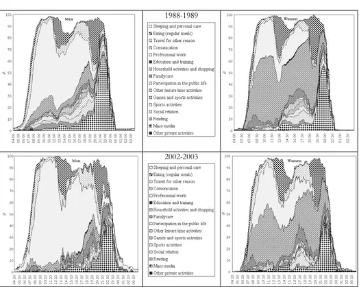
Figure 5 shows the cumulative graphs of time use referring for brevity only to the to-tal of the male and female partners, in a working day, on the basis of the 1988-89 and 2002-03 data.14 Before commenting briefly on the data, we refer to the possi-ble triple reading of the graph but it is to remark that for the possibility of being able to easily identify the activities the graph should to be in colours and here is not possible. We will limit ourselves here only to show an indicative example of the cumulative graphs in Figure 5 in which the activity names are listed in the same order for male and female and begin from the bottom to the top.
The background of the graph is the activity of sleeping, and generally (v. Fig. 5) we can note how both in the early hours of the morning (04:10 and following) as in the night-time hours (3:00 and following) it is practically 100% the frequency of those who are carrying out the activity of sleeping and no or almost no fre-quencies are marked for other activities.
Furthermore, the graph can be read three ways:
– a horizontal reading that allows both the frequency given by the width or nar-rowness of the band (each band has a colour that indicates a given primary ac-tivity) as well as its progress in 24 hours (form of distribution, modal hours etc.) to identify the rhythm of the activity, the time sequence in which it takes place in the day under consideration and for the category of population under consideration. It can also be noted that it is possible to identify the sequences of all the activities carried out and examine them comparatively for each time in-terval in the 24 hour.
– a vertical reading that allows us to know “at a given time of the day how many people are carrying out which activities” (distribution of cumulated frequencies between all the activities in a given interval). Since the frequencies are cumula-tive it is possible to know (by means of the difference between the extreme bottom of the frequency of the successive band and the extreme top of the preceding band) which is the frequency of a given activity in a given time band. – the contemporary horizontal and vertical reading that allows the examination of
the interdependence between the activities (e.g. some activities ‘occupy’ or ‘re-strict’ the space for others) and while this is not an analysis of causality it is still possible to know in which way the collective under consideration tends to or-ganize and ‘systemise’ its daily time.
13 Tables and graphs have been developed by Dr Elio Ascoli Marchetti - Codres (Cooperativa
Documentazione Ricerca Economica Sociale) in Rome.
14 The variables considered for mononuclear families were the following: Day of survey: weekday;
Sunday. Gender: M;F ; Average age of the couple: E2035; E3650; Eol50. Level of education: IstEl (university degree, second-class degree, high-school degree - 4-5 years); IstMd (high-school degree 2-3 years; grammar school); IstBa (elementary school, reading and writing, illiterate). working condition: EnOc (both work); UnOc (only one works); NsOc (neither of them work). cohabiting children: SenFg (wi-thout cohabiting children); ConFg (with minor cohabiting children). Age of the younger child: Fg05 (children aged between 0 and 5); Fg611 (children aged between 6 and 11); Fg1218 (children aged between 12 and 18). Overall, 30 types for weekdays and 30 for holidays, also considering total M and F.
1988-1989
2002-2003
Figure 5 – Workdays of partners by gender. Years 1988-1989 2002-2003 (cumulated frequencies in
percentage).
Commenting briefly on the results of the graphs the first thing to note is a general difference in the overall use of time between males and females, evident above all in the central part of the graph, which regards professional work and
do-mestic activities: the latter, as we would expect, are performed much more by
women than by men, while the opposite is true for professional work. The differ-ence does not reduce in a consistent way from 1988 to 2002-03 (it can be seen that this is the same even considering the ulterior variables of specification of the partners described in the note, e.g. when both are professionally employed). Re-ferring to the years ’88-’89 and ’02-’03 what has increased is the ‘complexity’ of the male and, above all, female day: in fact, for women the burden of domestic work and childcare does not decrease over the course of the 24 hours, but what in-creases in 2002-03 is the complexity of the working day, intended as the number of daily activities carried out; among these there are also those ‘for oneself’ that be-long in the realm of the personal. On the other hand we can note a generalised increase in nocturnal activity that in 1988-89 was limited only to male work, while in 2002-2003 they are varied and practised by the female population as well. The composition of these activities, though, is different between the two sexes. An-other significant difference present for both sexes is the diminution, in 2002-2003, of the use of the mass media in the evening hours in favour of their
gener-alised use throughout the day, and this can be explained by a wider ownership of personal computers and internet access, extensively used today not only in the workplace for work purposes.
CONCLUDING OBSERVATIONS
The applications of the exploratory multidimensional data analysis examined show they adapt very well to the dimensions and complex structure of the data with a view to exploring, comparing and synthesising said data, of drawing from them, despite their mass and maintaining the wealth of the complexity of infor-mation they provide, typologies, structures, interesting relations, and of discover-ing facts from them usdiscover-ing whatever procedure might serve the purpose. The only limits to such analyses are those imposed, other than by the statistical compatibil-ity of each technique with the nature of the data, by the creativcompatibil-ity of the re-searcher which is in turn linked to the knowledge of the phenomenon and the multidisciplinary approach that is indispensable for complex phenomena. In par-ticular:
– from the exploratory point of view they allowed the selecting of categories of populations and variables with the aim of constructing typologies, highlighting diverse data structures, constructing empirical models of time use that will also be useful for any eventual successive confirmatory analysis;
– from the comparative point of view what is evident is the great capacity for ana-lysing simultaneously numerous and complex cases (e.g., categories of popula-tion) and many variables (e.g.. in the analyses of time use, the number of activi-ties examined can also be very high)
– from the point of view of the synthesis the heuristic characteristics of the inter-pretation of the results of the classifications and factorisations provided by EMDA, typologies and underlying dimensions adapt well to the fuzzy nature of human behaviour.
Department of Social Research MARY FRAIRE
and Sociological Methodology “Gianni Statera” University of Rome – La Sapienza
REFERENCES
ACT-STATIS, (1989), Analyse conjointe de tableaux quantitatifs, Méthode STATIS, CISIA, Saint
Mandé (France).
S. BOLASCO, (1999), Analisi Multidimensionale dei dati, Carocci Ed., Roma.
P.G. CORBETTA, (1992), Metodi di Analisi Multivariata per le Scienze Sociali, il Mulino, Bologna. É. DURKHEIM, (1991), Les formes élémentaires de la vie religieuse, Puf, Paris.
N. ELIAS, (1986), Saggio sul tempo, Il Mulino, Bologna.
B. ESCOFIER, J. PAGÈS, (1984), L’analyse factorielle multiple, in Cahiers du Bureau Univ.
Y. ESCOUFIER, (1980), L’analyse conjointe de plusieurs matrices, in Biométrie et Temps, Jolivet et
al. (eds.), Société Francaise de Biométrie, Paris.
K. FISHER, (2009), The analysis of time-use data, in the web site: http://www.timeuse.org/mtus
on line M-TUS Documentation (World 5.5 Version), Chapter 5.
M. FRAIRE, (1986), I Bilanci del Tempo, in B.Grazia-Resi, Problemi di Statistica Sociale, Ed.
La Goliardica, Roma.
M. FRAIRE, (1989), Problemi e metodologie statistiche di misurazione di fenomeni complessi tramite
indi-catori e indici sintetici, in Statistica, anno XLIX n. 2.
M. FRAIRE, (1993), Coding Approaches, Tables and Graphs on Time Budget Data Towards Identifying
Temporal Sequences of Daily Events, ISTAT, NOTE E RELAZIONI N. 3.
M. FRAIRE, (1994), Metodi di Analisi Multidimensionale dei Dati. Aspetti statistici e applicazioni
in-formatiche, CISU, Roma.
M. FRAIRE, (1995), Multidimensional data analysis and its preliminary phases: statistical aspects, in
Rizzi A. Ed., Some Relations Between Matrices and Structures of Multidimensional Data Analysis, Applied Mathematics Monographs, n.8, Giardini Editori e Stampatori, Pisa, pp. 5-51.
M. FRAIRE, KOCH-WESER AMMASSARI E., (1995), Televisione e tempi familiari, Sociologia del lavoro,
n. 58.
M. FRAIRE, KOCH-WESER AMMASSARI E. (1997), Lo sport nel contesto e nei ritmi della vita quotidiana, in MUSSINO A. (a cura di), Statistica e Sport: non solo numeri, Società Stampa Sportiva, Roma.
M. FRAIRE, (2004), I Bilanci del Tempo e le Indagini sull’Uso del Tempo. Metodologie di rilevazione e
analisi statistica dei dati sull’uso del tempo umano giornaliero, Ed.CISU, Roma.
M. FRAIRE, (2006), Multi-way Data Analysis for comparing time use in different countries. Application
to time-budgets at different stages of life in six european countries, in eIJTUR (Electronic Journal
of Time Use Research), Univ.of Lueneburg (Germany) in Vol. 3, N. 1.
M. FRAIRE, (2007), Analisi delle sequenze orarie delle attività e dei contesti spaziale e sociale nei grandi
centri urbani. Applicazioni alla differenza di genere, in ISTAT, AA.VV., I tempi della vita
quotidiana, Argomenti n. 32, (anche on line).
M. FRAIRE, (2008), Time Sequence Analysis of Activities as well as Space and Social Context in Large
Urban Centres, in ISTAT, AA.VV., Time Use in Daily Life. A Multidisciplinary
Ap-proach to the Time Uses’s Analysis, op. cit.
ISTAT, (1987), L’uso del tempo in Italia – Indagine Multiscopo sulle famiglie 1987-1991, vol. 4. ISTAT, (2007), I tempi della vita quotidiana, Argomenti n. 32 (anche on line).
ISTAT, (2007), Uso Tempo 2002-03, collana Informazioni n. 8.
ISTAT, (2008), AA.VV., Time Use in Daily Life. A Multidisciplinary Approach to the Time Uses’s
Analysis, Argomenti n. 35 (on line).
L. LEBART, A. MORINEAU, M. PIRON, (1997), Statistique Exploratoire Multidimensionnelle, Dunod, Paris. S. MORGHENTHALER, (2009), Exploratory Data Analysis, Jhon Wiley & Sons, WIRES
Comp-stat, 1-33.
A. RIZZI, (1989), Analisi dei Dati. Applicazioni dell’informatica alla Statistica, NIS, Roma. M.C. ROMANO, (2004), Le indagini multiscopo dell’Istat sull’Uso del Tempo in FRAIRE M., I Bilanci
del Tempo e le Indagini sull’Uso del Tempo. Metodologie di rilevazione e analisi stati- stica dei dati sull’uso del tempo umano, op. cit.
P.A. SOROKIN, C.Q. BERGER, (1939), Time Budget of Human Behavior, Harvard University Press,
Cambridge.
A. SZALAI, (1972), The Use of Time, Mouton, Paris.
J.W. TUKEY, (1962), The future of data analysis, Annal Math Stat, 33: 1-67.
SUMMARY
Statistical methods for exploratory multidimensional data analysis on time use
After a brief introduction on the different approaches between exploratory multidi-mensional data analysis (EMDA) and confirmatory multivariate data analysis (CMDA) the paper deals with EMDA and in particular multi-way methods suitable for comparing sta-tistical studies when each of them has many variables observed on many cases as in time use data analysis. Then the paper focuses on the two main time-use analyses: transversal and sequential analysis using respectively 3-way data analysis and time-points cumulative
frequencies tables and graphs.Application concerns differences in time use of categories