View of Determinants of the Italian labor productivity: a quantile regression approach

(1)

DETERMINANTS OF THE ITALIAN LABOR PRODUCTIVITY: A QUANTILE REGRESSION APPROACH

M. Velucchi, A. Viviani

1. INTRODUCTION

Since the early ’90s, the Italian economy, like several other countries all around the world, has been characterized by a relative decline in economic growth rates. The economic literature widely discusses the roots of this feature of the Italian productive system: low labor productivity, small firm size and/or high specializa-tion in tradispecializa-tional, low-tech sectors.

This paper deals with the heterogeneous performance of Italian firms’ labor productivity and investigates how some firms’ characteristics seem to affect the dy-namics of the Italian firms’ labor productivity in recent years (1998-2004). To this aim we use an original panel recently developed by the Italian National Institute of Statistics at a micro level (firm level). We estimate a non linear production function and a quantile regression approach. We test how a set of firms’ characteristics may influence the poor performance of Italian firms labor productivity growth in the period considered. We run models on manufacturing and focus on three of the most internationalized sectors in Italy (food, textiles and mechanical machinery).

The original database and the quantile regression allow us to highlight that la-bor productivity is very heterogeneous and that the relationships between lala-bor productivity and firms characteristics (like innovation, investments, internation-alization mode) do not hold uniformly across quantiles. We disentangle the effect of a set of variables on different levels of labor productivity showing that what is relevant for highly productive firms may not work for low productive firms. Thus, using the quantile regression approach we show that the medium estimates obtained with GLS do not capture the complex dynamics and heterogeneity of the Italian firms labor productivity. Innovativeness and human capital, in particu-lar, have a larger impact on fostering labor productivity of low productive firms than that of high productive firms. In general, we find evidence of a strong posi-tive relationship between labor productivity growth and internationalization of firms, investments in intangible assets and innovation.

The paper is structured as follows. In section 2 we briefly revise the literature on labor productivity, in section 3 we present the original database by the Italian National Institute of Statistics, in section 4 we illustrate how to adapt a quantile

(2)

regression approach to a labor productivity empirical analysis and in section 5 we discuss the results. Section 6 briefly concludes.

2. THE LITERATURE

2.1 The debate on measures of productivity

Productivity is generally defined as the measure of output from a production process, per unit of input. Despite this simple definition, the debate about inputs and output and how to combine them, i.e. the debate on different measures of productivity, has grown dramatically during the most recent years. Of course, dif-ferent types of input measure give rise to difdif-ferent productivity measures. For ex-ample, labor productivity measures involve dividing total output by some meas-ure that reflects the amount of labor used during the production process. The tal number of work hours is a possible input, although several studies use the to-tal number of workers employed but the relative index changes accordingly. La-bor productivity is a partial productivity measure because it only considers one input-labor. Among other partial measures we may include: output per unit of capital, or output per unit of intermediate materials consumed in the production process, or output per unit of energy consumed. Multifactor productivity meas-ures, sometimes referred to as total factor productivity measmeas-ures, instead, com-bine several of these partial productivity measures into a more comprehensive, inclusive measure that captures how much output is produced relative to a bundle of several inputs, where the latter is calculated as a weighted sum of many inputs.

Four main approaches can be drawn to describe productivity measures: the growth accounting approach, the index number approach, the distance function approach and the econometric approach (OECD, 2001). Growth accounting en-ables output growth to be decomposed into the growth of different inputs (typi-cally capital and labor) and changes in total factor productivity. This approach re-quires the specification of a production function, defining the level of output produced at some particular time, given the availability of a given level of differ-ent inputs and total factor productivity (Barro, 1999; Proietti and Musso, 2007). The second approach mentioned is used by the vast majority of statistical agen-cies that produce regular productivity statistics. For example, the US Bureau of Labor Statistics and, among others, the Australian Bureau of Statistics calculate market sector multifactor productivity using the index number approach based on a Törnqvist index. The index number approach to calculate productivity in-volves dividing an output quantity index by an input quantity index to give a pro-ductivity index (Caves et al., 1982a, 1982b). The distance function based ap-proach to measuring productivity aims at separating it into two components using an output distance function that measures the distance of an economy from its production function. In principle, this technique enables a change in productivity to be decomposed into changes resulting from a movement towards the produc-tion frontier and shifts in the frontier. The output distance funcproduc-tion measures

(3)

how close a particular level of output is to the maximum attainable level of out-put that could be obtained from the same level of inout-puts if production is techni-cally efficient (Coelli et al., 1998 and Balk, 1998). In other words, it represents how close a particular output vector is to the production frontier given a particu-lar input vector. The econometric approach to productivity measurement con-cerns the estimation of the parameters of a specified production function (or cost, revenue, or profit function, etc). One advantage of the econometric ap-proach is the ability to gain information on the full representation of the specified production function. In addition to estimates for productivity, information is also gained on other parameters of the production function and this is not allowed us-ing the growth accountus-ing or index number approaches. Moreover, because the econometric approach is based on using information on outputs and inputs, there is greater flexibility in specifying the production function. Within the econometric framework it is also possible to test the validity of assumptions that underpin the growth accounting and index number approaches because of the sampling prop-erties of the production technology. However, Hulten (2001) has pointed out that the econometric approach to productivity measurement should be viewed as complimentary to the growth accounting and index number approaches.

2.2 The role of productivity on growth

Independently of the measure used, the economic literature generally agrees in saying that the long run economic growth of nations is ultimately determined by productivity growth. Indeed, in the long run, more productive workers experi-ence higher living standards because increased efficiency leaves space for larger income and more leisure time. For example, in a millennium perspective, Galor (2005) points out that productivity growth ended the epoch of Malthusian stagna-tion in the 1700s and was the root for sustained economic growth and industriali-zation of western economies. Productivity is generally acknowledged as the source of the unprecedented rise in human welfare in the past century, when liv-ing standards increased six-fold in the US, Italy and Germany, among others. However, productivity increases have not been constant over time. In the U.S. in the 70s, for instance, there has been a decline in productivity growth to about two-thirds of its pace of the last fifty years. Starting mid 90s, however, the U.S. productivity growth accelerated again and unemployment fell to levels not seen since the 1960s (Eicher and Strobel, 2008).

In particular, recent literature shows an impressive increase in studies on produc-tivity that use longitudinal micro-level datasets, focusing on plants or firms over time. The popularity of this emerging research can be found, in part, to increased availability of level data and to the development of a rich theoretical micro-economic foundation. But the most important stimulus has come from the fact that interesting questions about productivity and its effects on the economies behavior that can be addressed effectively only with microdata. Several country-specific cases have studied how recessions, changes in labour legislation, decentralisation of wage bargaining and increase in labour relations flexibility have affected countries growth

(4)

in recent years. A strand of the empirical literature discusses whether these factors have helped or hurt wage growth and employment growth (Hall et al., 2009) but doesn’t offer a unique interpretation to that question.

In Italy, for instance, what it seems to be evident is the subsequent crisis in la-bor productivity growth (Grassini and Marliani, 2009; Ferrante and Freo, 2011). There’s no agreement on the reasons behind this phenomenon, only a wide de-bate on the fact that the Italian specialization in low-tech, traditional sectors with low levels of investments in R&D and intangible capital favors the downturn trend in the labor productivity and economic growth of this country. On the con-trary, R&D activities, especially in high-tech sectors, large firms size, along with investment in equipment, seem to enhance the likelihood of having both process and product innovations. Both these kinds of innovation have a positive impact on firm’s productivity, especially process innovation (Griffith et al., 2004).

Another strand of literature suggests that internationalization of firms plays a role in increasing the labor productivity and firms’ performance in a country (Grif-fith et al. 2004; Arnold and Hussinger, 2005; Fryges and Wagner, 2008; Hansen, 2010). In particular, this literature emphasizes that firms involved in international activities through export or foreign direct investments are “different” from purely domestic firms in several respect (productivity, wages, skill intensity, see for all Mayer and Ottaviano, 2008). Following this perspective, there are relatively few firms ‘fit’ to compete in international markets and these firms are more productive, pay higher wages, employ more skilled workers, invest more in R&D. Melitz (2003), for instance, shows that there is a clear ranking between firms with different in-volvement in international markets: exporters are more productive than domestic firms, foreign investors more productive than exporters. Several authors focus on the performance of Italian firms during the recent years; they find mixed evidence and show that it is widely jeopardized across sectors, levels of technology and in-ternationalization mode (Castellani and Giovannetti, 2010; Dosi et al. 2010) 3. THE DATABASEISTAT

During the last decade, the interest of statisticians and applied economists has moved from macro to micro data, focusing on firms level data and a flourishing number of longitudinal databases at a firm level has been developed by several institutions (see, for instance, AIDA and AMADEUS by Bureau Van Dijk or the Survey on Entrepreneurship by Eurostat). During the last few years, also the Ital-ian National Institute of Statistics (ISTAT) has promoted large efforts to build affordable data on the Italian business activity and carried out business surveys at different points in time using different samples for several surveys or using dif-ferent samples and sources over time. However, only recently, ISTAT has pro-posed a panel (cross-sectional and time series perspective) on microdata at a firm level for Italy. This panel, which is used in this paper, is developed by the Italian National Institute of Statistics (Nardecchia et al., 2010) and contains information for the period 1998-2004. It is a catch-up prospective database: a cross-sectional

(5)

dataset from an archival source at some time in the past (in this case, 1998) is de-tected and then the units of analysis in the present by subsequent observation are added year by year. The catch-up panel is a particularly attractive design when we manage to isolate a source of baseline archival data which is especially rich in in-formation. On this basis, the panel has drawn all links between answering firms in 1998 survey with 2004 survey respondents. Detailed criteria are defined in order to take business transformation into account. Balance-sheet data are integrated but new firms, entering the market after 1998, are not included (for a detailed de-scription of the criteria used, see Nardecchia et al, 2010). This panel makes it pos-sible the analysis of firms’ behavior over time and/or grouping firms according to classifications chosen by the researcher (for instance gazelles, best performers or by economic activity, size or geographical area). The target population is repre-sented by firms with more than 20 workers.

The panel is mainly based on cross-sectional enterprises surveys microdata with the integration of administrative microdata for ensuring the matching of items over time and of eventual non-respondents. The cross-section enterprises surveys that characterize the panel show a widespread overlap time by time and a relevant longitudinal component. Four different sources are included. The first source is the census of Italian firms, the second is the so-called SCI survey, focusing on all firms with more than 20 employees, the third one is the so-called PMI survey that covers the firms with employment in the range 20-100 and the last one is the annual reports of incorporated firms collected by the Central Balance-Sheet Data Office of Italy. To avoid the risk of attrition and selection bias, the time span has been kept quite short and the panel cannot be used to analyze entry and exit dynamics of firms. Business transformation like mergers and acquisitions have been considered in the panel following a back-ward perspective (Biffignardi and Zeli, 2010).

The panel contains firms’ microdata on 13,573 units classified by sector of ac-tivity (ATECO 2002) for the period 1998-2004.

4. THE MODEL: A QUANTILE REGRESSION APPROACH

The prediction from most regression models – multiple regression, neural net-works, trees, etc. – is a point estimate of the conditional mean of a response (i.e., quantity being predicted), given a set of predictors. However, the conditional mean measures only the “center” of the conditional distribution of the response. A more complete summary of the conditional distribution is provided by its quantiles. The 0.5 quantile (i.e., the median) may serve as a measure of the center, and the 0.9 quantile marks the value of the response below which resides 90 quantile and the 0.05 quantile serves as the 0.05th, thereby conveying uncertainty. Quantiles arise naturally in social sciences. For example, one may desire to know the lowest level (e.g., 0.1 quantile) of income distribution, given the level of un-employment in a country; or the highest level of physical investment in the ma-chinery sector (e.g., the 0.9 quantile), given GDP growth of the last year. Recent

(6)

advances in computing allow the development of regression models for predict-ing a given quantile of the conditional distribution, both parametrically and non-parametrically. The general approach is called quantile regression, but the meth-odology (of conditional quantile estimation) applies to any statistical model (Koenker and Hallock, 2001). In linear regression, the regression coefficient represents the change in the response variable produced by a one unit change in the predictor variable associated with that coefficient. The quantile regression pa-rameter estimates the change in a specified quantile of the response variable pro-duced by a one unit change in the predictor variable. This allows comparing how some percentiles of the dependent variable may be more affected by certain pdictors than other percentiles. This is reflected in the change in the size of the re-gression coefficient. Standard errors and confidence limits for the quantile regres-sion coefficient estimates can be obtained with asymptotic and bootstrapping methods. Both methods provide robust results (Koenker and Hallock 2001), with the bootstrap method preferred as more practical (Hao and Naiman, 2007).

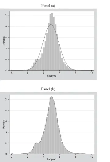
In our case, estimation of linearized models by quantile regression may be preferable to the usual regression methods for a number of reasons. First of all, we know that the standard least-squares assumption of normally distributed er-rors does not hold for our database because productivity has not a Gaussian dis-tribution (see Figure 1 below).

Whilst the optimal properties of standard regression estimators are not robust to little departures from normality, quantile regression estimates are robust to outliers and heavy-tailed distributions. The quantile regression estimator ˆ is invariant to outliers of the dependent variable that tend to infinity (Buchinsky, 1994). While OLS regressions focus on the mean, quantile regressions are able to describe the entire conditional distribution of the dependent variable. In the context of this study, high/low labor productivity firms are of interest and we wouldn’t dismiss them as outliers; on the contrary we think it would be very interesting to study them in some detail. This can be done by calculating coefficient estimates at various quantiles of the labor productivity conditional distribution. Finally, a quantile regression ap-proach avoids the restrictive assumption that the error terms are identically distrib-uted at all points of the conditional distribution. Relaxing this assumption allows us to acknowledge firms’ heterogeneity and consider the possibility that estimated slope parameters vary at different quantiles of the conditional distribution.

In a longitudinal context, GLS estimates have low efficiency in case of highly skewed data because these models use the mean as the measure of centrality. But what is more important in a practical situation is that it is more difficult to inter-pret what the mean measures when the data is skewed. In contrast to this the median (and quantiles in general), besides having higher efficiency than the mean for skewed data (Koenker and Bassett, 1978), always has an easy interpretation. Since it is common with skewed data in practical situations, and one does not know the distribution of the underlying population, this makes the quantiles a preferable approach to use, and motivates the use of quantiles regression for lon-gitudinal data, instead of the mean regressions.

(7)

Panel (a) 0 2 4 6 8 10 Pe rce n t 0 2 4 6 8 10 llabprod Panel (b) 0 2 4 6 8 10 Pe rc en t 0 2 4 6 8 10 llabprod

Figure 1 – Histogram and Normal Density Plot (Panel a) and Kernel Density Plot (Panel b) of Labor Productivity (in logs).1

The quantile regression model, first introduced in Koenker and Bassett’s (1978) seminal paper, can be written as

it it it

y x u

with Quant y x( it| it)xit 

where y is the dependent variable, x is a vector of regressors, β is the vector of parameters to be estimated, and u is a vector of residuals. Quant y x( it| it) denotes the θ-th conditional quantile of y given x. The θ-th regression quantile,

0 < θ < 1, solves the following problem:

(8)

' ' _:1 , : , : 1 1 (1 ) min min it it it it n it it it it it i i t y x i t y x y x y x u n n    _ _  _ _        _ _ _ _ _ _ _     







Where ( )  , which is known as the ‘check function’, is defined as 0 ( ) ( 1) 0 it it it it it u if u u u if u              _ _ 

which is then solved by linear programming methods. As θ increases from 0 to 1, we can trace the entire conditional distribution of y, conditional on x (Buchinsky, 1998). More on quantile regression techniques can be found in the surveys by Buchinsky (1998) and Koenker and Hallock (2001).

As most of the literature assume, we estimate the following non linear Cobb-Douglas production function in a reduced form (in logs):

2

1 1 2 3 4 1

54 1 6 7

8 9

log( ) log( ) ( _ ) ( _ ) log( _ )

log( ) log( _ ) log( _ )

log(exp_ ) log(exp_ )

it it it it

i t it it

it it t it

labprod k ratio wtob ratio wtob inv rd

patents imp eu imp extraeu

eu extraeu                            

Where labprod is the proxy for labor productivity (sales per worker for each firm i at time t), k is the level of physical capital invested per worker by firm i at time t-1, ratio_wtob is a proxy for the human capital investment of firm i at time t (the ratio of white to blue collars number). Then we add two proxies for invest-ments in intangible capital: inv_rd are the expenditures in research and develop-ment activities of firm i at time t-1 and patents that are the number of patents reg-istered by firm i at time t-1. We also include a set of predetermined variables that control for the internationalization mode of firm i at time t: imp_eu and exp_eu are the share of sales imported and exported (respectively) from/to European coun-tries while imp_extraeu and exp_extraeu are the share of sales imported and ex-ported (respectively) from/to countries outside Europe. We also control for common macroeconomic shocks by including year dummies (_t).

5. THE RESULTS

5.1 Descriptive Statistics

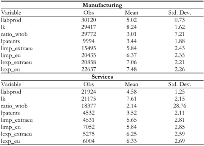
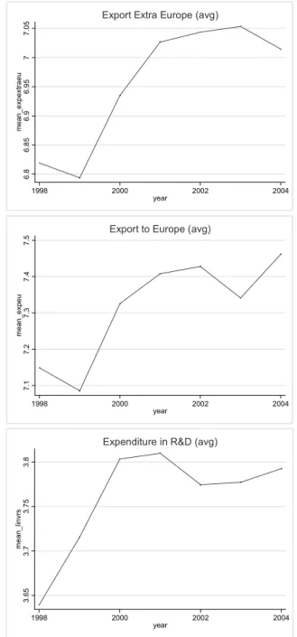
Table 1 reports descriptive statistics for selected variables in manufacturing and service sectors, Table 2 reports the same descriptive statistics disaggregated on labor productivity quantiles and Figure 2 shows the dynamic dimension of the panel. We show, for instance, that during the period considered (1998-2004) the Italian economy has experienced an increase in the average labor productivity, in-vestments in physical capital, openness to trade as well as an increase in average expenditure in R&D and innovativeness while the human capital proxy shows a

(9)

peak in 2001 and then reverts towards 3%. The 2001 crisis is not evident but we notice a slowdown slightly before, in 1999-2000. Table 3 focuses on those of in-ternationalized firms. According to the literature, this very preliminary analysis shows that internationalized firms are more productive and invest more both in physical and human capital (Mayer and Ottaviano, 2008). The innovativeness proxy (patents registered per year) seems to be quite homogeneous across manu-facturing and service sectors, while internationalized firms have a slightly higher average level of innovativeness and expenditure in R&D.

Table 4 reports descriptive statistics on the manufacturing sectors that best represent Italy in the international scene: food, textiles and mechanical machinery (Italian Institute for Foreign Trade, 2010). These sectors represent the Italian specialization in traditional, low tech and high quality sectors, with low levels of investments in R&D and human capital, the so called “Made in Italy” sectors.

TABLE 1

Descriptive Statistics for Manufacturing and Services

Manufacturing

Variable Obs Mean Std. Dev.

llabprod 30120 5.02 0.73 lk 29417 8.24 1.62 ratio_wtob 29772 3.01 7.21 lpatents 9994 3.44 1.88 limp_extraeu 15495 5.84 2.43 limp_eu 20435 6.37 2.35 lexp_extraeu 20838 7.06 2.21 lexp_eu 22637 7.48 2.26 Services

Variable Obs Mean Std. Dev.

llabprod 21924 4.58 1.25 lk 21175 7.61 2.15 ratio_wtob 18377 2.14 28.76 lpatents 4532 3.52 2.11 limp_extraeu 4531 5.65 2.81 limp_eu 7052 5.84 2.85 lexp_extraeu 5275 6.25 2.59 lexp_eu 6004 6.33 2.69 TABLE 2

Descriptive Statistics for Manufacturing by labor productivity quantiles

Quantiles 1% 5% 10% 25% 50% 75% 90% 95% Variables llabprod mean 1.54 3.03 3.54 4.36 4.96 5.49 6.00 6.35 st. dev. 0.90 0.03 0.03 0.01 0.01 0.01 0.02 0.03 Lk mean 6.47 6.17 6.63 7.44 8.42 8.64 9.23 9.34 st. dev. 2.18 2.02 1.38 1.27 1.48 1.61 1.70 1.46 ratio_wtob mean 0.48 0.39 0.31 0.43 0.76 0.99 1.08 1.18 st. dev. 0.90 1.43 0.56 1.02 2.38 2.99 6.13 4.09 lpatents mean 2.86 3.03 2.66 2.85 3.27 3.73 4.02 4.81 st. dev. 4.42 2.39 1.63 1.53 1.73 1.93 2.05 1.99 lprim_extraeu mean 3.94 3.53 3.23 4.77 5.58 6.41 7.00 7.38 st. dev. 2.26 2.27 2.09 2.12 2.23 2.27 2.30 2.25 Lprim_eu mean 3.83 4.04 4.22 5.23 6.26 7.13 7.99 7.97 st. dev. 2.62 2.43 2.06 2.05 2.02 2.16 1.87 2.18 lprex_extraeu mean 3.59 5.14 5.30 5.85 7.22 7.31 8.02 7.72 st. dev. 2.47 1.67 1.85 2.15 2.12 2.25 2.13 2.18 lprex_eu mean 4.31 5.70 5.29 6.41 7.78 7.85 8.33 8.35 st. dev. 2.45 2.18 1.97 2.19 1.85 2.23 2.10 2.24

(10)

6. 8 6. 85 6. 9 6. 95 7 7. 0 5 me an _e xpe xt ra e u 1998 2000 2002 2004 year

Export Extra Europe (avg)

7. 1 7. 2 7. 3 7. 4 7. 5 m e an _e xpe u 1998 2000 2002 2004 year Export to Europe (avg)

3. 6 5 3. 7 3. 7 5 3. 8 m e an _l in vrs 1998 2000 2002 2004 year

Expenditure in R&D (avg)

(11)

5. 6 5. 7 5. 8 5. 9 6 me an _i mpe xt ra e u 1998 2000 2002 2004 year

Import Extra Europe (avg)

6. 1 6. 2 6. 3 6. 4 6. 5 6. 6 m e an _i m pe u 1998 2000 2002 2004 year

Import from Europe (avg)

2. 6 2. 8 3 3. 2 3. 4 3. 6 m e an _r a tio_ w to b 1998 2000 2002 2004 year

Ratio White to Blue Collars ( avg)

(12)

7. 8 7. 9 8 8. 1 8. 2 me an _l k 1998 2000 2002 2004 year

Physical Investment (avg)

4. 7 4. 8 4. 9 5 5. 1 me an _l la bp ro d 1998 2000 2002 2004 year

Labor Productivity (avg)

3. 3 3. 4 3. 5 3. 6 3. 7 me an _p at en ts 1998 2000 2002 2004 year

Patents Registered (avg)

(13)

TABLE 3

Descriptive Statistics for Exporters versus Non-Exporters, Importers versus Non-Importers

Exporters (63.4%) Non Exporters (36.6%)

Variable Obs Mean Std. Dev. Variable Obs Mean Std. Dev.

Llabprod 50477 5.18 0.79 llabprod 34633 4.51 1.13 Lk 49343 8.35 1.68 lk 33422 7.61 2.09 ratio_wtob 48153 2.59 25.29 ratio_wtob 30405 3.56 36.41 Lpatents 17700 3.53 1.92 lpatents 7432 3.45 2.11 limp_extraeu 30278 5.96 2.53 limp_extraeu 2652 4.88 2.6 limp_eu 39284 6.52 2.43 limp_eu 6037 5.03 2.61 lexp_extraeu 43378 6.95 2.33 lexp_eu 47297 7.31 2.41

Importers (60.1%) Non Importers (39.9%)

Variable Obs Mean Std. Dev. Variable Obs Mean Std. Dev.

Llabprod 47255 5.04 0.8 llabprod 37855 4.53 1.08 Lk 46169 8.4 1.68 lk 36596 7.61 2.05 ratio_wtob 44740 2.82 30.85 ratio_wtob 33818 3.16 29.05 Lpatents 16321 3.54 1.92 lpatents 8811 3.46 2.08 limp_extraeu 32930 5.87 2.55 lexp_extraeu 7479 6.5 2.53 limp_eu 45321 6.32 2.51 lexp_eu 8710 6.81 2.64 lexp_extraeu 35899 7.04 2.27 lexp_eu 38587 7.42 2.34 TABLE 4

Descriptive Statistics for selected sectors

Var Food Textiles Machinery

Obs Mean Std. Dev. Obs Mean Std. Dev. Obs Mean Std. Dev. Llabprod 4056 5.68 0.73 6383 4.78 0.79 7949 5.03 0.53 Lk 3908 8.93 1.51 6194 7.98 1.57 7845 8.05 1.57 ratio_wtob 4042 0.54 0.98 6359 0.53 1.69 7893 0.92 4.57 Lpatents 1317 3.42 1.92 1814 3.35 1.8 3535 3.63 1.79 limp_extraeu 1467 5.93 2.58 3708 6.24 2.44 4462 5.48 2.28 limp_eu 2695 7.07 2.25 4357 5.98 2.21 5743 6.02 2.24 lexp_extraeu 2467 6.65 2.16 4475 7.06 2.24 6518 7.79 2.08 lexp_eu 2954 7.19 2.3 4843 7.37 2.25 6738 7.97 2.04 5.2 Model Results

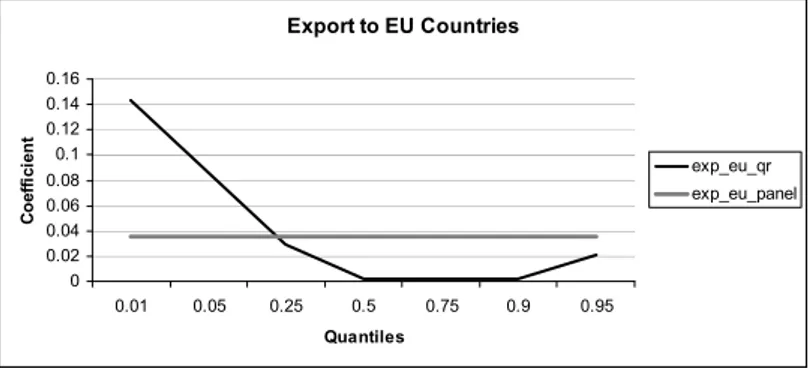
In this section, we firstly run a panel model (GLS, fixed effects) on manufac-turing where the dependent variable (log of labor productivity) is regressed on a set of covariates, including a non linear term for human capital. Secondly, we highlight the bias in GLS estimates by running the same model using quantile re-gressions for panel data. We present results from manufacturing, exporters and non exporters and a focus on food, textiles and mechanics. For ease of compre-hension, tables with models estimates are reported in Appendix A, while in this section we discuss the graphical representation comparing GLS and quantile re-gressions estimates. These graphs report the quantiles of the distribution on the horizontal axis and the estimates value, on the vertical axis. GLS estimates are presented as horizontal lines and their constant values show that they are not able to capture the whole story. The quantile regression curves show, instead, that the value of the estimated coefficients vary over the conditional labor productivity distribution. The closer the two lines, the better the GLS estimates capture the conditional labor productivity dynamics.

(14)

5.2.1 Results: Manufacturing

In Table A.1, we report the results from panel regressions with fixed effects (time) both in linear and non linear specifications (for the human capital compo-nent) for manufacturing sectors2_{. Results show that physical and human capital}

are particularly relevant in manufacturing. The human capital component in manufacturing has a non linear effect, showing a peak (maximum): on average the labor productivity grows until a ratio of white collars equal to 75% of blue collars. Investments in R&D internationalization and patents are extremely important in manufacturing. Focusing on exporting firms (specification (3)), we notice that while the effect of physical capital invested is lower than for manufacturing firms as a whole, the role of human capital and investment in R&D as well as innova-tiveness increases.

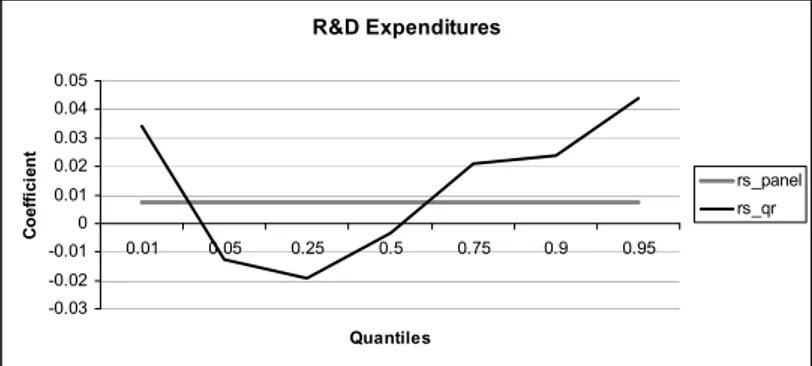
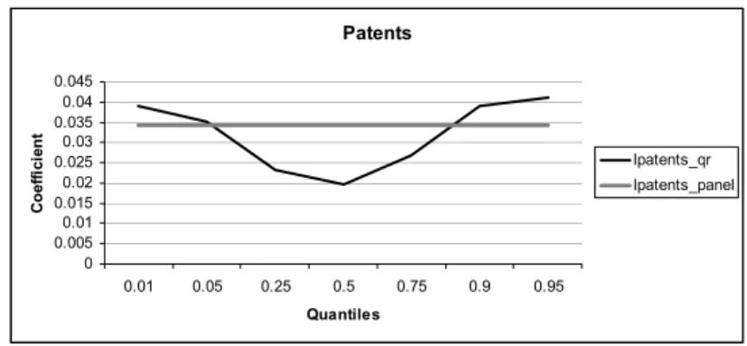
This first round of results point out some general characteristics of Italian firms and suggesting a policy to stimulate the Italian labor productivity. However, whilst standard regression analyses focus on the labor productivity of the mean firm, such techniques may be inappropriate given that its distribution is not nor-mally distributed. Quantile regressions, instead, allow us to parsimoniously de-scribe the importance of a set of variables over the entire conditional labor pro-ductivity distribution, and the graphical representation shows that the average ef-fect estimated of covariates via GLS does not fully capture the labor productivity conditional distribution dynamics. For example, as reported in Figure 6, the inno-vativeness proxy (number of patents registered) effect is very close to the GLS estimate when the quantile regression solution is evaluated at the median firm (i.e. at the 50% quantile), while it becomes much more important at 90% quantile and much less relevant for low productivity firms (1% or 5% quantiles). The human capital proxy in Figure 4 has a similar behavior, as for low productivity firms it has a little impact on labor productivity but this effect rises as quantiles rise. Note that, from the quantile regressions estimates, the role of internationalization on labor productivity (Figures 7 and 8) is much more important for low productive firms than for highly productive firms. This means that, low productive firms should invest on their role in international markets and on investments to in-crease their productivity and that the expected effects are larger than for highly productive firms. These results show how standard approaches do not fully ex-plain the labor productivity dynamics of Italian firms and how the performance of low and high labor productivity firms strongly differ. In particular, low pro-ductivity firms would highly benefit, in terms of increasing propro-ductivity, from in-vestments in physical capital and internationalization, while high productivity firms would benefit more from investments in R&D and innovativeness as well as investments in human capital.

2_{Panel and quantiles regressions have been run also on service sectors with the same} specifica-tion we used to describe manufacturing behavior. We preferred not to include these results in this version of the paper because a deep and exhaustive analysis on service sectors would have re-quested additional and different specifications. For space reasons, we leave this for future research. However, models results on service sectors are available from authors upon request.

(15)

5.2.2 Results: Exporters and Non Exporters

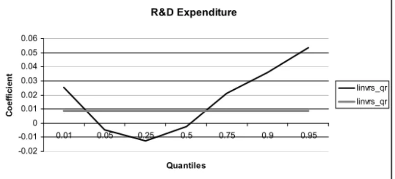
Focusing on the quantile regressions results from exporters and non exporters (Tables A.3 and A.4), we show that human capital is particularly relevant for non exporters that compete only within the national boundaries while innovativeness becomes crucial for exporters. Figures from 8 to 11 report the comparison be-tween GLS and quantile regressions estimates for exporters showing that invest-ments in both physical and human capital and R&D expenditures have a higher impact for highly productive exporters while the role of innovativeness (number of patents registered) has a strong impact on both low and high productive firms while it has a lower effect on median firms. This is very interesting because it shows that if we only focus on GLS estimates we would attribute to innovative-ness a weaker role than it really has on specific groups of firms.

5.2.3 Results: A Focus on Sectors

In this section, we focus on three of the most important sectors for the Italian export (in terms of propensity to export): food, textiles and mechanical machin-ery.

These sectors are leaders in international markets and represent a worldwide famous brand of the so called “Made in Italy”. From our results, reported in Ta-bles from A.5 to A.7, we notice that innovativeness, human capital and interna-tionalization have a role on fostering labor productivity of these sectors but with strong heterogeneity across industries and quantiles. In particular, all sectors have a maximum on the human capital proxy, showing that the higher the number of white collars compared to blue collars the higher the average labor productivity, possibly thanks to an increased level of efficiency of labor and procedures. This effect is non linear and it is very different from one sector to another3_{. In other}

words, there exist a level above which the cost of hiring new skilled workers turns out to be higher than the benefits the firms receive in terms of higher sales per worker (Giovannetti et al., 2011). Patents registered and internationalization are key variables in stimulating the labor productivity of firms in these sectors but with different impact. For instance, innovativeness in food sector is significant for low and high productivity firms but it turns out to be irrelevant for the me-dian firm, confirming the need of a quantile regression approach; in textiles, in-stead, the effect of innovation grows as productivity grows. More productive tex-tiles firms strongly benefit from innovations. On the contrary, in the machinery sector, patents are significant only for median firms and have very little impact on both low and high productivity firms. Internationalization, instead, is crucial es-pecially for low productivity firms in all sectors but export outside Europe is par-ticularly important for food firms that have on average larger markets than other sectors.

3_{Further analysis on non-linearities in these models, results and discussion are available from} au-thors upon request.

(16)

Investments 0 0.01 0.02 0.03 0.04 0.05 0.01 0.05 0.25 0.5 0.75 0.9 0.95 Quantiles C o ef fi ci en t lk_qr lk_panel

Figure 3 – Quantile Regressions versus Panel Regression estimates: Physical Capital.

Ratio White to Blue Collars

0 0.02 0.04 0.06 0.08 0.1 0.12 0.01 0.05 0.25 0.5 0.75 0.9 0.95 Quantiles C o ef fi ci en t ratio_wtob_qr ratio_wtob_panel

Figure 4 – Quantile Regressions versus Panel Regression estimates: Human Capital.

R&D Expenditures -0.03 -0.02 -0.01 0 0.01 0.02 0.03 0.04 0.05 0.01 0.05 0.25 0.5 0.75 0.9 0.95 Quantiles C o ef fi ci en t rs_panel rs_qr

(17)

Patents 0 0.005 0.01 0.015 0.02 0.025 0.03 0.035 0.04 0.045 0.01 0.05 0.25 0.5 0.75 0.9 0.95 Quantiles C o effi ci en t patents_qr patents_panel

Figure 6 – Quantile Regressions versus Panel Regression estimates: Patents Registered.

Export to Extra EU Countries

0 0.02 0.04 0.06 0.08 0.1 0.12 0.14 0.01 0.05 0.25 0.5 0.75 0.9 0.95 Quantiles C o ef fi ci en t exp_extraeu_qr exp_extraeu_panel

Figure 7 – Quantile Regressions versus Panel Regression estimates: Export to Countries outside the EU. Export to EU Countries 0 0.02 0.04 0.06 0.08 0.1 0.12 0.14 0.16 0.01 0.05 0.25 0.5 0.75 0.9 0.95 Quantiles C o eff ici en t exp_eu_qr exp_eu_panel

(18)

Investments -0.04 -0.02 0 0.02 0.04 0.06 0.08 0.1 0.01 0.05 0.25 0.5 0.75 0.9 0.95 Quantiles C o ef fi ci en t lk_qr lk_panel

Figure 9 – Quantile Regressions versus Panel Regression estimates for Exporters: Physical Invest-ments.

Ratio White to Blue Collars

0 0.02 0.04 0.06 0.08 0.1 0.12 0.01 0.05 0.25 0.5 0.75 0.9 0.95 Quantiles C o ef fi ci en t ratio_wtob_qr ratio_wtob_panel

Figure 10 – Quantile Regressions versus Panel Regression estimates for Exporters: Human Capital.

R&D Expenditure -0.02 -0.01 0 0.01 0.02 0.03 0.04 0.05 0.06 0.01 0.05 0.25 0.5 0.75 0.9 0.95 Quantiles C o ef fi ci en t linvrs_qr linvrs_qr

Figure 11 – Quantile Regressions versus Panel Regression estimates for Exporters: R&D Expendi-tures.

(19)

Patents 0 0.005 0.01 0.015 0.02 0.025 0.03 0.035 0.04 0.045 0.01 0.05 0.25 0.5 0.75 0.9 0.95 Quantiles C o ef fi ci en t lpatents_qr lpatents_panel

Figure 12 – Quantile Regressions versus Panel Regression estimates for Exporters: Patents.

6. CONCLUSIONS

During the last decades the Italian economy experienced a strong decline in its economic growth rates. The literature usually attributes this to the characteristics of the Italian productive system based on low labor productivity rate and high specialization in traditional, low-tech sectors.

This paper deals with the heterogeneous performance of Italian firms’ labor productivity and investigates how firms characteristics affect the dynamics of the Italian firms’ labor productivity in recent years (1998-2004). We use an original panel recently developed by the Italian National Institute of Statistics at a micro level (firm level) including information from their balance sheets and internation-alization activity. In particular, we use a non linear Cobb-Douglas production function and a quantile regression approach to test how a set of firms’ character-istics influences the Italian firms labor productivity growth in the period consid-ered. We run models on manufacturing and focus on three of the most interna-tionalized sectors in Italy (food, textiles and mechanical machinery).

We find that labor productivity is very heterogeneous and that the relation-ships between labor productivity and firms characteristics are not constant across quantiles. We disentangle the effect of a set of variables on different levels of la-bor productivity; we show that what is relevant for highly productive firms may not work for low productive firms. Using the quantile regression approach we show that the medium estimates obtained with GLS do not capture the complex dynamics and heterogeneity of the Italian firms labor productivity. Innovative-ness and human capital, in particular, have a larger impact on fostering labor pro-ductivity of low productive firms than that of high productive firms. A similar re-sult is detected for exporter and non exporters: human capital and innovation have a higher impact for exporters than for non exporters. The role of interna-tionalization on labor productivity is more important for low productive firms than for highly productive firms, suggesting that low productive firms should ex-pand their role in international markets to increase their productivity and that the expected effects are larger than for highly productive firms.

(20)

The focus on specific sectors shows that innovativeness, human capital and in-ternationalization have a role on fostering labor productivity, with large discrep-ancy both across industries and quantiles. Innovativeness in food sector is polar-ized: it is significant for low and high productivity firms but it turns out to be ir-relevant for the median firm. In textiles, instead, the effect of innovation grows as productivity grows. In the machinery sector, instead, patents are significant only for median firms and have very little impact on both low and high productivity firms. Internationalization, instead, is crucial especially for low productivity firms in all sectors.

Department of Economics, New York University MARGHERITA VELUCCHI

and Dipartimento di Statistica “G. Parenti” Università di Firenze

velucchi@ds.unifi.it

Dipartimento di Statistica “G. Parenti” ALESSANDRO VIVIANI

Università di Firenze viviani@ds.unifi.it

REFERENCES

ARNOLD J.M., HUSSINGER K., (2005), Export Behavior and Firm Productivity in German Manufacturing: A Firm-level Analysis, Review of World Economics, 141 (2), pp. 219-243. BARRO R. J., (1999), Notes on Growth Accounting, Journal of Economic Growth, 4(2), pp.

119-137.

BIFFIGNANDI S. ZELI A., (2010), Integrating databases over time: what about representativity in panel data?, presented at Third International Workshop on Business Data Collection Meth-odology April 28-30, 2010, Destatis, Wiesbaden, Germany.

BUCHINSKY M., (1994), Changes in the U.S. wage structure 1963-1987: application of quan-tile regression, Econometrica, 62, pp. 405-458.

BUCHINSKY M., (1998), Recent advances in quantile regression models: a practical guide for empirical research, Journal of Human Resources, 33 (1), pp. 88-126.

CASTELLANI D., GIOVANNETTI G., (2010), Productivity and the international firm: dissecting heterogeneity, Journal of Economic Policy Reform, 13(1), pp. 25-42.

CAVES, D., CHRISTENSEN L., DIEWERT E. (1982a), The Economic Theory of Index Numbers and the Measurement of Input, Output and Productivity, Econometrica 50 6, pp. 1393-1414.

CAVES, D., CHRISTENSEN L., DIEWERT E., (1982b), Multilateral Comparisons of Output, Input and Productivity Using Superlative Index Numbers, The Economic Journal, 92, pp. 73-86. COELLI T., PRASADA RAO D.S., BATTESE G.S. (1998), An Introduction to Efficiency and Productivity

Analysis, Kluwer Academic Publishers.

DOSI G., GRAZZI M., TOMASI C., ZELI A., (2010), Turbulence underneath the big calm? Explor-ing the micro-evidence behind the flat trend of manufacturExplor-ing productivity in Italy, LEM Working Paper Series, 2010/03.

EICHER T., STROBEL T., (2008), The Rise and Fall of German Productivity: Software Invest-ment as the Decisive Driver, CESifo Economic Studies, 54(3), pp. 386-413.

FERRANTE M.R., FREO M. (2010), Measuring the “net” productivity premium of international-ized firms: a quantile regression decomposition approach, paper presented at ETSG

(21)

2010 Lausanne Twelfh Annual Conference 9-11 September 2010, University of Lausanne.

FRYGES H., WAGNER J.,(2008), Exports and Productivity Growth: First Evidence from a Continuous Treatment Approach, Review of World Economics, 144 (4), pp. 695-722. GALOR, O.(2005), The Transition from Stagnation to Growth: Unified Growth Theory, in

P. Aghion and S.N. Durlauf, eds., Handbook of Economic Growth, Volume 1A, Amster-dam, North Holland, pp. 171-293.

GRASSINI L., MARLIANI G., (2009), Italian Labour Productivity Changes: An Analysis of Firm Survey Data 1998-2004, in A. Viviani (eds.), Firms and system competitiveness in Italy, Firenze University Press, Firenze, pp. 39-56.

GRIFFITH R., REDDING S., VAN REENEN J. (2004), Mapping the Two Faces of R&D: Productiv-ity Growth in a Panel of OECD Industries, Review of Economics and Statistics, 86(4), pp. 883-895.

HALL B.H., LOTTI F., STROBELY T., (2009) Innovation and productivity in SMEs: empirical evi-dence for Italy, Small Business Economics, 33, 1, pp. 13-33.

HANSEN T., (2010), Exports and Productivity: An Empirical Analysis of German and Aus-trian Firm-level Performance.

HAO L., NAIMAN D. Q.,(2007), Quantile Regression, Sage Publications, Thousand Oaks.

HULTEN C. (2001), Total Factor Productivity. A Short Biography, in New Developments in Productivity Analysis, Hulten C., Dean E.R. Harper M.J. (eds.) National Bureau of Eco-nomic Research, University of Chicago Press, pp. 1-54.

ITALIAN INSTITUTE FOR FOREIGN TRADE, (2010), L’Italia nell’economia internazionale, Rapporto ICE 2009-2010, Roma.

KLEINKNECHT A., MOHNEN P. (2002), (eds.), Innovation and Firm Performance, London, Palgrave. KOENKER R., BASSETT G., (1978), Regression quantiles, Econometrica, 46, pp. 33-50.

KOENKER R., HALLOCK K. F., (2001), Quantile Regression, Journal of Economic Perspectives, 15, 4, pp. 143-156.

KOENKER R.,(2005), Quantile Regression Cambridge University Press, New York.

MAYER T., OTTAVIANO g.m. (2008), The Happy Few the internationalization of European Firms, Bruegel blueprint series, n. 3.

MELITZ M.,(2003), The impact of trade on intra-industry reallocations and aggregate indus-try productivity, Econometrica, 71, pp. 1695-725.

NARDECCHIA R, SANZO R., ZELI A., (2010), La costruzione di un panel retrospettivo di micro-dati per le imprese italiane con 20 addetti e oltre dal 1998 al 2004, Rapporto di ricerca, ISTAT, Roma.

OECD, (2001), Measuring Productivity: OECD Manual-Measurement of Aggregate and Industry-Level Productivity Growth. Paris.

PROIETTI T., MUSSO A., (2007), Growth Accounting For the Euro Area: A Structural Ap-proach, ECB Working Papers Series,804 August 2007.

SUMMARY

Determinants of the Italian labor productivity: a quantile regression approach

This paper investigates how some firms’ characteristics affect the dynamics of the Ital-ian firms’ labor productivity in recent years (1998-2004) using an original panel from the Italian National Institute of Statistics at a micro level (firm level). The original database and a quantile regression approach allow us to highlight that labor productivity is very heterogeneous and that the relationship between labor productivity and firms

(22)

characteris-tics is not constant across quantiles. We show that estimates obtained via GLS do not capture the complex dynamics and heterogeneity of the Italian firms labor productivity. Innovativeness and human capital, in particular, have a larger impact on fostering labor productivity of low productive firms than that of high productive firms. Finally, we focus on three highly internationalized sectors and show that innovativeness, human capital and internationalization have a role on fostering labor productivity, with large discrepancy both across industries and quantiles.

(23)

APPENDIX A TABLE A.1

Model Results for different specifications: Manufacturing (1), Manufacturing non linear (2), Exporting Firms (3)

(1) (2) (3)

Variables Llabprod llabprod llabprod

Lk(-1) 0.023*** 0.027*** 0.028*** (0.0132) (0.022) (0.024) Ratio_wtob 0.00836*** 0.0200*** 0.0200*** (0.00301) (0.00551) (0.00551) ratio_wtob2 -0.000133** -0.000133** (5.31e-05) (5.31e-05) Linvrs(-1) 0.0067* 0.0076* 0.0089* (0.0018) (0.0022) (0.0018) Lpatents(-1) 0.0257*** 0.0293*** 0.0343*** (0.00615) (0.00615) (0.00615) lprim_extraeu 0.0124** 0.0125** 0.0125** (0.00515) (0.00516) (0.00516) lprim_eu 0.0478*** 0.0482*** 0.0482*** (0.00705) (0.00706) (0.00706) lprex_extraeu 0.0264*** 0.0267*** 0.0267*** (0.00731) (0.00732) (0.00732) lprex_eu 0.0357*** 0.0359*** 0.0359*** (0.00753) (0.00753) (0.00753) Constant 3.696*** 3.695*** 3.695*** (0.0998) (0.0995) (0.0995)

Fixed Effect YES YES YES

Observations 1,863 1,863 1,863

Number of codice 1,137 1,137 1,137

Standard errors in parentheses *** p<0.01, ** p<0.05, * p<0.1

TABLE A.2

Quantile Regression Results for Manufacturing

(1) (2) (3) (4) (5) (6) (7)

Variables llabprod llabprod llabprod llabprod llabprod Llabprod llabprod Quantiles 0.01 0.05 0.25 0.5 0.75 0.9 0.95 Lk(-1) 0.0455** 0.0237** 0.00991 0.0365 0.0333 0.00842 0.00938** (0.091) (0.085) (0.095) (0.156) (0.202) (0.280) (0.530) ratio_wtob 0.0407 0.0202 0.0745*** 0.0759*** 0.0728*** 0.110*** 0.106*** (0.0438) (0.0238) (0.00874) (0.00920) (0.00816) (0.0103) (0.0121) Ratio_wtob2 -0.0002 -0.0008 -0.0009*** -0.0009*** -0.0006*** -0.001*** -0.001*** (0.00043) (0.000236) (8.48e-05) (0.000103) (7.72e-05) (0.000101) (0.000118) Linvrs(-1) 0.0342 -0.0125 -0.0194*** -0.0035 0.021 0.0239* 0.0437 (0.0547) (0.0182) (0.00633) (0.00749) (0.00892) (0.0122) (0.0211) Lpatents(-1) 0.0389 0.0352 0.0233*** 0.0198*** 0.0268*** 0.0389*** 0.0412* (0.0605) (0.0636) (0.00681) (0.00798) (0.0023) (0.0117) (0.0134) lprim_extraeu 0.0129 -0.0159 0.00698 0.0146* 0.00550 -0.00109 -0.00570 (0.0430) (0.0173) (0.00579) (0.00763) (0.00967) (0.0141) (0.0260) lprim_eu 0.0286 0.0537** 0.0480*** 0.0778*** 0.0992*** 0.0868*** 0.0932** (0.0520) (0.0233) (0.00797) (0.0109) (0.0150) (0.0221) (0.0386) lprex_extraeu 0.119** 0.0763*** 0.0416*** 0.0421*** 0.0305** 0.0198 0.00569 (0.0562) (0.0255) (0.00893) (0.0111) (0.0135) (0.0188) (0.0323) lprex_eu 0.143*** 0.0856*** 0.0292*** 0.00167 0.00245 0.00213 0.0213 (0.0402) (0.0271) (0.00887) (0.0114) (0.0143) (0.0216) (0.0371) Constant 1.453* 2.591*** 3.729*** 4.241*** 4.477*** 4.604*** 4.861*** (0.809) (0.279) (0.0838) (0.101) (0.122) (0.170) (0.256)

Note: Quantile regressions identify the coefficients for firms at the z-th quantile of the productivity distribution. All regressions

are panel regressions, SEs in brackets. Robust SEs were applied allowing for correlation within industries over time. SEs for quantile regressions are derived via bootstrap techniques for 1000 replications. Standard errors in parentheses. Significance lev-els: *** p<0.01, ** p<0.05, * p<0.1

(24)

TABLE A.3

Quantile Regression Results for Exporting Firms

(1) (2) (3) (4) (5) (6) (7)

Variables llabprod Llabprod Llabprod llabprod llabprod llabprod Llabprod Quantiles 0.01 0.05 0.25 0.5 0.75 0.9 0.95

Lk(-1) -0.0165 -0.0156 0.0141 0.0335 0.0443 0.0542 0.0838

(0.0552) (0.0287) (0.00779) (0.0311) (0.0322) (0.0554) (0.0186) ratio_wtob 0.0155** 0.0075*** 0.0109*** 0.0123*** 0.0312*** 0.0365*** 0.0389*** (0.00737) (0.00266) (0.00297) (0.00267) (0.00231) (0.00283) (0.00339) ratio_wtob2 -3.16e-05** -1.58e-05*** -2.46e-05*** -2.38e-05*** -5.87e-05*** -6.94e-05*** -7.48e-05***

(1.39e-05) (5.11e-06) (5.65e-06) (4.91e-06) (4.30e-06) (5.27e-06) (6.33e-06)

Linvrs(-1) 0.0122 -0.0046 -0.0124 -0.0025 0.021* 0.0359* 0.0537* (0.0294) (0.0157) (0.00440) (0.00250) (0.00634) (0.0145) (0.011) Lpatents(-1) 0.0339 0.0284** 0.0368*** 0.0332*** 0.0367*** 0.0397*** 0.0494*** (0.0543) (0.0125) (0.00533) (0.00609) (0.00682) (0.0112) (0.0168) lprim_extraeu -0.0141 0.00355 0.00812* 0.0142** 0.0204*** 0.0265** 0.0249 (0.0406) (0.00993) (0.00448) (0.00556) (0.00681) (0.0122) (0.0184) lprim_eu 0.0870* 0.0521*** 0.0643*** 0.0781*** 0.0920*** 0.0867*** 0.103*** (0.0489) (0.0118) (0.00583) (0.00756) (0.0100) (0.0182) (0.0298) lprex_extraeu 0.110* 0.0428*** 0.0359*** 0.0356*** 0.0240** 0.00543 0.007** (0.0659) (0.0132) (0.00632) (0.00781) (0.00949) (0.0168) (0.0249) lprex_eu 0.103 0.0774*** 0.0207*** 0.00314 0.0136 0.00978 0.01*** (0.0695) (0.0142) (0.00683) (0.00834) (0.0102) (0.0177) (0.0271) Constant 2.042** 3.061*** 3.958*** 4.428*** 4.701*** 4.910*** 4.934*** (0.853) (0.156) (0.0635) (0.0734) (0.0871) (0.141) (0.199)

TABLE A.4

Quantile Regression Results for Non Exporting Firms

(1) (2) (3) (4) (5) (6) (7)

Variables llabprod Llabprod llabprod llabprod llabprod llabprod llabprod Quantiles 0.01 0.05 0.25 0.5 0.75 0.9 0.95

Lk(-1) 0.000382 0.0516 0.0339 0.0290 0.104** 0.0623 0.103***

(0.00342) (0.121) (0.0466) (0.0696) (0.0439) (0.0784) (0.0332) ratio_wtob -0.00927*** -0.0477** -0.00817 0.00228 0.0111 0.0588*** 0.0599***

(0.000839) (0.0200) (0.0107) (0.0158) (0.0118) (0.0106) (0.00649) ratio_wtob2 4.08e-05*** 0.000210** 1.71e-05 1.51e-05 -2.44e-05 -0.000206*** -0.000215***

(3.61e-06) (8.13e-05) (4.50e-05) (6.01e-05) (4.67e-05) (4.16e-05) (2.37e-05)

Linvrs(-1) -0.139*** -0.0672 -0.0233 0.0161 0.00446 -0.0197 -0.0340 (0.00219) (0.108) (0.0368) (0.0466) (0.0293) (0.0434) (0.0319) Lpatents(-1) 0.119*** 0.0760 0.0116 0.0728 0.0963*** 0.0196 -0.00576 (0.00263) (0.0965) (0.0419) (0.0548) (0.0356) (0.0603) (0.0323) lprim_extraeu 0.290*** 0.188*** 0.141*** 0.0850** 0.0806*** 0.0189 0.0440 (0.00207) (0.0653) (0.0267) (0.0417) (0.0298) (0.0504) (0.0406) lprim_eu -0.109*** -0.0955** -0.0228 0.00654 0.0157 0.0358 0.0261 (0.00219) (0.0479) (0.0289) (0.0446) (0.0302) (0.0594) (0.0516) Constant 3.245*** 3.491*** 4.048*** 4.331*** 3.921*** 5.214*** 5.063*** (0.0288) (0.896) (0.417) (0.591) (0.374) (0.602) (0.214)

(25)

TABLE A.5

Quantile Regression Results for selected sectors: Food

(1) (2) (3) (4) (5) (6) (7)

Variables llabprod llabprod llabprod llabprod llabprod llabprod llabprod Quantiles 0.01 0.05 0.25 0.5 0.75 0.9 0.95 Lk(-1) 0.125*** 0.211 -0.0169 0.0455 0.0671 0.142 0.187 (0.00572) (0.140) (0.130) (0.0521) (0.0504) (0.115) (0.204) ratio_wtob 0.407*** 0.0188 1.004 1.060*** 0.734** 1.960*** 2.446*** (0.0332) (0.697) (0.732) (0.300) (0.284) (0.669) (0.834) ratio_wtob2 0.0237 0.126 -0.324 -0.279** -0.0941 -0.639** -0.800** (0.0149) (0.310) (0.323) (0.132) (0.116) (0.271) (0.314) Linvrs(-1) -0.029*** -0.0011 -0.0167 -0.0212 -0.0256 -0.0269 -0.0449 (0.00258) (0.137) (0.0619) (0.0236) (0.0274) (0.0613) (0.0683) Lpatents(-1) 0.0417*** 0.0505 0.0162 0.0783 0.0621 0.0401* 0.0754*** (0.00333) (0.138) (0.0919) (0.0300) (0.0292) (0.0106) (0.0325) lprim_extraeu 0.125*** 0.0424 -0.0467 -0.06*** -0.0264 -0.0429 0.00671 (0.00231) (0.109) (0.0655) (0.0220) (0.0220) (0.0394) (0.0346) lprim_eu 0.0282*** 0.190* 0.209** 0.175*** 0.0974** 0.0915 0.0264 (0.00380) (0.103) (0.0909) (0.0351) (0.0418) (0.0756) (0.0422) lprex_extraeu 0.191*** 0.0878* 0.0162 0.00454 0.0517* 0.185*** 0.191*** (0.00324) (0.0506) (0.0609) (0.0281) (0.0275) (0.0583) (0.0545) lprex_eu 0.0373*** -0.0732 0.0512 0.0857** 0.108*** 0.0970 0.107** (0.00366) (0.116) (0.0796) (0.0336) (0.0322) (0.0652) (0.0535) Constant 0.832*** 2.083 3.293*** 3.259*** 4.213*** 4.599*** 5.029*** (0.0383) (1.710) (0.968) (0.357) (0.345) (0.763) (1.160)

TABLE A.6

Quantile Regression Results for selected sectors: Textiles

(1) (2) (3) (4) (5) (6) (7)

Variables Llabprod llabprod llabprod llabprod Llabprod llabprod llabprod Quantiles 0.01 0.05 0.25 0.5 0.75 0.9 0.95 Lk(-1) 0.0059*** 0.00288 0.0154 0.101*** 0.210*** 0.190*** 0.164 (0.00442) (0.0587) (0.0284) (0.0490) (0.0425) (0.0343) (0.164) ratio_wtob -0.150*** -0.0790 0.0619* 0.179*** 0.196*** 0.320*** 0.296*** (0.00476) (0.120) (0.0343) (0.0545) (0.0342) (0.0240) (0.0793) ratio_wtob2 0.00595*** 0.00374 -0.000135 -0.00364** -0.00435*** -0.00790*** -0.00749*** (0.000128) (0.00324) (0.00093) (0.00147) (0.000930) (0.000642) (0.00223) Linvrs(-1) -0.0236*** -0.00058 -0.000657 0.00354 0.0242 0.0286 0.0677 (0.0024) (0.027) (0.0367) (0.0452) (0.0286) (0.0352) (0.278) Lpatents(-1) 0.00567*** 0.0371 0.0770*** 0.098** 0.0994*** 0.113*** 0.117* (0.0022) (0.058) (0.012) (0.0312) (0.0234) (0.0750) (0.079) lprim_extraeu 0.0398*** -0.0382 -0.0221 0.00667 0.0248 0.0146 0.0173 (0.00255) (0.0396) (0.0167) (0.0288) (0.0293) (0.0268) (0.0826) lprim_eu 0.0104*** 0.0646 0.0359 0.0711* 0.0263 0.0241 0.0721 (0.00341) (0.0537) (0.0226) (0.0373) (0.0377) (0.0292) (0.132) lprex_extraeu 0.0623*** 0.0196 0.0135 0.0319 0.0518 0.0678** 0.0981 (0.00354) (0.0657) (0.0254) (0.0379) (0.0316) (0.0304) (0.168) lprex_eu 0.168*** 0.233*** 0.150*** 0.107*** 0.0975*** 0.107*** 0.0352 (0.00338) (0.0412) (0.0235) (0.0367) (0.0288) (0.0277) (0.119) Constant 2.066*** 1.966*** 3.215*** 4.598*** 4.502*** 4.303*** 4.690*** (0.0297) (0.646) (0.221) (0.338) (0.298) (0.264) (1.191)

(26)

TABLE A.7

Quantile Regression Results for selected sectors: Mechanics

(1) (2) (3) (4) (5) (6) (7)

Variables llabprod llabprod llabprod llabprod Llabprod llabprod Llabprod Quantiles 0.01 0.05 0.25 0.5 0.75 0.9 0.95 Lk(-1) 0.0657 0.0218 0.0201 0.033* 0.0593*** 0.067* 0.0658 (0.123) (0.0567) (0.0158) (0.0181) (0.0196) (0.0342) (0.0701) ratio_wtob 0.273*** 0.213*** 0.0980*** 0.135*** 0.126*** 0.111*** 0.0866 (0.0799) (0.0629) (0.0236) (0.0220) (0.0213) (0.0326) (0.0688) ratio_wtob2 -0.0125*** -0.0116*** -0.00221*** -0.00369*** -0.00371*** -0.00356*** -0.00290 (0.0031) (0.00237) (0.000658) (0.000796) (0.000583) (0.00217) (0.00386) Linvrs(-1) -0.00267 0.00157 -0.00798 0.00562 0.00678 0.0189 0.0256 (0.0492) (0.0268) (0.00723) (0.00787) (0.00771) (0.0119) (0.0230) Lpatents(-1) 0.0146 0.0168 0.0317*** 0.0195** 0.0255*** 0.0257* 0.0389 (0.0532) (0.0387) (0.00734) (0.00854) (0.00765) (0.0219) (0.0103) lprim_extraeu -0.0119 0.0128 0.00864 0.00960 0.0187** 0.0187 0.0379 (0.0430) (0.0293) (0.00780) (0.00867) (0.00880) (0.0142) (0.0300) lprim_eu -0.0291 0.0364 0.0317*** 0.0489*** 0.0573*** 0.0738*** 0.0619 (0.0594) (0.0313) (0.00982) (0.0113) (0.0119) (0.0223) (0.0407) lprex_extraeu 0.109 0.0214 0.0133 0.0218* 0.0168 0.0418* 0.0276 (0.0675) (0.0337) (0.0108) (0.0126) (0.0131) (0.0232) (0.0409) lprex_eu 0.280*** 0.110*** 0.0814*** 0.0651*** 0.0485*** 0.00664 0.026*** (0.0795) (0.0357) (0.0116) (0.0143) (0.0164) (0.0311) (0.0580) Constant 1.530* 3.131*** 3.872*** 4.137*** 4.646*** 4.908*** 4.983*** (0.858) (0.376) (0.0975) (0.107) (0.115) (0.194) (0.378)