Efficient coverage optimization in energy-constrained Wireless Sensor Networks

(1)

UNIVERSITY

OF TRENTO

DIPARTIMENTO DI INGEGNERIA E SCIENZA DELL’INFORMAZIONE

38100 Povo – Trento (Italy), Via Sommarive 14

http://www.disi.unitn.it

Efficient coverage optimization in energy-constrained

Wireless Sensor Networks

Luigi Palopoli, Roberto Passerone and Paolo Toldo

April 2009

Technical Report Number:

DISI-09-023

(2)

Efficient coverage optimization in energy-constrained

Wireless Sensor Networks

Luigi Palopoli

DISI - University of Trento via Sommarive 14 38100 Povo di Trento (TN),

Italy

luigi.palopoli@unitn.it

Roberto Passerone

Italy

roberto.passerone@unitn.it

Paolo Toldo

Italy

paolo.toldo@studenti.unitn.it

ABSTRACT

We consider the problem of optimizing the area coverage of a wireless sensor network under energy consumption con-straints. Following existing approaches, we use a mixed in-teger linear program formulation. We then show how to use partitioning techniques, developed in the context of VLSI place and route, to decompose the problem into separate sub-problems, overcoming the exponential complexity typ-ical of integer linear programming, while minimizing the loss in optimality. In addition, we are able to evaluate the achieved degree of optimality by computing relatively tight bounds with respect to the optimal solution. Finally, we em-ploy simple but effective heuristics to further improve our solution. The results show that our procedure is very ef-ficient and is able to find solutions that are very close to optimal.

Categories and Subject Descriptors

C.3 [Computer System Organization]: Special-purpose and application-based systems Real-time and embedded sys-tems; G.1.6 [Numerical Analysis]: Optimization integer programming

General Terms

Algorithms, Design, Performance

Keywords

Energy aware, scheduling, coverage, optimization, partition-ing, Wireless Sensor Networks

1. INTRODUCTION

Among embedded devices, wireless sensor networks (WSN) are emerging as one of the most interesting innovations in terms of potential areas of application and impact in fields such as security, health care, disaster management, agricul-tural monitoring and building automation. The most rele-vant feature of a WSN is that it is a dynamic distributed system, in which complex tasks are performed through the coordinated action of a large number of small autonomous devices (nodes). In this paper, we address the problem of maximizing the lifetime of the network which is typically bounded by the available energy in the node, especially when the system is deployed in a remote environment and/or when maintenance and battery replacement is costly. The objec-tive is therefore to design distributed algorithms for data

processing and resource management that attain an opti-mal trade-off between functionality, robustness and energy consumption.

A popular way for pursuing this result is the application of “duty-cycling”. The idea is to keep a node inactive for a long period of time when its operation is not needed, and then to awake it for a short interval to perform its duties (e.g., to sense the surrounding environment). Here we fo-cus on the problem of determining a sequence of wake-ups which maximizes the average area “sensed” by the network given a desired value for the lifetime. Several methods have been developed to solve this problem. In general, these can be classified as centralized techniques, which make use of global information about the deployment, and distributed techniques, which are typically limited by network connec-tivity, but can more easily adapt to changes in the network. In all cases the result is a static or dynamic pattern of acti-vations (schedule) for the nodes that determines their active and sleep times.

Our work falls in the category of centralized off-line tech-niques, which are most appropriate for static deployments in relatively controlled environments, such as applications in industrial automation or building management. In this case, an off-line method may provide a higher degree of optimiza-tion and avoid costly (also in terms of energy consumpoptimiza-tion) message exchanges required to perform the on-line computa-tion. This problem may be solved exactly as a mixed integer linear program (MILP), but this approach is impractical for networks with a large number of nodes due to the inherent exponential computational complexity. Instead, we are in-terested in near optimal optimization algorithms that are able to scale well with the size of the deployment.

In this paper, we start from the MILP formulation pro-posed in [9] (which will be summarized in details in Sec-tion 2) and show how to (SecSec-tion 3): (i) partiSec-tion the prob-lem into smaller sub-probprob-lems which are more easily handled by optimization algorithms, thus drastically reducing com-plexity, (ii) compute bounds on the degree of sub-optimality that we achieve, and (iii) further optimize the result us-ing simple but effective heuristics. The main partitionus-ing task is carried out by adapting standard VLSI partitioning techniques for place and route. The results, presented in Section 4, demonstrate that our procedure is particularly efficient and the computed bounds show that we are able to find close to optimal solution. Finally, Section 5 discusses possible extensions and future work.

(3)

1.1 Related work

Slijepcevic et al. are among the first to address the prob-lem of maintaining full coverage while minimizing power consumption through an active/sleep schedule [10]. In the proposed approach, the nodes are partitioned into disjoint sets, where each set of nodes completely covers the moni-tored area. The sets are activated one at a time in a re-peating sequence, thus inducing a schedule. The authors propose a quadratic time heuristic which starts by dividing the monitored area in fields covered by exactly the same nodes. The fields covered by the least number of nodes are said to be critical. The heuristic covers the most critical fields first, recomputes the criticalities, and then proceeds by selecting a new set of nodes. The algorithm terminates when all nodes have been included in the schedule. The technique is shown to significantly improve over a simulated annealing approach, both in terms of lifetime and runtime of the optimization. However, no exact solution is derived in the paper.

The work proposed by Cardei et al. is the most related to ours in terms of optimization approach [3]. The objective of the work is to maximize the network lifetime by scheduling the activity of the nodes while maintaining full coverage of a finite set of points. This is achieved by dividing the sensors into sets which are activated sequentially. Unlike the previ-ous work, a sensor may be part of different sets (so that a node may be activated several times over a period), and the active duration for each set is computed optimally by the algorithm to maximize the lifetime. The optimization prob-lem is formulated as a MILP. To cope with the complexity of the problem, the authors develop two heuristics: the first is based on a linear relaxation, while the second is similar to that proposed by Slijepcevic and Potkonjak, where each node is only partially assigned to a set for a duration equal to a lifetime granularity parameter. While the authors do provide an exact formulation, they only present results for the two heuristics.

A different solution strategy to a very similar problem is the one advocated by Alfieri et al. [2]. The authors formulate the problem as a mixed ILP and propose a solution strategy that uses two coordinated optimization problems. With the first one, they generate tentative “subnets”, i.e., subsets of nodes that have to be switched on at the same time. The second is a linear program that computes the total time every subnet has to be active. The authors also propose a greedy heuristic, amenable to a distributed implementation, but its result can be as low as 40% of the optimal.

The same problem (i.e., maximizing the lifetime and main-taining a full coverage of a specified set of points) is ad-dressed by Liu et al. [7]. The authors propose a two step procedure. In the first step, they find an upper bound of the maximal lifetime by solving a linear program which consid-ers different types of costs (including the cost of sensing and of communication). As a result, they find a specification on the total time a node should be active, which is used in the second step to generate a schedule and a route of the messages to the base station.

Several factors distinguish our proposed technique from the existing work. First, we do not aim at maintaining full coverage of an area or of a set of points, but rather at es-tablishing a periodic schedule that guarantees the largest average coverage of an area over a scheduling period given a specified lifetime of the system. By doing so, we are able

to compute the optimal trade-off between average coverage and lifetime.

As for many approaches, and following [9]), we too formu-late the problem as a MILP, which is known to have expo-nential complexity. Our objective is to make this technique scalable to a large and dense number of nodes. To do so, in-stead of considering a continuous relaxation as in [3], we par-tition and solve separate problems in a way that minimizes the potential loss in optimality. The amount of partitioning can also be controlled to strike the desired trade-off between optimality and computational complexity. This way we can handle more complex problems than in [9], where nodes are restricted to wake up exactly once per period to decrease complexity. In addition, because we have full information on the partitioning process, we are able to compute rela-tively tight bounds with respect to the optimal solution, even when this is not known.

2. PROBLEM STATEMENT

We briefly summarize the technique proposed in [9]. We assume that a set of sensor nodes N is used to monitor a set of points P. The two sets are related by a binary coverage relation R ⊆ N × P, where (n, p) ∈ R if and only if n sees (or covers) p. We denote by r(p) the set of nodes that cover p. Points can be given a different weight (certain points may be more important than others) by a function w : P → R. For instance, if a point p represents an entire region (covered by the same nodes) then w(p) could be set to the area of that region [9]. The identification of points or regions, and the determination of their weight, is orthogonal to the technique that we present in this paper, and can be done using one of the many methods described in the literature [10, 11, 6, 9]. The system operates according to a periodic schedule. The period, called the epoch, is denoted by E. In our prob-lem, the lifetime of the system is determined by the awake or activation interval I of a node, i.e., the interval during which a node is awake in the epoch. At any time t, the set of nodes that are awake at that time defines a a cov-ering function S(t), equal to the sum of the weights of all the points covered by the nodes that are awake (clearly, the same point is not counted multiple times). The objective of the optimization is to maximize the sum over the epoch of the covered area, i.e., the integral S =RE

0 S(t). Below,

we will refer to this cost function by simply using the word “coverage”. For future purposes, it is also useful to introduce the restriction SPs(t) that considers only a subset Ps ⊆ P

in the computation of the covering function. The integral of this function over the epoch will be denoted as SPs.

We assume that the epoch is discretized into an integer number of elementary time units (slots) and that nodes wake up and go to sleep only at slot boundaries. Without loss of generality, we will consider slots of size 1. Under this assumption, we can set up our problem as a Mixed Integer Linear Program (MILP).

To this end, we introduce a set of binary coverage variables Cp,kthat are equal to 1 if point p is covered in slot k. Using

the coverage variables and the w function, the function S to be optimized can be computed as;

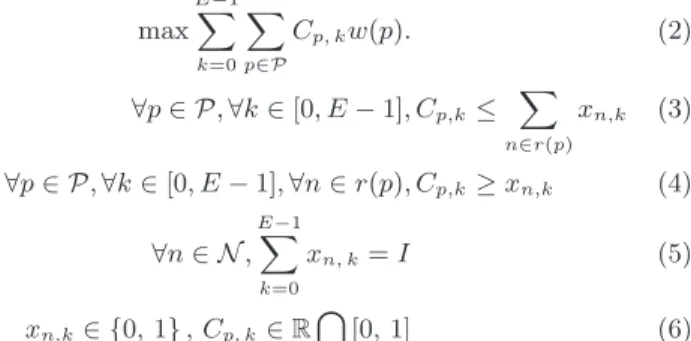
S = E−1 X k=0 X p∈P Cp, k· w(p). (1)

(4)

sched-ule. To model the schedule, we introduce a set of binary scheduling variables xn,k that are equal to 1 if node n is

active in slot k. The optimization problem can therefore be stated as follows [9]: max E−1 X k=0 X p∈P Cp, kw(p). (2) ∀p ∈ P, ∀k ∈ [0, E − 1], Cp,k≤ X n∈r(p) xn,k (3) ∀p ∈ P, ∀k ∈ [0, E − 1], ∀n ∈ r(p), Cp,k≥ xn,k (4) ∀n ∈ N , E−1 X k=0 xn, k= I (5) xn,k∈ {0, 1} , Cp, k∈ R \ [0, 1] (6) In this formulation, constraint (3), (6) are instrumental to the computation of the Cp, k variable, while constraint (5)

enforces that each node stays awake for an interval I for each epoch. Although the Cp, k variable can be relaxed to

be a continuous variable (without changing the problem), this formulation displays severe scalability issues that moti-vated our heuristic approach presented below. In the sequel, we will denote by P(N , P, ) the coverage problem defined over the sets N of nodes and P of points. Likewise, we denote by P⋆_{(N , P) the schedule of the nodes}

correspond-ing to the optimal solution. For the optimal schedule, we will denote by cP⋆_{(N , P) the value of the integral S and by}

cP⋆(N , P)|Ps(with Ps⊆ P) the value of the integral SPs.

3. A SCALABLE ALGORITHM

To efficiently solve the problem described in the previous section, we use an algorithm organized in three phases, as shown in Figure 1. The first phase consists of

partition-Figure 1: Overall optimization phases ing the set N of nodes into disjoint subsets N1, N2, . . . , Nm,

such that N =Sm

i=1Ni. We then solve the coverage

prob-lem on each partition independently, in the second phase.

Due to the exponential complexity of the MILP, the cumu-lative time required to optimize the coverage on the parti-tions is radically smaller than the one required to solve the problem as a whole. However, in order to deal with each sub-problem independently, we must neglect the interaction between nodes contained in different partition. While we partition the nodes in a way that minimizes this interaction, the solution obtained by combining the optimal schedules of the partitions is necessarily sub-optimal for the problem as a whole. In the final phase, we recombine the individual sched-ules. Remarkably, we are able to estimate upper bounds for the deviation between the optimal and the sup-optimal so-lutions. Finally, we can improve the coverage using a simple gradient descent heuristic, reducing the gap from the maxi-mum.

Clearly, the application of the divide and conquer ap-proach outlined above greatly improves the scalability of the solution, as long as the overhead incurred in the first and in the last phases can be kept in check. With this requirement in mind, we now describe each of the phases in details.

3.1 Partitioning the problem

The construction of the partition {N1, N2, . . . , Nm} out

of set N can itself be seen as a MILP optimization prob-lem. Indeed, the choice of which nodes should be placed in each partition is driven by the requirement that interactions between the nodes in the different partitions should be min-imized. This way, we can reduce the mismatch between the solution of the entire coverage problem and the aggregate so-lution of the different sub-problems (assumed independent). Roughly speaking, if two nodes cover disjoint sets of points, then their schedules can be decided independently, since the relative timing of their activations does not affect the total coverage. Conversely, if they share points in their sensing range, then they must be scheduled at different times in or-der to maximize coverage, since points that are covered by several points at the same time are counted only once. In this case we say that the two nodes interact. The strength of the interaction depends on the weight of the shared points. Since non-interacting nodes can be treated independently, they can be assigned to different partitions. The larger the interaction, instead, the more convenient it is to keep nodes in the same partition, to better account for the shared cov-erage. Thus, the goal of this phase is to find a partition that minimizes the total interaction between nodes that belong to different sets.

The optimal partitioning problem is well known in the literature, as it applies to communication design and to VLSI placement algorithms [4]. It is easy to express it as an integer linear program. Without loss of generality, consider the case of splitting the set N into two partitions N1and N2of equal

size. Let pn be a binary variable, with n ∈ N , that takes

value 0 if node n belongs to partition N1and 1 if it belongs to

partition N2. Equal size partitions can be obtained through

the following constraint: X

n∈N

pn=

|N | 2

Likewise, for each point p, we introduce two binary variables Vp(1) Vp(2)that say if point p is covered by at least one node

in one of the two partitions. Namely, Vp(1)(Vp(2)) is 1 if p is

(5)

and 0 otherwise. The two variables can be computed as: Vp(2)= _ n∈N |(n, p)∈R pn (7) Vp(1)= _ n∈N |(n, p)∈R pn, (8)

whereW denotes the OR operation and pndenotes the

logi-cal negation of pn. These two expressions can be translated

into linear constraints on the variables by standard tech-niques. In this setting, the total weight of the points seen by nodes present in both partitions is given by:P

p∈Pw(p)(V (1)

p +

Vp(2)− 1). Therefore, we obtain a Boolean Linear Program.

Although much more practical than the coverage problem (the number of variables is much smaller), the asymptotic behavior is still exponential. Luckily, there exist efficient and effective heuristics for the partitioning problem, such as the algorithm proposed by Fiduccia and Mattheyses [5], initially developed for VLSI design, which has linear com-plexity in the number of points covered by the nodes. As clearly shown in the experimental section, the price to pay in terms of distance from the optimal solution is fairly ac-ceptable.

When the number of nodes is large, partitioning can be applied recursively or the number of partitions can be in-creased to obtain separate sets of nodes with the desired size (and which can be handled by the ILP solver). This way, a trade-off can be established between optimality (with fewer partitions) and computational efficiency. We discuss how to properly combine the schedules for the different partitions later in Section 3.3.

3.2 Solving and bounding the problem

From the two partitions N1 and N2we can identify three

sets of points: P1 contains the points seen only by nodes in

N1, P2 contains the points seen only by nodes in N2, and

P1, 2 contains the points seen by nodes in both partitions.

In fact, partitioning is done so that the total weight of the nodes contained in P1,2 is minimal.

A possible solution for the coverage problem can therefore be found by solving the two problems P(N1, P1), P(N2, P2)

and then combining the two corresponding optimal sched-ules P⋆_(N

1, P1) and P⋆(N2, P2). Let P+(N , P) be the

combined schedule obtained when nodes N1 are scheduled

according to P⋆_(N

1, P1), and nodes N2 are scheduled

ac-cording to P⋆_(N

2, P2), and let cP+(N , P) be the coverage

obtained with this schedule. This solution, produced by our procedure, is necessarily suboptimal, since the schedule P+(N , P) is a feasible solution for P(N , P). More intu-itively, while the solutions of the two subproblems maximize the coverage in P1 and P2 respectively, it fails to consider

the interaction on the “overlapped” points in P1,2.

The structure of the problem, however, allows us to com-pute an upper bound on the distance between the opti-mal and the suboptiopti-mal coverage (cP⋆_{(N , P)−cP}+_{(N , P)).}

Given the optimal schedule P⋆_{(N , P), we can restrict the}

computation of the coverage to the two set P1 and P2

get-ting cP⋆_{(N , P)|}

P₁, cP⋆(N , P)|P₂respectively. Because the

sub-problems are less constrained, it follows that: cP⋆(N1, P1) ≥ cP⋆(N , P)|P₁,

cP⋆_(N

2, P2) ≥ cP⋆(N , P)|P₂. (9)

The total coverage of cP⋆_{(N , P) can be found summing up}

the three contributions of sets P1, P2 and P1,2:

cP⋆_(N_,P) ₌ cP⋆_(N ,P)|P₁+ cP ⋆_(N ,P)|P₁ (10) + cP⋆_(N ,P)|P_1,2.

Hence, in view of (9), we can write:

An upper bound for cP⋆_{(N , P)|}

P_1,2can be found assuming

that each point in P1,2is covered in a disjoint awake interval

by all the nodes that have it in their range: cP⋆(N , P)|P_1,2≤ X p∈P_1,2 min E I, |r(p)| ﬀ w(p). The cP+_{(N , P)|}

P_1,2 term can be computed directly from

the schedule P+_{(N , P). The bound B can therefore be}

computed as follows: B = X p∈P_1,2 min E I, |r(p)| ﬀ w(p) − cP+(N , P)|P_1,2

In practice, the bound assumes that the optimal solution will do as well as the sub-problems on the individual partitions (which is optimistic), and will do the absolute best on the overlaps (which is also optimistic). Our experiments show that, because the overlaps are minimized, the bounds are in practice very tight (see Section 4).

3.3 Final optimization

The obvious way to combine schedules computed inde-pendently for each partition is simply to synchronize them at the beginning of the epoch. In other words, we run the separate schedule “in phase”. This choice is, however, arbi-trary. Recall, in fact, that a schedule is periodic and that we evaluate the coverage over the entire epoch. Coverage is therefore invariant to translations of the schedule on the time axis. Indeed, the solution returned by the ILP solver is only one of several equivalent solutions that can be ob-tained by shifting the awake interval of all nodes repeatedly one slot to the right or to the left.

Coverage on points that are shared between nodes of dif-ferent partitions, however, is not optimal, and is therefore affected by changing the relative phase of the schedules. Our first heuristic to improve the solution is therefore to recom-pute the total coverage under all possible shifts, and run the schedules, possibly out of phase, for the best result. In practice, we need only recompute the coverage of the points shared by the partitions (the “overlaps”), since, as pointed out, the coverage on the partitions themselves is constant. Thus, the complexity of this computation is linear in the number of overlapping points times the number of slots in the epoch. This heuristic is particularly simple and fast, but provides excellent results. In addition, since the coverage on the individual partitions is not affected by the operation, we

(6)

can recompute tighter bounds on the solution that take the new schedule on the overlaps into account.

The extension to several schedules, obtained from a recur-sive application of the partitioning procedure, is not totally straightforward, as the number of possible relative shifts grows exponentially with the number of partitions. We have found that, empirically, it is convenient to re-phase the schedules towards the root of the partitioning tree, rather than at the bottom, to take advantage of more topology information.

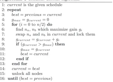
For an additional improvement, we consider the increase or decrease in coverage which results from swapping the awake time of any pair of nodes in the combined schedule. This procedure can be repeated in a gradient descent fash-ion until no more swaps provide any improvement. Inspired by the partitioning algorithms [4], we have implemented a procedure that improves on this simple heuristic, and per-forms swaps that temporarily decrease the coverage (if no other swap would increase it), in the hope that a new con-figuration is reached which will bring the gradient descent to an even better solution. This procedure, which has poly-nomial computational complexity, is shown in Algorithm 1. The procedure performs n/2 swaps per iteration, where n Algorithm 1Gradient descent algorithm

1: current is the given schedule 2: repeat

3: best = previous = current

4: gmax= gcurrent= 0

5: for(i = 0 to n/2) do

6: find na, nb which maximize gain gi

7: swap na and nbin current and lock them

8: gcurrent= gcurrent+ gi

9: if (gcurrent> gmax) then

10: gmax= gcurrent

11: best = current 12: end if

13: end for 14: current = best 15: unlock all nodes 16: until (best = previous)

is the number of nodes. In line 6 we find the best swap, whether or not it increases the coverage, and lock the nodes in their new places so that they are not further reconsid-ered during the iteration. At the same time, if there is an improvement, we keep track of the best schedule (line 9). When all nodes have been considered for swapping, we com-mit the best solution, unlock all the nodes, and repeat if there was an improvement. In this process, the schedules on the individual partitions may change (decrease) to favor a larger coverage of the overlapping points, since all nodes are affected by the optimization. For this reason, bounds can-not be updated after this step. The previously computed bounds, however, still apply.

4. EXPERIMENTAL RESULTS

We have implemented a series of scripts and Java pro-grams to realize the three optimization phases described in Section 3, including the data preparation and the coordina-tion of the different tools, for a total of approximately 4,000 lines of code.

In order to carry out the first phase of the algorithm, we model the partitioning problem as a graph G = (V, E). The set of vertices V corresponds to the set of nodes N in the system. Edges, instead, are used to model the overlaps between the sensing ranges of the nodes: an edge exists be-tween two nodes ni and nj whenever they cover a common

point. Edges are weighted by the sum of the weights of the common points in the sensing range of the nodes, as a measure of the degree of overlap. For instance, if nodes ni

and nj have points p1 and p2 in common, with w(p1) = w1

and w(p2) = w2, then ni and nj would be connected by an

edge with weight w1+ w2. Our objective is to partition the

set of nodes so that the overlap between the partitions is minimized. This can be accomplished by partitioning the vertices into two sets of equal size, so that the sum of the weights of the edges that go across the partitions is min-imum. This formulation matches exactly the one used by min-cut placers in VLSI design, for which several tools are available. In this work, we have used the freely available MLPart [8], part of the Capo placer, which is an efficient implementation of the Fiduccia-Mattheyses algorithm.

To solve the optimization problems (second phase of the algorithm) we have used the freely available Gnu Linear Pro-gramming Kit (glpk). Our software is also able to carry out the third phase by performing the optimal re-phasing of the schedules and to optionally execute the simple gradient de-scent algorithm described in Section 3.3.

We have evaluated the effectiveness of our approach on several random topologies, ranging from a few tens of nodes to a thousand. For the smaller topologies, we are able to compute the absolute optimal schedule using the exact MILP formulation, and we can therefore compare the ap-proximate solution and evaluate the tightness of our bounds. Topologies with 60 nodes take already 40 hours to compute exactly. Larger topologies are therefore impractical using glpk. Although commercial solvers may be able to handle a larger number of nodes exactly, the asymptotic behavior will still be exponential, requiring the use of heuristics.

The results of our experiments are shown in Table 1. The Top. Nodes Points Parts Time (s) Bound %

1 1000 3125 64 88 1.8 2 1000 3483 64 107 1.9 3 1000 4149 64 118 0.9 4 700 2202 64 71 0.9 5 700 2681 64 79 1.3 6 700 3215 64 85 2.2 7 500 1021 64 52 0.4 7’ 500 1021 32 35 0.1 8 500 3023 64 76 4.5 8’ 500 3023 32 57 2.3 9 500 3452 64 78 7.2 9’ 500 3452 32 61 3.0 10 300 1958 32 38 1.1 10’ 300 1958 8 22 0.0 11 300 1736 32 39 3.2 11’ 300 1736 8 757 0.8

Table 1: Experimental results, large topologies topologies are created by placing the nodes randomly on a

(7)

target area, while points are taken to be the fields as de-scribed in [10, 9] and their weigth is set equal to the size of the region they represent. We then report the total number of partitions, and the time required to perform the opti-mization. For these topologies we are unable to compute the exact optimal solution. Instead, the last column shows the bound of our solution from the optimal, computed af-ter the re-phasing operation. For the larger topologies, the additional gradient descent proves to be too expensive. The absolute coverage, which varies between 20% and 85% of the coverable area is not reported to reduce the size of the table. We first note that the processing time is in the order of a few minutes even for the large topologies with 64 parti-tions. Sometimes the overhead for partitioning exceeds the optimization time, so that fewer partitions run faster with better coverage. This suggests that it is generally better to partition the problem up to the largest number of nodes that can be handled by the ILP solver, and no more.

The bounds are generally very low, indicating that our strategy is able to compute a solution which is very close to the optimal. Topologies such as 7 and 7′ _{show that, with}

a reduced number of partitions, the bound improves. In one case (11′), the running time has been larger than usual, denoting some difficulties in the optimization.

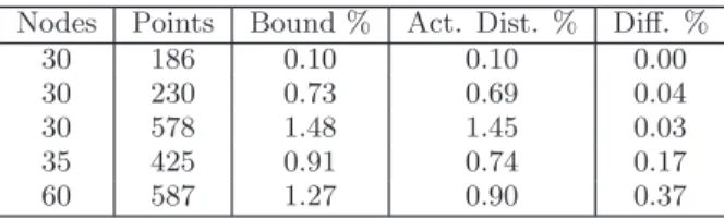
Table 2 compares the bounds with the actual distance from the optimal solution. We show the number of nodes

Nodes Points Bound % Act. Dist. % Diff. % 30 186 0.10 0.10 0.00 30 230 0.73 0.69 0.04 30 578 1.48 1.45 0.03 35 425 0.91 0.74 0.17 60 587 1.27 0.90 0.37

Table 2: Tightness of bounds

and points, the bound computed by our procedure, and the actual distance from the optimal solution. The last column shows the error in the bound (expressed in percentage of the coverable area), which is low, although it increases with the size of the deployment.

5. CONCLUSIONS

We have addressed the off-line problem of scheduling the wake-up times of a set of wireless nodes to maximize sens-ing coverage given a desired energy consumption level and lifetime. We employ partitioning techniques to recursively decompose an exponential problem and make it practical with current solvers. We have also shown how to compute upper bounds for the real optimal solution, and presented heuristic techniques to locally improve the final result.

Currently, we are considering the converse problem of maximizing the lifetime of the system given a desire average coverage. This could be set up as an independent prob-lem, or we can use our current formulation using a bisection procedure to identify the optimal point. The number of par-titions could progressively decreased in the bisection process to improve accuracy.

MILP formulations abound in the context of wireless sen-sor networks, and involve also problems such as routing topology creation [1] and energy-aware performance max-imization. We are currently exploring how to extend our

technique to these cases, which includes the creation of clus-ters on the basis of node connectivity. One problem that we need to address, for instance in the case of routing, is how to deal with dependencies between partitions which are not accounted for during the partitioning process itself. One solution would be to locally augment the partitions with a limited number of virtual nodes that model such dependen-cies, in the spirit of the “terminal propagation” technique [4]. The evaluation of bounds would have to be adapted accord-ingly.

6. REFERENCES

[1] J. N. Al-Karaki, R. Ul-Mustafa, and A. E. Kamal. Data aggregation in wireless sensor networks - exact and approximate algorithms. In IEEE Workshop on High Performance Switching and Routing (HPSR) 2004, Phoenix, Arizona, USA, April 2004. [2] A. Alfieri, A. Bianco, P. Brandimarte, and C. F.

Chiasserini. Maximizing system lifetime in wireless sensor networks. European Journal of Operational Research, 127(1):390–402, August 2007.

[3] M. Cardei, M. Thai, Y. Li, and W. Wu.

Energy-efficient target coverage in wireless sensor networks. In Proc. of INFOCOM, 2005.

[4] A. E. Dunlop and B. W. Kernighan. A procedure for placement of standard-cell VLSI circuits. IEEE Transactions on Computer-Aided Design of Integrated Circuits and Systems, 4(1):92–98, January 1985. [5] C. M. Fiduccia and R. M. Mattheyses. A linear time

heuristic for improving network partitions. In Proceedings of the 19th _{Design Automation}

Conference, pages 175–181, June 14-16, 1982. [6] C. Huang and Y. Tseng. The coverage problem in a

wireless sensor network. In Proc. of the 2nd_{ACM Int.}

Conf. on Wireless Sensor Networks and Applications (WSNA03), September 2003.

[7] H. Liu, X. Jia, P. Wan, C. Yi, S. Makki, and

N. Pissinou. Maximizing lifetime of sensor surveillance systems. IEEE/ACM Trans. on Networking,

15(2):334–345, 2007.

[8] MLPart. http://vlsicad.ucsd.edu/GSRC/ bookshelf/Slots/Partitioning/MLPart/.

[9] L. Palopoli, R. Passerone, G. P. Picco, A. L. Murphy, and A. Giusti. Maximizing sensing coverage in wireless sensor networks through optimal scattering of wake-up times. Technical Report DIT-07-048, DIT, University of Trento, July 2007.

[10] S. Slijepcevic and M. Potkonjak. Power efficient organization of wireless sensor networks. In Proc. of the IEEE Int. Conf. on Communications (ICC), June 2001.

[11] D. Tian and N. Georganas. A coverage-preserving node scheduling scheme for large wireless sensor networks. In First ACM Int. Wkshp. on Wireless Sensor networks and Applications (WSNA), 2002.