DISI - Via Sommarive 14 - 38123 Povo - Trento (Italy)
http://www.disi.unitn.it
COMPUTING MINIMAL MAPPINGS
BETWEEN LIGHTWEIGHT
ONTOLOGIES
Fausto Giunchiglia, Vincenzo Maltese,
Aliaksandr Autayeu
March 2010
Technical Report # DISI-10-027
Computing minimal mappings
between lightweight ontologies
1Fausto Giunchiglia, Vincenzo Maltese, Aliaksandr Autayeu
Dipartimento di Ingegneria e Scienza dell’Informazione (DISI) - Università di Trento {fausto, maltese, autayeu}@disi.unitn.it
Abstract. As a valid solution to the semantic heterogeneity problem, many
matching solutions have been proposed. Given two lightweight ontologies, we compute the minimal mapping, namely the subset of all possible correspond-ences, that we call mapping elements, between them such that i) all the others can be computed from them in time linear in the size of the input ontologies, and ii) none of them can be dropped without losing property i). We provide a formal definition of minimal mappings and define a time efficient computation algorithm which minimizes the number of comparisons between the nodes of the two input ontologies. The experimental results show a substantial improve-ment both in the computation time and in the number of mapping eleimprove-ments which need to be handled, for instance for validation, navigation and search.
Keywords: Interoperability, Ontology matching, lightweight ontologies,
mini-mal mappings
1 Introduction
Given any two graph-like structures, e.g., database and XML schemas, classifications, thesauri and ontologies, matching is usually identified as the problem of finding those nodes in the two structures which semantically correspond to one another. Any such pair of nodes, along with the semantic relationship holding between the two, is what we call a mapping element. In the last few years a lot of work has been done on this topic both in the digital libraries [15, 16, 17, 21, 23, 24, 25, 26, 29] and the computer science [2, 3, 4, 5, 6, 8, 9] communities.
We concentrate on lightweight ontologies (or formal classifications), as formally defined in [1, 7]. This must not be seen as a limitation. There are plenty of schemas in the world which can be translated, with almost no loss of information, into light-weight ontologies. For instance, thesauri, library classifications, file systems, email folder structures, web directories, business catalogues and so on. Lightweight ontolo-gies are well defined and pervasive. We focus on the problem of computing the
mini-mal mapping, namely the subset of all possible mapping elements such that i) all the
others can be computed from them in time linear in the size of the input graphs, and
1This paper is an integrated and extended version of two papers. The first was entitled
"Com-puting minimal mapping" and was presented at the 4th Workshop on Ontology Matching [22]; the second was entitled "Save up to 99% of your time in mapping validation" and was present-ed at the 9th International ODBASE Conference [34].
ii) none of them can be dropped without losing property i). The minimal mapping is the set of maximum size with no redundant elements. By concentrating on lightweight ontologies, we are able to identify specific redundancy patterns that are at the basis of what we define to be a minimal mapping. Such patterns are peculiar of lightweight ontologies and not of all ontologies in general. The main advantage of minimal map-pings is that they are the minimal amount of information that needs to be dealt with. Notice that this is a rather important feature as the number of possible mapping ele-ments can grow up to n*m with n and m being the size of the two input ontologies. Minimal mappings provide clear usability advantages. Many systems and correspond-ing interfaces, mostly graphical, have been provided for the management of mappcorrespond-ings but all of them hardly scale with the increasing number of nodes, and the resulting visualizations are rather messy [3]. Furthermore, the maintenance of smaller sets makes the work of the user much easier, faster and less error prone [11].
Our main contributions are a) a formal definition of minimal and, dually,
redun-dant mappings, b) evidence of the fact that the minimal mapping always exists and it
is unique and c) an algorithm to compute it. This algorithm has the following main features:
1. It can be proved to be correct and complete, in the sense that it always com-putes the minimal mapping;
2. It is very efficient as it minimizes the number of calls to the node matching function, namely to the function which computes the relation between two nodes. Notice that node matching in the general case amounts to logical rea-soning (i.e., SAT rearea-soning) [5], and it may require exponential time;
3. To compute the set of all correspondences between the two ontologies, it com-putes the mapping of maximum size (including the maximum number of re-dundant elements). This is done by maximally exploiting the information codi-fied in the graph of the lightweight ontologies in input. This, in turn, helps to avoid missing mapping elements due to pitfalls in the node matching func-tions, such as missing background knowledge [8].
As far as we know very little work has been done on the issue of computing mini-mal mappings. In general the computation of minimini-mal mappings can be seen as a spe-cific instance of the mapping inference problem [4]. Closer to our work, in [9, 10, 11] the authors use Distributed Description Logics (DDL) [12] to represent and reason about existing ontology mappings. They introduce a few debugging heuristics which remove mapping elements which are redundant or generate inconsistencies in a given set [10]. The main problem of this approach, as also recognized by the authors, is the complexity of DDL reasoning [11]. In our approach, by concentrating on lightweight ontologies, instead of pruning redundant elements, we directly compute the minimal set. Among other things, our approach allows minimizing the number of calls to the node matching functions.
The rest of the paper is organized as follows. Section 2 provides a motivating ex-ample and shows how we convert classifications into lightweight ontologies. Section 3 provides the definition for redundant and minimal mappings and it shows that the minimal set always exists and it is unique. Section 4 describes the algorithm while Section 5 evaluates it. Finally, Section 6 summarizes and concludes the paper.
2 Converting classifications into lightweight ontologies
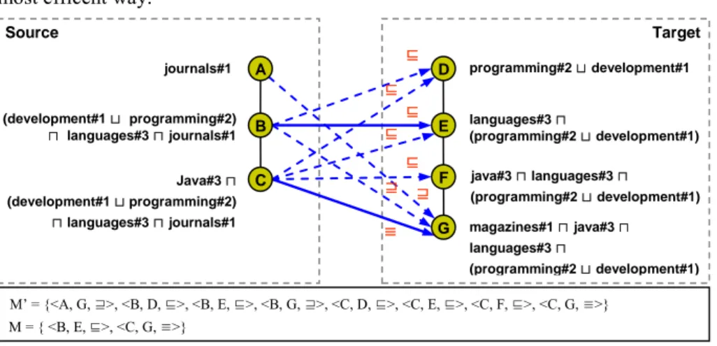
Classifications are perhaps the most natural tool humans use to organize information content. Information items are hierarchically arranged under topic nodes moving from general ones to more specific ones as long as we go deeper in the hierarchy. This atti-tude is well known in Knowledge Organization as the principle of organizing from the general to the specific [16], called synthetically the get-specific principle in [1, 7]. Consider the two fragments of classifications depicted in Fig. 1. They are designed to arrange more or less the same content, but from different perspectives. The second is a fragment taken from the Yahoo web directory2 (category Computers and Internet).
Fig. 1. Two classifications
Following the approach described in [1] and exploiting dedicated NLP techniques tuned to short phrases (for instance, as described in [13]), classifications can be con-verted, exactly or with a certain degree of approximation, into their formal alter-ego, namely into lightweight ontologies. Lightweight ontologies are acyclic graph struc-tures where each natural language node label is translated into a propositional De-scription Logic (DL) formula codifying the meaning of the node. Note that the formu-la associated to each node contains the formuformu-la of the node above to capture the fact that the meaning of each node is contextualized by the meaning of its ancestor nodes. As a consequence, the backbone structure of the resulting lightweight ontologies is represented by subsumption relations between nodes. The resulting formulas are re-ported in Fig. 2.
Here each string denotes a concept (such as journals#1) and the number at the end of the string denotes a specific concept constructed from a WordNet synset. Fig. 2 al-so reports the resulting mapping elements. We assume that each mapping element is associated with one of the following semantic relations: disjointness (⊥), equivalence (≡), more specific (⊑) and less specific (⊒), as computed for instance by semantic matching [5]. Notice that not all the mapping elements have the same semantic va-lence. For instance, B⊑D is a trivial logical consequence of B⊑E and E⊑D, and simi-larly for C⊑F and C≡G. We represent the elements in the minimal mapping using sol-id lines and redundant elements using dashed lines. M’ is the set of maximum size (including the maximum number of redundant elements) while M is the minimal set.
2http://dir.yahoo.com/ journals development and programming languages java programming and development languages java Classification (1) Classification (2) magazines A B C D E F G
The problem we address in the following is how to compute the minimal set in the most efficent way.
Fig. 2. The minimal and redundant mapping between two lightweight ontologies
3 Redundant and minimal mappings
Adapting the definition in [1] we define a lightweight ontology as follows:
Definition 1 (Lightweight ontology). A lightweight ontology O is a rooted tree
<N,E,LF> where:
a) N is a finite set of nodes; b) E is a set of edges on N;
c) LF is a finite set of labels expressed in a Propositional DL language such that for any node ni N, there is one and only one label liFLF;
d) li+1F ⊑ liF with ni being the parent of ni+1.
The superscript F is used to emphasize that labels are in a formal language. Fig. 2 above provides an example of (a fragment of) two lightweight ontologies.
We then define mapping elements as follows:
Definition 2 (Mapping element). Given two lightweight ontologies O1 and O2, a
mapping element m between them is a triple <n1, n2, R>, where:
a) n1N1 is a node in O1, called the source node;
b) n2N2 is a node in O2, called the target node;
c) R {⊥, ≡, ⊑, ⊒} is the strongest semantic relation holding between n1 and n2.
The partial order is such that disjointness is stronger than equivalence which, in turn, is stronger than subsumption (in both directions), and such that the two sub-sumption symbols are unordered. This is in order to return subsub-sumption only when equivalence does not hold or one of the two nodes being inconsistent (this latter case generating at the same time both a disjointness and a subsumption relation), and simi-larly for the order between disjointness and equivalence. Notice that under this order-ing there can be at most one mapporder-ing element between two nodes.
M’ = {<A, G, ⊒>, <B, D, ⊑>, <B, E, ⊑>, <B, G, ⊒>, <C, D, ⊑>, <C, E, ⊑>, <C, F, ⊑>, <C, G, ≡>} M = { <B, E, ⊑>, <C, G, ≡>} Source Target A B C D E F G ⊒ ⊒ ≡ ⊑ ⊑ ⊑ ⊑ ⊑
journals#1 programming#2 ⊔ development#1
languages#3 ⊓ (programming#2 ⊔ development#1) java#3 ⊓ languages#3 ⊓ (programming#2 ⊔ development#1) magazines#1 ⊓ java#3 ⊓ languages#3 ⊓ (programming#2 ⊔ development#1) (development#1 ⊔ programming#2) ⊓ languages#3 ⊓ journals#1 Java#3 ⊓ (development#1 ⊔ programming#2) ⊓ languages#3 ⊓ journals#1
The next step is to define the notion of redundancy. The key idea is that, given a mapping element <n1, n2, R>, a new mapping element <n1’, n2’, R’> is redundant with
respect to the first if the existence of the second can be asserted simply by looking at the relative positions of n1 with n1’, and n2 with n2’. In algorithmic terms, this means
that the second can be computed without running the time expensive node matching functions. We have identified four basic redundancy patterns as follows:
Fig. 3. Redundancy detection patterns
In Fig. 3, straight solid arrows represent minimal mapping elements, dashed arrows represent redundant mapping elements, and curves represent redundancy propagation. Let us discuss the rationale for each of the patterns:
Pattern (1): each mapping element <C, D, ⊑> is redundant w.r.t. <A, B, ⊑>. In fact, C is more specific than A which is more specific than B which is more specific than D. As a consequence, by transitivity C is more specific than D. Pattern (2): dual argument as in pattern (1).
Pattern (3): each mapping element <C, D, ⊥> is redundant w.r.t. <A, B, ⊥>. In fact, we know that A and B are disjoint, that C is more specific than A and that D is more specific than B. This implies that C and D are also disjoint.
Pattern (4): Pattern 4 is the combination of patterns (1) and (2).
In other words, the patterns are the way to capture logical inference from structural information, namely just by looking at the position of the nodes in the two trees. Note that they capture the logical inference w.r.t. one mapping element only. As we will show, this in turn allows computing the redundant elements in linear time (w.r.t. the size of the two ontologies) from the ones in the minimal set.
Fig. 4. Examples of non redundant mapping elements
A B C D (1) ⊑ ⊑ A B (2) C D ⊒ ⊒ A B C (3) D ⊥ C D E F (4) A B ≡ ≡ ⊥ ≡
Minimal mapping element
Redundancy propagation
Redundant mapping element
C D A ⊑ Car Automobile ≡ Auto ≡ C D B ⊑ A ⊑ ⊑ ⊑ Mammal Canine Animal Dog (a) (b)
Notice that patterns (1) and (2) are still valid in case we substitute subsumption with equivalence. However, in this case we cannot exclude the possibility that a stronger relation holds. A trivial example of where this is not the case is provided in Fig. 4 (a).
On the basis of the patterns and the considerations above we can define redundant elements as follows. Here path(n) is the path from the root to the node n.
Definition 3 (Redundant mapping element). Given two lightweight ontologies O1
and O2, a mapping M and a mapping element m’M with m’ = <C, D, R’> between
them, we say that m’ is redundant in M iff one of the following holds:
(1) If R’ is ⊑, ∃mM with m = <A, B, R> and m ≠ m’ such that R {⊑, ≡}, A path(C) and D path(B);
(2) If R’ is ⊒, ∃mM with m = <A, B, R> and m ≠ m’ such that R {⊒, ≡}, C path(A) and B path(D);
(3) If R’ is ⊥, ∃mM with m = <A, B, ⊥> and m ≠ m’ such that A path(C) and B path(D);
(4) If R’ is ≡, conditions (1) and (2) must be satisfied.
See how Definition 3 maps to the four patterns in Fig. 3. Fig. 2 provides examples of redundant elements. Definition 3 can be proved to capture all and only the cases of redundancy.
Theorem 1 (Redundancy, soundness and completeness). Given a mapping M between
two lightweight ontologies O1 and O2, a mapping element m’ M is logically
redun-dant w.r.t. another mapping element m M if and only if it satisfies one of the condi-tions of Definition 3.
The soundness argument is the rationale described for the patterns above. Com-pleteness can be shown by constructing the counterargument that we cannot have re-dundancy in the remaining cases. We can proceed by enumeration, negating each of the patterns, encoded one by one in the conditions appearing in the Definition 3. The complete proof is given in the appendix. Fig. 4 (b) provides an example of non redun-dancy which is based on pattern (1). It tells us that the existence of a correspondence between two nodes does not necessarily propagate to the two nodes below. For exam-ple we cannot derive that Canine ⊑ Dog from the set of axioms {Canine ⊑ Mammal,
Mammal ⊑ Animal, Dog ⊑ Animal}, and it would be wrong to do so.
Using the notion of redundancy, we formalize the minimal mapping as follows:
Definition 4 (Minimal mapping). Given two lightweight ontologies O1 and O2, we
say that a mapping M between them is minimal iff:
a) ∄mM such that m is redundant (minimality condition); b) ∄M’⊃M satisfying condition a) above (maximality condition). A mapping element is minimal if it belongs to the minimal mapping.
Note that conditions (a) and (b) ensure that the minimal set is the set of maximum size with no redundant elements. As an example, the set M in Fig. 2 is minimal. Comparing this mapping with M’ we can observe that all elements in the set M’ - M are redundant and that, therefore, there are no other supersets of M with the same properties. In effect, <A, G, ⊒> and <B, G, ⊒> are redundant w.r.t. <C, G, ≡> for pat-tern (2); <C, D, ⊑>, <C, E, ⊑> and <C, F, ⊑> are redundant w.r.t. <C, G, ≡> for pat-tern (1); <B, D, ⊑> is redundant w.r.t. <B, E, ⊑> for pattern (1). Note that M contains far less mapping elements w.r.t. M’.
As last observation, for any two given lightweight ontologies, the minimal map-ping always exists and it is unique. In fact, Definition 3 imposes a strict partial order over mapping elements. In other words, given two elements m and m’, m’ < m if and only if m’ is redundant w.r.t. m. Under the strict partial order above, the minimal mapping is the set of all the maximal elements of the partially ordered set.
Keeping in mind the patterns in Fig. 3, the minimal set can be efficiently computed using the following key intuitions:
1. Equivalence can be “opened” into two subsumption mapping elements of opposite direction;
2. Taking any two paths in the two ontologies, a minimal subsumption mapping element (in both directions of subsumption) is an element with the highest node in one path whose formula is subsumed by the formula of the lowest node in the other path;
3. Taking any two paths in the two ontologies, a minimal disjointness mapping element is the one with the highest nodes in both paths such that their formu-las satisfy disjointness.
4 Computing minimal and redundant mappings
The patterns described in the previous section allow us not only to identify minimal and redundant mapping elements, but they also suggest how to significantly reduce the amount of calls to the node matchers. By looking for instance at pattern (2) in Fig. 3, given a mapping element m = <A, B, ⊒> we know in advance that it is not neces-sary to compute the semantic relation holding between A and any descendant C in the sub-tree of B since we know in advance that it is ⊒. At the top level the algorithm is organized as follows:
Step 1, computing the minimal mapping modulo equivalence: compute the
set of disjointness and subsumption mapping elements which are minimal
modulo equivalence. By this we mean that they are minimal modulo
collaps-ing, whenever possible, two subsumption relations of opposite direction into a single equivalence mapping element;
Step 2, computing the minimal mapping: eliminate the redundant
subsump-tion mapping elements. In particular, collapse all the pairs of subsumpsubsump-tion el-ements (of opposite direction) between the same two nodes into a single equivalence element. This will result into the minimal mapping;
Step 3, computing the mapping of maximum size: compute the mapping of
this step the existence of a (redundant) element is computed as the result of the propagation of the elements in the minimal mapping. Notice that redundant equivalence mapping elements can be computed due to the propagation of minimal equivalence elements or of two minimal subsumption elements of opposite direction. However, it can be easily proved that in the latter case they correspond to two partially redundant equivalence elements, where a partially redundant equivalence element is an equivalence element where one direction is a redundant subsumption mapping element while the other is not.
The first two steps are performed at matching time, while the third is activated whenever the user wants to exploit the pre-computed mapping elements, e.g. for their visualization. The following three subsections analyze the three steps above in detail.
4.1 Step 1: Computing the minimal mapping modulo equivalence
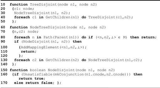
The minimal mapping is computed by a function TreeMatch whose pseudo-code is provided in Fig. 5. M is the minimal set, while T1 and T2 are the input lightweight ontologies. TreeMatch is crucially dependent on the two node matching functions
NodeDisjoint (Fig. 6) and NodeSubsumedBy (Fig. 7) which take two nodes n1 and
n2 and return a positive answer in case of disjointness and subsumption, or a negative answer if it is not the case or they are not able to establish it. Note that these two func-tions hide the heaviest computational costs. In particular, their computation time is exponential when the relation holds and exponential in the worst case, but possibly much faster, when the relation does not hold. The main motivation for this is that the node matching problem, in the general case, should be translated into disjointness or subsumption problem in propositional DL (see [5] for a detailed description).
10 node: struct of {cnode: wff; children: node[];} 20 T1,T2: tree of (node);
30 relation in {⊑, ⊒, ≡, ⊥};
40 element: struct of {source: node; target: node; rel: relation;}; 50 M: list of (element);
60 boolean direction;
70 function TreeMatch(tree T1, tree T2) 80 {TreeDisjoint(root(T1),root(T2)); 90 direction := true; 100 TreeSubsumedBy(root(T1),root(T2)); 110 direction := false; 120 TreeSubsumedBy(root(T2),root(T1)); 130 TreeEquiv(); 140 };
Fig. 5. Pseudo-code for the tree matching function
The goal, therefore, is to compute the minimal mapping by minimizing the calls to the node matching functions and, in particular minimizing the calls where the relation will turn out to hold. We achieve this purpose by processing both trees top down. To maximize the performance of the system, TreeMatch has therefore been built as the sequence of three function calls: the first call to TreeDisjoint (line 80) computes the minimal set of disjointness mapping elements, while the second and the third call to
two directions modulo equivalence (lines 90-120). Notice that in the second call,
TreeSubsumedBy is called with the input ontologies with swapped roles. The
varia-ble direction is used to change the direction of the subsumption. These three calls correspond to Step 1 above. They enforce patterns (1), (2) and (3). Line 130 in the pseudo code of TreeMatch implements Step 2 and it will be described in the next subsection. It enforces pattern (4), as the combination of patterns (1) and (2).
TreeDisjoint (Fig. 6) is a recursive function that finds all disjointness minimal
el-ements between the two sub-trees rooted in n1 and n2. Following the definition of re-dundancy, it basically searches for the first disjointness element along any pair of paths in the two input trees. Exploiting the nested recursion of NodeTreeDisjoint in-side TreeDisjoint, for any node n1 in T1 (traversed top down, depth first)
Node-TreeDisjoint visits all of T2, again top down, depth first. NodeNode-TreeDisjoint (called
at line 30, starting at line 60) keeps fixed the source node n1 and iterates on the whole target sub-tree below n2 till, for each path, the highest disjointness element, if any, is found. Any such disjointness element is added only if minimal (lines 90-120). The condition at line 80 is necessary and sufficient for redundancy. The idea here is to ex-ploit the fact that any two nodes below two nodes involved in a disjointness mapping element are part of a redundant element and, therefore, to stop the recursion. This saves a lot of time expensive calls (n*m calls with n and m the number of the nodes in the two sub-trees). Notice that this check needs to be performed on the full path. At this purpose, NodeDisjoint checks whether the formula obtained by the conjunction of the formulas associated to the nodes n1 and n2 is unsatisfiable (lines 150-170).
10 function TreeDisjoint(node n1, node n2) 20 {c1: node;
30 NodeTreeDisjoint(n1, n2);
40 foreach c1 in GetChildren(n1) do TreeDisjoint(c1,n2); 50 };
60 function NodeTreeDisjoint(node n1, node n2) 70 {n,c2: node;
80 foreach n in Path(Parent(n1)) do if (<n,n2,⊥> M) then return;
90 if (NodeDisjoint(n1, n2)) then 100 {AddMappingElement(<n1,n2,⊥>); 110 return;
120 };
130 foreach c2 in GetChildren(n2) do NodeTreeDisjoint(n1,c2); 140 };
150 function boolean NodeDisjoint(node n1, node n2)
160 {if (Unsatisfiable(mkConjunction(n1.cnode,n2.cnode))) then return true;
170 else return false; };
Fig. 6. Pseudo-code for the TreeDisjoint function
TreeSubsumedBy (Fig. 7) recursively finds all minimal mapping elements where
the strongest relation between the nodes is ⊑ (or dually, ⊒ in the second call; in the following we will concentrate only on the first call). Notice that TreeSubsumedBy assumes that the minimal disjointness elements are already computed. As a conse-quence, at line 30 it checks whether the mapping element between the nodes n1 and n2 is already in the minimal set. If this is the case it stops the recursion. This allows
computing the stronger disjointness relation rather than subsumption when both hold (namely with an inconsistent node). Given n2, lines 40-50 implement a depth first re-cursion in the first tree till a subsumption is found. The test for subsumption is per-formed by function NodeSubsumedBy that checks whether the formula obtained by the conjunction of the formulas associated to the node n1 and the negation of the for-mula for n2 is unsatisfiable (lines 170-190). Lines 60-140 implement what happens after the first subsumption is found. The key idea is that, after finding the first sub-sumption, TreeSubsumedBy keeps recursing down the second tree till it finds the last subsumption. When this happens, the resulting mapping element is added to the min-imal mapping (line 100). Notice that both NodeDisjoint and NodeSubsumedBy call the function Unsatisfiable which embeds a call to a SAT solver.
10 function boolean TreeSubsumedBy(node n1, node n2) 20 {c1,c2: node; LastNodeFound: boolean;
30 if (<n1,n2,⊥> M) then return false;
40 if (!NodeSubsumedBy(n1, n2)) then
50 foreach c1 in GetChildren(n1) do TreeSubsumedBy(c1,n2); 60 else
70 {LastNodeFound := false;
80 foreach c2 in GetChildren(n2) do
90 if (TreeSubsumedBy(n1,c2)) then LastNodeFound := true; 100 if (!LastNodeFound) then AddSubsumptionMappingElement(n1,n2); 120 return true;
140 };
150 return false; 160 };
170 function boolean NodeSubsumedBy(node n1, node n2)
180 {if (Unsatisfiable(mkConjunction(n1.cnode,negate(n2.cnode)))) then return true;
190 else return false; };
200 function AddSubsumptionMappingElement(node n1, node n2) 210 {if (direction) then AddMappingElement(<n1,n2,⊑>); 220 else AddMappingElement(<n2,n1,⊒>); };
Fig. 7. Pseudo-code for the TreeSubsumedBy function
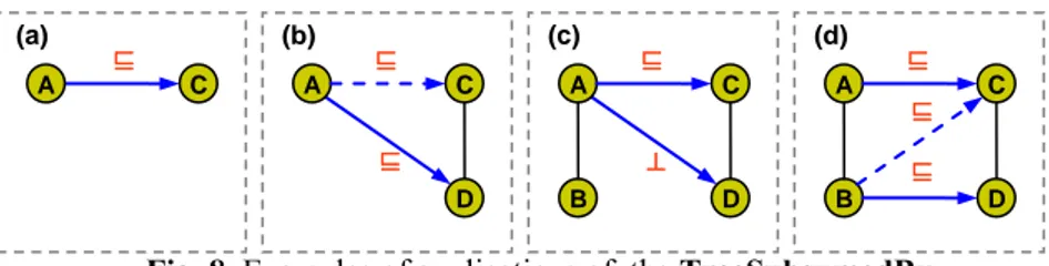
To fully understand TreeSubsumedBy, the reader should check what happens in the four situations in Fig. 8. In case (a) the first iteration of the TreeSubsumedBy finds a subsumption between A and C. Since C has no children, it skips lines 80-90 and directly adds the mapping element <A, C, ⊑> to the minimal set (line 100). In case (b), since there is a child D of C the algorithm iterates on the pair A-D (lines 80-90) finding a subsumption between them. Since there are no other nodes under D, it adds the mapping element <A, D, ⊑> to the minimal set and returns true. Therefore LastNodeFound is set to true (line 90) and the mapping element between the pair A-C is recognized as redundant. Case (c) is similar. The difference is that
TreeSub-sumedBy will return false when checking the pair A-D (line 30) - thanks to previous
computation of minimal disjointness mapping elements - and therefore the mapping element <A, C, ⊑> is recognized as minimal. In case (d) the algorithm iterates after the second subsumption mapping element is identified. It first checks the pair A-C and iterates on A-D concluding that subsumption does not hold between them (line
40). Therefore, it recursively calls TreeSubsumedBy between B and D. In fact, since <A, C, ⊑> will be recognized as minimal, it is not worth checking <B, C, ⊑> because of pattern (1). As a consequence the mapping element <B, D, ⊑> is recognized as minimal together with <A, C, ⊑>.
Fig. 8. Examples of applications of the TreeSubsumedBy
Five observations about the TreeMatch function. The first is that, even if, overall,
TreeMatch implements three loops instead of one, the wasted (linear) time is largely
counterbalanced by the exponential time saved by avoiding a lot of useless calls to the SAT solver. The second is that, when the input trees T1 and T2 are two nodes,
Tree-Match behaves as a node matching function which returns the semantic relation
hold-ing between the input nodes. The third is that the call to TreeDisjoint before the two calls to TreeSubsumedBy allows us to implement the partial order on relations de-fined in the previous section. In particular it allows returning only a disjointness map-ping element when both disjointness and subsumption hold. The fourth is the fact that skipping (in the body of the TreeDisjoint) the two sub-trees where disjointness holds is what allows not only implementing the partial order (see the previous observation) but also saving a lot of useless calls to the node matching functions. The fifth and last observation is that the implementation of TreeMatch crucially depends on the fact that the minimal elements of the two directions of subsumption and disjointness can be computed independently (modulo inconsistencies).
4.2 Step 2: Computing the minimal mapping
The output of Step 1 is the set of all disjointness and subsumption mapping elements which are minimal modulo equivalence. The final step towards computing the mini-mal mapping is that of collapsing any two subsumption relations, in the two direc-tions, holding between the same two nodes into a single equivalence relation. The key point is that equivalence is in the minimal set only if both subsumptions are in the minimal set. We have three possible situations:
1. None of the two subsumptions is minimal (in the sense that it has not been computed as minimal in Step 1): nothing changes and neither subsumption nor equivalence is memorized as minimal;
2. Only one of the two subsumptions is minimal while the other is not minimal (again according to Step 1): this case is solved by keeping only the subsump-tion mapping as minimal. Of course, during Step 3 (see below) the necessary computations will have to be done in order to show to the user the existence of an equivalence relation between the two nodes;
C A ⊑ D C A ⊑ (a) (b) ⊑ B D C A ⊑ (c) ⊥ B D C A ⊑ (d) ⊑ ⊑
3. Both subsumptions are minimal (according to Step 1): in this case the two subsumptions can be deleted and substituted with a single equivalence ele-ment. This implements the fact that pattern (4) is exactly the combination of the patterns (1) and (2).
Note that Step 2 can be computed very easily in time linear with the number of mapping elements output of Step 1: it is sufficient to check for all the subsumption el-ements of opposite direction between the same two nodes and to substitute them with an equivalence element. This is performed by function TreeEquiv in Fig. 5.
4.3 Step 3: Computing the mapping of maximum size
We concentrate on the following problem: given two lightweight ontologies T1 and T2 and the minimal mapping M compute the mapping element between two nodes n1 in T1 and n2 in T2 or the fact that no element can be computed given the current available background knowledge. Other problems are trivial variations of this one. The corresponding pseudo-code is given in Fig. 9.
10 function mapping ComputeMappingElement(node n1, node n2) 20 {isLG, isMG: boolean;
30 if ((<n1,n2,⊥> ∈ M) || IsRedundant(<n1,n2,⊥>)) then return <n1,n2,⊥>; 40 if (<n1,n2,≡> ∈ M) then return <n1,n2,≡>;
50 if ((<n1,n2,⊑> ∈ M) || IsRedundant(<n1,n2,⊑>)) then isLG := true; 60 if ((<n1,n2,⊒> ∈ M) || IsRedundant(<n1,n2,⊒>)) then isMG := true; 70 if (isLG && isMG) then return <n1,n2,≡>;
80 if (isLG) then return <n1,n2,⊑>; 90 if (isMG) then return <n1,n2,⊒>; 100 return NULL;
110 };
120 function boolean IsRedundant(mapping <n1,n2,R>) 130 {switch (R)
140 {case ⊑: if (VerifyCondition1(n1,n2)) then return true; break; 150 case ⊒: if (VerifyCondition2(n1,n2)) then return true; break; 160 case ⊥: if (VerifyCondition3(n1,n2)) then return true; break; 170 case ≡: if (VerifyCondition1(n1,n2) &&
VerifyCondition2(n1,n2)) then return true;
180 };
190 return false; 200 };
210 function boolean VerifyCondition1(node n1, node n2) 220 {c1,c2: node;
230 foreach c1 in Path(n1) do 240 foreach c2 in SubTree(n2) do
250 if ((<c1,c2,⊑> ∈ M) || (<c1,c2,≡> ∈ M)) then return true; 260 return false;
270 };
ComputeMappingElement is structurally very similar to the NodeMatch function
described in [5], modulo the key difference that no calls to SAT are needed.
Com-puteMappingElement always returns the mapping element with strongest relation.
More in detail, a mapping element is returned by the algorithm either in the case it is in the minimal set or it is redundant w.r.t. an element in the minimal set. The check is performed according to the partial order enforced on the semantic relations, i.e. at line 30 for ⊥, 40 for ≡, 50 for ⊑ and 60 for ⊒, where the first condition checks for the presence of the mapping element in the minimal set and the second for redundancy. Note that if both ⊑ and ⊒ hold, equivalence is returned (line 80). The test for redun-dancy performed by IsRedundant reflects the definition of redunredun-dancy provided in Section 3 above. We provide only the code which does the check for the first pattern; the others are analogous. Given for example a mapping element <n1, n2, ⊑>, condi-tion 1 is verified by checking (line 250) whether in M there is an element <c1, c2, ⊑> or <c1, c2, ≡> with c1 ancestor of n1 (c1 is taken from the path of n1, line 230) and c2 descendant of n2 (c2 is taken from the sub-tree of n2, line 240). Notice that
Com-puteMappingElement calls IsRedundant at most three times and, therefore, its
computation time is linear with the number of mapping elements in M.
5 Evaluation
The algorithm presented in the previous section has been implemented by taking the node matching routines of the state of the art matcher S-Match [5] and by changing the way the tree structure is matched. We call the new matcher MinSMatch. The evaluation has been performed by directly comparing the results of MinSMatch and S-Match on several real-world datasets. All tests have been performed on a Pentium D 3.40GHz with 2GB of RAM running Windows XP SP3 operating system with no additional applications running except the matching system. Both systems were lim-ited to allocating no more than 1GB of RAM. The tuning parameters were set to the default values. The selected datasets had been already used in previous evaluations, see [14, 31]. Some of these datasets can be found at the Ontology Alignment Evalua-tion Initiative (OAEI) web site3. The first two datasets describe courses and will be
called Cornell and Washington, respectively. The second two come from the arts do-main and will be referred to as Topia and Icon, respectively. The third two datasets have been extracted from the Looksmart, Google and Yahoo! directories and will be referred to as Source and Target. The fourth two datasets contain portions of the two business directories eCl@ss4 and UNSPSC5 and will be referred to as Eclass and
Un-spsc. Table 1 describes some indicators of the complexity of these datasets.
Consider Table 2. The reduction in the last column is calculated as (1 - m/t), where m is the number of elements in the minimal set and t is the total number of elements in the mapping of maximum size, as computed by MinSMatch. As it can be easily no-ticed, we have a significant reduction, in the range 68-96%.
3 http://oaei.ontologymatching.org/2006/directory/
4 http://www.eclass-online.com/
# Dataset pair Node count Max depth Average branching factor 1 Cornell/Washington 34/39 3/3 5.50/4.75 2 Topia/Icon 542/999 2/9 8.19/3.66 3 Source/Target 2857/6628 11/15 2.04/1.94 4 Eclass/Unspsc 3358/5293 4/4 3.18/9.09
Table 1. Complexity of the datasets
The second interesting observation is that in Table 2, in the last two experiments, the number of total mapping elements computed by MinSMatch is slightly higher (compare the second and the third column). This is due to the fact that in the presence of one of the patterns, MinSMatch directly infers the existence of a mapping element without testing it. This allows MinSMacth, differently from S-Match, to reduce miss-ing elements because of failures of the node matchmiss-ing functions (because of lack of background knowledge [8]). One such example from our experiments is reported be-low (directories Source and Target):
\Top\Computers\Internet\Broadcasting\Video Shows
\Top\Computing\Internet\Fun & Games\Audio & Video\Movies
We have a minimal mapping element which states that Video Shows ⊒ Movies. The element generated by this minimal one, which is captured by MinSMatch and missed by S-Match (because of the lack of background knowledge about the relation between ‘Broadcasting’ and ‘Movies’) states that Broadcasting ⊒ Movies.
S-Match MinSMatch # Total mapping elements (t) Total mapping elements (t) Minimal mapping elements (m) Reduction, % 1 223 223 36 83.86 2 5491 5491 243 95.57 3 282638 282648 30956 89.05 4 39590 39818 12754 67.97
Table 2. Mapping sizes.
To conclude our analysis, Table 3 shows the reduction in computation time and calls to SAT. As it can be noticed, the time reductions are substantial, in the range 16% - 59%, but where the smallest savings are for very small ontologies. In principle, the deeper the ontologies the more we should save. The interested reader can refer to [5, 14] for a detailed qualitative and performance evaluation of S-Match w.r.t. other state of the art matching algorithms.
Run Time, ms SAT calls # S-Match Min S-Match Reduction, % S-Match Min S-Match Reduction, % 1 472 397 15.88 3978 2273 42.86 2 141040 67125 52.40 1624374 616371 62.05 3 3593058 1847252 48.58 56808588 19246095 66.12 4 6440952 2642064 58.98 53321682 17961866 66.31
Table 3. Run time and SAT problems.
These results are confirmed by a recent experiment we conducted in matching NALT with LCSH [28] that are much deeper in structure (15 and 25 levels,
respec-tively). We executed MinSMatch on a selection of the branches which turned out to have a high percentage of semantically enrichable nodes, i.e. nodes whose labels could be parsed with success by our NLP pipeline. See Table 3 for details. Table 4 shows evaluation details about conducted experiments in terms of the branches which are matched, the number of elements in the mapping of maximum size (obtained by propagation from the elements in the minimal mapping), the number of elements in the minimal mapping and the percentage of reduction in the size of the minimal set w.r.t. the size of the mapping of maximum size.
Id Source Branch
Number of nodes
Enriched nodes
A NALT Chemistry and Physics 3944 97%
B NALT Natural Resources, Earth and Environmental Sciences 1546 96%
C LCSH Chemical Elements 1161 97%
D LCSH Chemicals 1372 93%
E LCSH Management 1137 91%
F LCSH Natural resources 1775 74%
Table 3. NALT and LCSH branches matched
Matching experiment maximum size Mapping of Minimal mapping Reduction
A
vs. C
Mapping elements found 17716 7541 57,43%
Disjointness 8367 692 91,73% Equivalence 0 0 --- more general 0 0 --- more specific 9349 6849 26,74%
A
vs. D
Mapping elements found 139121 994 99,29%
Disjointness 121511 754 99,38% Equivalence 0 0 --- more general 0 0 --- more specific 17610 240 98,64%
A
vs. E
Mapping elements found 9579 1254 86,91%
Disjointness 9579 1254 86,91% Equivalence 0 0 --- more general 0 0 --- more specific 0 0 ---
B
vs. F
Mapping elements found 27191 1232 95,47%
Disjointness 21352 1141 94,66%
Equivalence 24 1 95,83%
more general 2808 30 98,93%
more specific 3007 60 98,00%
We ran MinSMatch both between branches with an evident overlap in the topic (i.e. A vs. C and D, B vs. F) and between clearly unrelated branches (i.e. A vs. E). As expected, in the latter case we obtained only disjointness relations. This demonstrates that the tool is able to provide clear hints of places in which it is not worth to look at in case of search and navigation. All experiments confirm that the minimal mapping contains significantly less elements w.r.t. the mapping of maximum size (from 57% to 99%). Experiments also show that exact equivalence is quite rare. We found just 24 equivalences, and only one in a minimal mapping. This phenomenon has been ob-served also in other projects, for instance in Renardus [23] and CARMEN6.
Yet it is clear that, even if faster, automatic approaches require manual validation and augmentation of computed mappings (see for instance [27], which also describes a tool that supports this task). This is exactly where minimal mappings can be of great help. In fact, regardless the quality of the mapping returned by the algorithm, during the validation phase we can concentrate on the elements in the minimal mapping, a very small portion of the complete mapping, i.e. the mapping of maximum size. This makes manual validation much easier, faster, and less error-prone. In [34] we give concrete suggestions on how to effectively conduct the validation process.
We also conducted several experiments (described extensively in [32]) to study the differences between precision and recall measures when comparing the minimized (the mapping obtained by removing redundant correspondences) and maximized (the mapping obtained by adding all the redundant correspondences) versions of the gold-en standards with the minimized and maximized versions of the mapping returned by S-Match [5]. We used three different golden standards [33] already used in several evaluations. The first two datasets (101 and 304) come from OAEI; the two ontolo-gies describe publications, contain few nodes and corresponding golden standard is exhaustive. It only contains equivalence correspondences. The second (Topia and Icon) and third (Source and Target) pairs are described in Table 1.
Dataset pair Precision, % Recall, % min norm max min norm max 101/304 32.47 9.75 69.67 86.21 93.10 92.79 Topia/Icon 16.87 4.86 45.42 10.73 20.00 42.11 Source/Target 74.88 52.03 48.40 10.35 40.74 53.30
Table 5. Precision and Recall for minimized, normal and maximized sets.
Table 5 shows precision and recall figures obtained from the comparison of the minimized mapping with the minimized golden standards (min), the original mapping with the original golden standards (norm) and the maximized mapping with the max-imized golden standards (max) respectively. For what said above, the max columns provide the most accurate results. As it can be noted from the measures obtained comparing the maximized versions with the original versions, the performance of the S-Match algorithm is on average better than expected (with the exception of the preci-sion figure of the Source/Target experiment). More in general, the quality of the map-ping is a function of the quantity and quality of the available background knowledge. We are currently developing new methodologies for its construction [35].
6 Conclusions
In this paper we have provided a definition and a fast algorithm for the computa-tion of the minimal mapping between two lightweight ontologies. The evaluacomputa-tion shows a substantial improvement in the (much lower) computation time, in the (much lower) number of elements which need to be stored and handled and in the (higher) total number of mapping elements which are computed. As part of the evaluation we have presented the results of a matching experiment we conducted between two large scale knowledge organization systems: NALT and LCSH. They confirm that the min-imal mapping always contains a very little portion of the overall number of corre-spondences between the two ontologies; this makes manual validation much easier, up to two orders of magnitude faster, and less error-prone.
Finally, we have shown that to obtain more accurate evaluations one should max-imize both the golden standard and the matching result. Experiments show that for in-stance the state of the art matcher S-Match performs on average better than expected.
As future work we plan to explore the possibility to extend the notion of minimal mapping from lightweight ontologies to generic ontologies.
References
1. F. Giunchiglia, M. Marchese, I. Zaihrayeu, 2006. Encoding Classifications into Light-weight Ontologies. Journal of Data Semantics 8, pp. 57-81.
2. P. Shvaiko, J. Euzenat, 2007. Ontology Matching. Springer-Verlag New York, Inc. Secau-cus, NJ, USA.
3. P. Shvaiko, J. Euzenat, 2008. Ten Challenges for Ontology Matching. In Proc. of the 7th Int. Conference on Ontologies, Databases, and Applications of Semantics (ODBASE). 4. J. Madhavan, P. A. Bernstein, P. Domingos, A. Y. Halevy, 2002. Representing and
Rea-soning about Mappings between Domain Models. At the 18th National Conference on Arti-ficial Intelligence (AAAI 2002).
5. F. Giunchiglia, M. Yatskevich, P. Shvaiko, 2007. Semantic Matching: algorithms and im-plementation. Journal on Data Semantics, IX, 2007.
6. C. Caracciolo, J. Euzenat, L. Hollink, R. Ichise, A. Isaac, V. Malaisé, C. Meilicke, J. Pane, P. Shvaiko, 2008. First results of the Ontology Alignment Evaluation Initiative 2008. 7. F. Giunchiglia, I. Zaihrayeu, 2007. Lightweight Ontologies. In The Encyclopedia of
Data-base Systems, to appear. Springer, 2008.
8. F. Giunchiglia, P. Shvaiko, M. Yatskevich, 2006. Discovering missing background knowledge in ontology matching. In Proc. of the 17th European Conference on Artificial Intelligence (ECAI 2006), pp. 382–386.
9. H. Stuckenschmidt, L. Serafini, H. Wache, 2006. Reasoning about Ontology Mappings. In Proc. of the ECAI-06 Workshop on Contextual Representation and Reasoning.
10. C. Meilicke, H. Stuckenschmidt, A. Tamilin, 2006. Improving automatically created map-pings using logical reasoning. In Proc. of the 1st International Workshop on Ontology Matching OM-2006, CEUR Workshop Proceedings Vol. 225.
11. C. Meilicke, H. Stuckenschmidt, A. Tamilin, 2008. Reasoning support for mapping revi-sion. Journal of Logic and Computation, 2008.
12. A. Borgida, L. Serafini. Distributed Description Logics: Assimilating Information from Peer Sources. Journal on Data Semantics pp. 153-184.
13. I. Zaihrayeu, L. Sun, F. Giunchiglia, W. Pan, Q. Ju, M. Chi, and X. Huang, 2007. From
web directories to ontologies: Natural language processing challenges. In 6th International
14. P. Avesani, F. Giunchiglia and M. Yatskevich, 2005. A Large Scale Taxonomy Mapping Evaluation. In Proc. of International Semantic Web Conference (ISWC 2005), pp. 67-81. 15. M. L. Zeng, L. M. Chan, 2004. Trends and Issues in Establishing Interoperability Among
Knowledge Organization Systems. Journal of the American Society for Information Sci-ence and Technology, 55(5) pp. 377–395.
16. L. Kovács. A. Micsik, 2007. Extending Semantic Matching Towards Digital Library Con-texts. Proc. of the 11th European Conference on Digital Libraries (ECDL), pp. 285-296. 17. B. Marshall, T. Madhusudan, 2004. Element matching in concept maps. In Proc. of the 4th
ACM/IEEE-CS Joint Conference on Digital Libraries (JCDL 2004), pp.186-187.
18. B. Hjørland, 2008. What is Knowledge Organization (KO)?. Knowledge Organization. In-ternational Journal devoted to Concept Theory, Classification, Indexing and Knowledge Representation 35(2/3) pp. 86-101.
19. D. Soergel, 1972. A Universal Source Thesaurus as a Classification Generator. Journal of the American Society for Information Science 23(5), pp. 299–305.
20. D. Vizine-Goetz, C. Hickey, A. Houghton, and R. Thompson. 2004. Vocabulary Mapping for Terminology Services. Journal of Digital Information, Volume 4, Issue 4.
21. M. Doerr, 2001. Semantic Problems of Thesaurus Mapping. Journal of Digital Information, Volume 1, Issue 8.
22. F. Giunchiglia, V. Maltese, A. Autayeu, 2009. Computing minimal mappings. At the 4th Ontology Matching Workshop as part of the ISWC 2009.
23. T. Koch, H. Neuroth, M. Day, 2003. Renardus: Cross-browsing European subject gateways via a common classification system (DDC). In I.C. McIlwaine (Ed.), Subject retrieval in a networked environment. In Proc. of the IFLA satellite meeting held in Dublin pp. 25–33. 24. D. Nicholson, A. Dawson, A. Shiri, 2006. HILT: A pilot terminology mapping service with
a DDC spine. Cataloging & Classification Quarterly, 42 (3/4). pp. 187-200.
25. C. Whitehead, 1990. Mapping LCSH into Thesauri: the AAT Model. In Beyond the Book: Extending MARC for Subject Access, pp. 81.
26. E. O'Neill, L. Chan, 2003. FAST (Faceted Application for Subject Technology): A Simpli-fied LCSH-based Vocabulary. World Library and Information Congress: 69th IFLA Gen-eral Conference and Council, 1-9 August, Berlin.
27. S. Falconer, M. Storey, 2007. A cognitive support framework for ontology mapping. In Proc. of ISWC/ASWC, 2007.
28. F. Giunchiglia, D. Soergel, V. Maltese, A. Bertacco, 2009. Mapping large-scale Knowledge Organization Systems. In Proc. of the 2nd International Conference on the Se-mantic Web and Digital Libraries (ICSD), 2009.
29. B. Lauser, G. Johannsen, C. Caracciolo, J. Keizer, W. R. van Hage, P. Mayr, 2008. Com-paring human and automatic thesaurus mapping approaches in the agricultural domain. In Proc. Int’l Conf. on Dublin Core and Metadata Applications.
30. J. David, J. Euzenat, 2008. On Fixing Semantic Alignment Evaluation Measures. In Proc. of the Third International Workshop on Ontology Matching.
31. F. Giunchiglia, M. Yatskevich, P. Avesani, P. Shvaiko, 2008. A Large Dataset for the Evaluation of Ontology Matching Systems. The Knowledge Engineering Review Journal, 24(2), pp. 137-157.
32. A. Autayeu, V. Maltese, P. Andrews, 2010. Recommendations for Better Quality Ontology Matching Evaluations. In Proc. of the 2nd AISB Workshop on Matching and Meaning. 33. A. Autayeu, F. Giunchiglia, P. Andrews, Q. Ju, 2009. Lightweight Parsing of Natural
Lan-guage Metadata. In Proc. of the First Natural LanLan-guage Processing for Digital Libraries Workshop.
34. V. Maltese, F. Giunchiglia, A. Autayeu, 2010. Save up to 99% of your time in mapping validation. In Proc. of the 9th International ODBASE conference, 2010.
35. B. Dutta, F. Giunchiglia, V. Maltese, 2011. A facet-based methodology for geo-spatial modelling. In Proc. of GEOS, 6631, pp. 133–150.
Appendix: proofs of the theorems
Theorem 1 (Redundancy, soundness and completeness). Given a mapping M between
two lightweight ontologies O1 and O2, a mapping element m’ M is logically
redun-dant w.r.t. another mapping element m M if and only if it satisfies one of the condi-tions of Definition 3.
Proof:
Soundness: The argumentation provided in section 3 as a rationale for the patterns
al-ready provides a full demonstration for soundness.
Completeness: We can demonstrate the completeness by showing that we cannot have
redundancy (w.r.t. another mapping element) in the cases which do not fall in the conditions listed in Definition 3. We proceed by enumeration, negating each of the conditions. There are some trivial cases we can exclude in advance:
Fig. 10. Some trivial cases which do not fall in the redundancy patterns
- The trivial case in which m’ is the only mapping element between the lightweight ontologies. See Fig. 10 (a);
- Incomparable symbols. The only cases of dependency across symbols are cap-tured by conditions (1) and (2) in Definition 3, where equivalence can be used to derive the redundancy of a more or less specific mapping element. This is due to the fact that equivalence is exactly the combination of more and less specific. No other symbols can be expressed in terms of the others. This means for instance that we cannot establish implications between an element with more specific and one with disjointness. In Fig. 10 (b) the two elements do not influence each other; - All the cases of inconsistent nodes. See for instance Fig. 10 (c). If we assume the
element <A, B, ⊑> to be correct, then according to pattern (1) the mapping ele-ment between C and D should be <C, D, ⊑>. However, in case of inconsistent nodes the stronger semantic relation ⊥ holds. The algorithm presented in section 4 correctly returns ⊥ in these cases;
- Cases of underestimated strength not covered by the previous cases, namely the cases in which equivalence holds instead of the (weaker) subsumption. Look for instance at Fig. 10 (d). The two subsumptions in <A, B, ⊑> and <E, F, ⊑> must be equivalences. As a consequence, <C, D, ≡> is redundant for pattern (4). In fact, the chain of subsumptions E ⊑ … ⊑ C ⊑ … ⊑ A ⊑ B ⊑ … ⊑ D ⊑ … ⊑ F allows
to conclude that E ⊑ F holds and therefore E ≡ F. Symmetrically, we can
con-C D E F (d) A B ≡ ⊑ ⊒ A B C D ⊥ ⊑ (c) A B ⊥ ⊑ (b) C A B (a) ⊥
clude that A ≡ B. Note that the mapping elements <A, B, ⊑> and <E, F, ⊒> are minimal. We identify the strongest relations by propagation (at step 3 of the pro-posed algorithm, as described in section 4).
We refer to all the other cases as the meaningful cases.
Condition (1): its negation is when R ≠ “⊑” or A path(C) or D path(B). The cases in which R = “⊑” are shown in Fig. 11. For each case, the provided rationale shows that available axioms cannot be used to derive C ⊑ D from A ⊑ B. The remaining
meaningful cases, namely only when R = “≡”, are similar.
A path(C) D path(B) Rationale
(a) NO YES C ⊑ … ⊑ A, D ⊑ … ⊑ B, A ⊑ B cannot derive C ⊑ D (b) YES NO A ⊑ … ⊑ C, B ⊑ … ⊑ D, A ⊑ B cannot derive C ⊑ D (c) YES YES A ⊑ … ⊑ C, D ⊑ … ⊑ B, A ⊑ B cannot derive C ⊑ D
Fig. 11. Completeness of condition (1)
Condition (2): it is the dual of condition (1).
Condition (3): its negation is when R ≠ “⊥”or A path(C) or B path(D). The cases in which R = “⊥” are shown in Fig. 12. For each case, the provided rationale shows that available axioms cannot be used to derive C ⊥ D from A ⊥ B. There are no
meaningful cases for R ≠ “⊥”.
A path(C) B path(D) Rationale
(a) NO YES C ⊑ … ⊑ A, B ⊑ … ⊑ D, A ⊥ B cannot derive C ⊥ D (b) YES NO A ⊑ … ⊑ C, D ⊑ … ⊑ B, A ⊥ B cannot derive C ⊥ D (c) YES YES A ⊑ … ⊑ C, D ⊑ … ⊑ B, A ⊥ B cannot derive C ⊥ D
Fig. 12. Completeness of condition (3)
C D B ⊑ (a) A ⊑ ⊑ ⊑ ⊑ A B (c) C D ⊑ ⊑ ⊑ ⊑ A B D ⊑ (b) C ⊑ ⊑ C B D ⊥ (a) A ⊥ ⊑ ⊑ ⊑ A B D (c) C ⊑ ⊑ A D B (b) C ⊑ ⊥ ⊥ ⊥ ⊥
Condition (4): it can be easily noted from Fig. 3 that the redundant elements identified by pattern (4) are exactly all the mapping elements m’ = <C, D, ≡> with source C and target D respectively between (or the same of) the source node and target node of two different mapping elements m = <A, B, ≡> and m’’ = <E, F, ≡>. This configuration allows to derive from m and m’’ the subsumptions in the two directions which amount to the equivalence. The negation of condition 4 is when R ≠ “≡”in m or m’’ or A path(C) or D path(B) or C path(E) or F path(D). In almost all the cases (14 over 15) in which R = “≡” we just move the source C or the target D outside these ranges. For sake of space we show only some of such cases in Fig. 13. The rationale provided for cases (a) and (b) shows that we cannot derive C ≡ D from A ≡ B and E ≡ F. The only exception (the remaining 1 case over 15), represented by case (c), is
when A path(C) and D path(B) and C path(E) and F path(D). This case however is covered by condition 4 by inverting the role of m and m’’. The remaining cases, namely when R ≠ “≡” in m or m’’, are not meaningful.
A path(C) D path(B) C path(E) F path(D) Rationale
(a) NO NO NO YES
E ⊑ … ⊑ C, C ⊑ … ⊑ A, B ⊑ … ⊑ F, F ⊑ … ⊑ D, A ≡ B and E ≡ F cannot
derive C ≡ D (we can only derive C ⊑ D).
(b) NO NO YES YES
C ⊑ … ⊑ E, E ⊑ … ⊑ A, B ⊑ … ⊑ F, F ⊑ … ⊑ D, A ≡ B and E ≡ F cannot derive C ≡ D (we can only derive C ⊑ D).
…
(c) YES YES YES YES
Covered by condition (4) inverting the roles of m and m’’
Fig. 13. Completeness of condition (4)
This completes the demonstration.□
C F E D (a) A B ≡ ≡ ⊑ ⊑ ⊑ ⊑ ≡ E F C D (b) A B ≡ ⊑ ⊑ ⊑ ⊑ ≡ ≡ C D A B (c) E F ≡ ⊑ ⊑ ⊑ ⊑ ≡ ≡