autonomous systems:
deep learning for activity, state
and environment recognition
autonomous systems:
deep learning for activity, state
and environment recognition
Perceptual Robotics Laboratory, Tecip Scuola Superiore Sant’Anna
Author:
Giacomo Dabisias
Supervisor:Emanuele Ruffaldi
Ph.D Course Perceptual Robotics Academic Year 2016 / 2017 March 12th, 2018Abstract
Autonomous Systems can support human activities in several situations, ranging from daily tasks to specific working activities. All these systems have in common the need of understanding their environment and the state of the human interacting with them. Once such information has been assessed by the system, it can either perform autonomously actions, sug-gest them or simply present additional information about the activity or environment to the user.
It is necessary to consider that different activities need different levels of confidence in the decision making process. Critical systems, such as vehicles in autonomous driving scenarios, need the highest possible accuracy given that they take autonomous decisions; on the other hand, critical safe systems, need a lower level of confidence given that they can just provide a feedback to the user to ease the decision making process.
It is also important to notice that Autonomous Systems interact usually with 3D environments while sensors acquire mostly 2D images. This re-quires the ability to reconstruct precisely the surrounding environment from multiple views using triangulation techniques.
All this brings up several challenges given the high variability of both activities, environments and people, making traditional computer vision approaches less adequate. This is due also to the fact that often it is not possible to identify clearly the input variables of the system, given the high correlation between them or the high dimensionality of the input space. Machine learning has shown promising results in such scenarios and in particular deep learning is the evolution of machine learning that has shown most effective results in terms of quality and performance of the learning tasks. Deep Learning can cope well with variable scenarios by scaling to highly dimensional decision spaces that typically suffer the problem of feature identification and selection.
This work will show some developed applications in activity, state and environment recognition, presenting how human decisions can be supported by autonomous systems using deep learning techniques. The first part of the thesis will present the state of the art solutions to the aforementioned problems along with the latest deep learning techniques. In the second part
of this work, we will describe in depth three different developed applica-tions in activity, state and environment recognition. Finally we will present possible future works along with remaining open research questions.
Firstly I would like to thank my tutor Emanuele for all the time he spent with me discussing, researching and teaching me. It’s because of him if I can finally write this chapter ending this journey. He was not only my tutor, but also a mentor and friend during all these years, helping me with good advice in every situation.
Thanks Filippo for completing with me all our studies. We started together the bachelor and are now together at the end of our PhD. Meeting you at the first year was the best possible thing which could happen.
Thanks to everyone at Percro for making my time more relaxed every day; for the rubber band wars with Massimo and Paolo, Peppolonis’ inside stories, the Mexican tequila with Juan, the technical discussions with Alessandro Filippeschi, the great lunches with Maddaloni and for the friendship with everyone else.
Thanks Conte Landolfi for your everyday wisdom.
A special thanks goes to Michel Sainville, the best house mate one could ever imagine, with whom I grew everyday in the last three years discussing, laughing and crying.
Thanks to my girlfriend Sofia, who is supporting me in everyday life with happiness and joy.
Thanks to all my friend that are dearest to me; Sara, Stella, Luca F., Luca G., Marco, Mattia, Francesca Elisa, Leonardo, Alberto, Sofiya, Laura and all the others: you are the best friends one could ever imagine and you have always helped me during my academic years.
I would like to thank also my entire family for the continuous support towards this goal, was it with good advice or amazing food.
A special thanks goes to all the team of Blue Vision Labs were I spent my internship. I did not only learn an incredible amount of new things, but I also made a lot of dear friends. Thanks again Hugo, Peter, Lukas, Ross, Michal, Filip S., Filip H., Suraj, Robert, Guido, Ivan and all the others!
1 Introduction 1
1.1 Research aims and questions . . . 2
1.2 Contributions . . . 5
1.3 Involved Projects . . . 6
1.4 Thesis Structure . . . 7
2 State of the Art 9 2.1 History . . . 9
2.2 Self Maintenance . . . 11
2.3 Sensing and Navigating . . . 11
2.4 Performing tasks . . . 13 3 Classic Detection 15 3.1 3D Object Detection . . . 15 3.1.1 Models . . . 17 3.1.2 Keypoint Extraction . . . 17 3.1.3 Keypoint Descriptors. . . 19 3.1.4 Matching Descriptors . . . 22 3.1.5 Clustering Correspondences . . . 23
3.1.6 Estimate Object Pose . . . 25
3.1.7 Qualitative Analysis . . . 26
3.1.8 Measurements . . . 27
3.1.9 Multi Object Detection . . . 28
3.1.10 Final Remarks. . . 28
3.2 Face Detection . . . 28
3.2.1 Haar Detector . . . 28
3.2.2 HoG Detector . . . 30
3.2.3 Haar Vs HoG . . . 31
4 Deep Learning 35
4.1 Deep Neural Network . . . 35
4.2 Convolutional Neural Networks . . . 38
4.3 Recurrent Neural Networks . . . 41
4.3.1 Long Short Term Memory . . . 42
5 Deep Learning Detection 43 5.1 Object Recognition . . . 43
5.1.1 2D Detection . . . 45
5.1.2 3D Detection . . . 47
5.2 Face Detection . . . 49
5.3 Body Pose Estimation. . . 50
5.4 Performance . . . 52 5.4.1 Training . . . 52 5.4.2 Inference . . . 53 6 Activity Recognition 55 6.1 PELARS Project . . . 55 6.2 Background . . . 57 6.3 Architecture . . . 59
6.4 Low Level Data Acquisition . . . 63
6.5 ML Activity Recognition . . . 68
6.5.1 Datataset Acquisition . . . 68
6.5.2 Initial Project Classification . . . 69
6.5.3 Improved Project Classification . . . 69
6.5.4 Data Pre-processing . . . 70
6.6 Method . . . 71
6.6.1 Deep Learning approach. . . 71
6.6.2 Traditional Approaches . . . 73
6.7 Results . . . 75
6.7.1 Deep Learning Results . . . 75
6.7.2 Supervised Learning Results . . . 77
6.7.2.1 Phases . . . 77
6.7.2.2 Scoring . . . 77
6.7.2.3 Effect of Phase . . . 78
6.8 Discussion . . . 79
6.8.1 Traditional Approach . . . 79
6.8.2 Deep Learning Approach . . . 80
7 Human State Evaluation 83
7.1 RAMCIP Project . . . 83
7.2 Objective . . . 85
7.3 Data Acquisition . . . 87
7.3.1 Subjects . . . 87
7.3.2 Sensors and Protocol . . . 87
7.3.3 Data Pre-processing and Features Extraction . . . 90
7.4 Deep Learning Method . . . 92
7.4.1 Data Preparation . . . 93
7.4.2 Exploration of Parameters . . . 94
7.4.3 Results . . . 96
7.5 Classic ML Method . . . 99
7.6 Discussion . . . 99
7.6.1 Effect of Distance from Camera . . . 101
7.6.2 Effect of Network Depth . . . 102
7.7 Conclusion . . . 102 8 Environment Recognition 103 8.1 VALUE System . . . 103 8.2 Triangulation of Contents . . . 106 8.3 Method . . . 107 8.3.1 2D Object Detection . . . 108
8.3.2 Robust Voting-based Triangulation. . . 108
8.3.3 Large-Scale System . . . 111 8.4 Experiments . . . 112 8.4.1 Data Sets . . . 112 8.4.2 2D Detection . . . 113 8.4.3 Results . . . 114 8.5 Conclusion . . . 117 9 Conclusions 119 Appendix 125 A List of Publications 125 Bibliography 127
1.1 General overview of the Detection and Classification split analysed in this work. Each computer vision activity per-formed by an AS can be split in Classification and Detection. In each subfigure we present on the left side of each bar the available ML solutions and the task involved in the assess-ment while on the right side we present the classical approach.
. . . 3
2.1 An image showing the autonomous rover built by the APL group in 19641. . . . . 10
2.2 Example of two robots capable of connecting autonomously to a charging station. Figure (a) shows Sony’s Aibo1 and Figure (b) shows Ugobe’s Pleo2. . . . 11
2.3 An example of 3D mapped environment from the IROS 2014 Challenge1.. . . . 12
3.1 3D object recognition pipeline1. For each input image, key-points are extracted. The next step consists in the compu-tation on features to describe the local region around key-point. Matches between descriptors are computed based on a distance metric and positive ones are clustered. Finally a transformation from the input object to the clustered points is estimated. . . 16
3.2 Spherical reference frame for a descriptor1. . . . . 19
3.3 Histogram based descriptor1. . . . . 20
3.4 Signature based descriptor1. . . . 21
3.5 Example of a KD-tree1. . . . . 23
3.6 An example of "Good" correspondences1. . . . . 24
3.7 Example of Haar features. (a) represents a 2-rectangle feature, (b) represents a 3-rectangle feature and (c) represents a 4-rectangle feature1. . . . . 29
3.8 Example of Haar features in face recognition1. . . . . 29
3.10 Example of estimated body poses1. . . . . 32
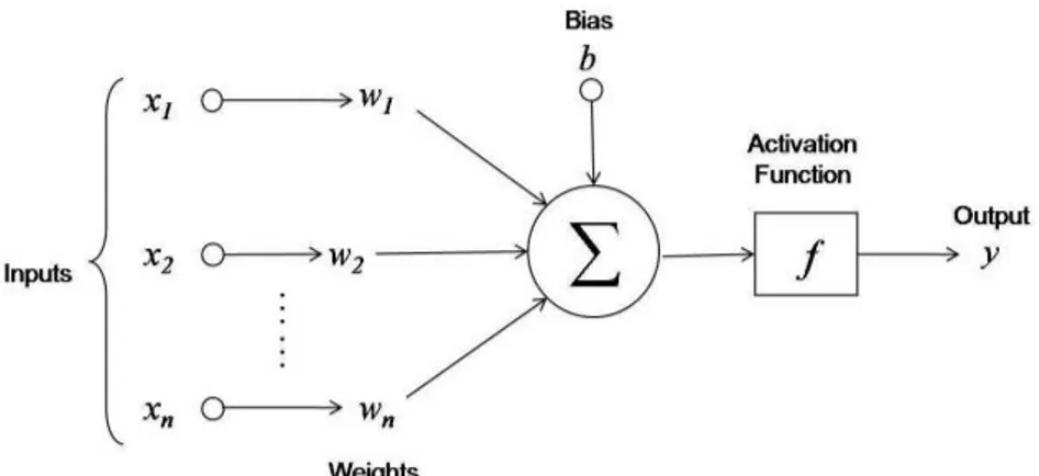
4.1 Example of artificial neuron. Input values xi are multiplies by weights wiand then summed up along with a bias vector b. The output is passed through an activation function f to produce the final output y. The actual Neuron is only the first part of the image summing pu all values along with the bias.1 36 4.2 Examples of possible activation functions.1 . . . . 37
4.3 Example of multilayer NN with fully connected layers.1. . . 38
4.4 Examples of a Convolutional layer. The depth of the features increases in the next layer1. . . . . 39
4.5 Examples of an activation map. The size of the image is reduces given that the kernel is convolved only inside the image1. . . . . 39
4.6 Examples of a pooling layer. The image is down sampled, making it smaller, but the feature depth is unchanged1. . . . 40
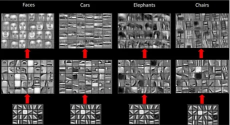
4.7 Examples of CNN features. The initial layers are similar while later layers specialise for the detected content1. . . . . 40
4.8 Figure (a) shows the inception layers as a composition of several filters[150]. Figure (b) shows skip layers allow input parameters to flow through the network making it capable of learning the identity function[73].. . . 41
4.9 Schematics representing a sequence of LSTM neurons1. . . . 42
5.1 Example bounding boxes and predicted classes using the Mask R-CNN network [66]. Each segmented object is col-ored with a different color and a label is associated to the surrounding bounding box. . . 48
5.2 Example of face recognition pipeline in OpenFace1. . . . . . 49
5.3 General detection pipeline of OpenPose1 . . . 51
5.4 Performance comparison between an integrated TX1 GPU, an Intel core i7 CPU and between a Desktop Titan X GPU and an intel Xeon processor1.. . . . 54
6.1 Mock up of the PELARS system1. . . . . 56
6.2 Image representing the Arduino Programming IDE. . . 60
6.3 Talkoo components example. . . 61
6.4 The general architecture of the PELARS Server. . . 63
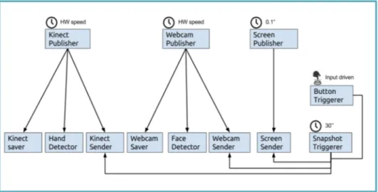
6.5 General overview of the PELARS data acquisition architecture. 64
6.7 Angle of the head motions as corresponding to the snapshots taken by the system. . . 66
6.8 PELARS desk as seen from the rgb camera. . . 67
6.9 Example of the interface for the object tracking task. . . 68
6.10 Quality of solution scores (QuaOS) of each team during the three sessions. . . 70
6.11 Neural Network structure of the model which obtained the best results . . . 74
6.12 Resulting grades of the projects output developed by the tested groups of students. . . 77
6.13 Distribution of phases among session of the 6 teams. Each session is split in the three phases, first plan, then build and finally reflect . . . 78
7.1 The Ramcip Robot.1. . . . . 84
7.2 An overview of the objectives of the RAMCIP project.1. . . . 86
7.3 Confidence level of the tracker as a function of the distance from the camera. . . 91
7.4 Time series of right foot x, y and z coordinates in the CoM reference frame during pre-fatigue task of subject one. For the whole x, y and z coordinated trajectories (black) the valid CoM estimation is highlighted in red, green and blue. . . 92
7.5 Accuracy as a function of window size and data stride. For every window size (30 samples: cyan, 60 samples: gray, 90 samples: red, 120 samples: green, 150 samples: blue) we ex-plored different data stride starting from 5 samples to window size, with increments of 15 samples. The optimal values re-sulted with a window size of 150 samples and a data stride of approximately between one tenth and a third of the window size. Median, first and third quartiles are shown, whiskers show the 1.4 interquartile range values. . . 96
7.6 Accuracy as a function of the dropout. Median, first and third quartiles are shown, whiskers show the 1.4 interquartile range values. . . 97
7.7 Accuracy as a function of the learning rate. Median, first and third quartiles are shown, whiskers show the 1.4 interquartile range values.. . . 98
7.8 Accuracy as a function of the L2 regularization. Median, first and third quartiles are shown, whiskers show the 1.4 interquartile range values. . . 98
7.9 Confusion matrices for the training set with F1 Score 0.95 (A) and for the test set with F1 Score 0.76 (B). The classification outputs are non fatigued (NF) and fatigued (F).. . . 99
7.10 ROC curves for the test set for the three approaches SVM, NN and DT. The proposed approach exhibits a greater area under the curve, compared to the other classifiers. . . 100
7.11 Classification results, fatigued (F) and non fatigued (NF), for three subjects: 1 (top), 5 (center), 15 (bottom), outputted by the trained NN. The dashed box represents the fatiguing portion of the trial; left represents the pre-fatigue phase classification (blue), right represents the post-fatigue classification (red). The blue and red vertical lines represent respectively the end of the two phases. . . 100
7.12 Representation of the correctness of the recognition as a func-tion of the distance from the camera. Note that the sampling of the points along time is affected by the windowing and confidence level of the tracking. . . 101
8.1 We use VALUE to automatically find the 3D locations of all traffic lights in Manhattan, such that they can be used for autonomous driving. Zero images were manually labeled to make this semantic map. . . 104
8.2 The 3D representation of a cluster of views with 4 contents shown as red dots. Each content is connected with the voters using a green line. The green view and the green content correspond to the one shown in the figure 8.3. . . 107
8.3 Image of the highlighted view and content of figure 8.2 show-ing the content projected over the detected position. The re-projection difference is 0.5 pixels. A detected content is a content which has been detected by the ML system, while a reconstructed content is a content which passed the voting scheme and has an associated 3D position. . . 108
8.4 The overview of the system. The final output consists of a list of 3D detections. These can be passed back into the input of the system to obtain better results. . . 109
8.5 An example of a cluster in the map consisting of several traver-sals in differing conditions. Top: Close-up of the dataset clus-tering. Bottom row: example frames that are from different traversals belonging to the highlighted cluster and associated traffic lights. . . 109
8.6 Performance of the system as a function of number of passes through a location. As the amount of data increases both recall and 3D localisation accuracy (as measured by negative reprojection error) increase. . . 114
8.7 Failure modes of the presented method. When not enough data from a particular location are provided both (a) false negative detections due to the undetected objects or (b) tem-porarily consistent wrong detections can manifest. The largest challenge is (c) consistent and repeated detections of a objects that look similar to a traffic light over a period of time. . . . 115
8.8 Number of detected contents in respect of a precision parame-ter. The precision value is multiplied by the distance threshold when voting for a content. . . 116
1.1 Mapping of RQs onto Contributions . . . 5
3.1 Qualitative evaluation for the keypoint extraction. . . 26
3.2 Qualitative evaluation for the keypoint descriptors. . . 26
3.3 Qualitative evaluation for the clustering algorithms. . . 26
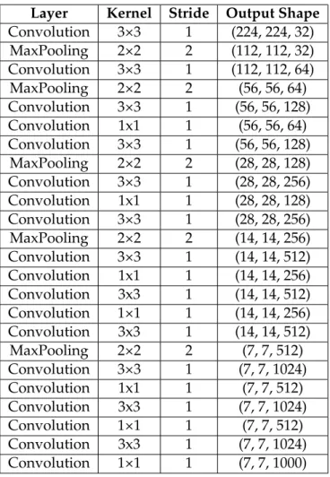
5.1 YOLO Layers. . . 46
5.2 YOLO9000 Layers. . . 46
6.1 Table of the 18 session scores organized by team. The five scores expressed in a 5 level Likert-type are reported. . . 71
6.2 Machine Learning Tasks performed over Data . . . 72
6.3 Results for the 120s window, 0.242 overall . . . 76
6.4 Results for the 240s window, 0.129 overall . . . 76
6.5 Results for the 360s window, 0.193 overall . . . 76
6.6 Best network results for the different network configurations 76 6.7 Best error scores after removing isolated features . . . 76
6.8 Effect of phases in the inclusion of the classifier. P=plan, W=work, R=reflect. Values are accuracy percentages. . . 78
7.1 Age, sex and Mini Mental State Examination Weighted Sum score, and the self-assessed level of Tiredness (1-10) for every participant at the end of the trial. . . 88
7.2 Durations of the three phases for all the subjects. . . 89
7.3 Markers provided by the skeleton tracker and the relative terminology used in this work. . . 90
7.4 Dataset composition . . . 93
7.5 Optimal hyper-parameters for the NN.. . . 96
8.1 Result of the evaluation among the algorithms. The first two columns report the average and maximum triangulated error respectively, the third is the re-projection error in pixels and the fourth the running time of the algorithm. . . 106
8.2 Per-dataset statistics of 2D detection and clustering. . . 112
8.4 Statistics of the number of passes per cluster. As the mapping fleet traverses the environment each place is visited several times. As discussed in the text more passes through the envi-ronment result into higher performance of the system.. . . . 115
AS Autonomous System AR Activity Recognition ML Machine Learning NN Neural Network DL Deep Learning
DNN Deep Neural Network
CNN Convolutional Neural Network RNN Recurrent Neural Network
R-CNN Recurrent Convolutional Neural Network DBN Deep Belief Networks
MCI Mild Cognitive Impairments
PELARS Practice-based Experiential Learning Analytics Research and
Sup-port
RAMCIP Robotic Assistant for MCI Patients at home
VALUE Large Scale Voting-based Automatic Labelling for Urban
Environ-ments
MMSE WS Mini Mental State Examination Weighted Sum Score AD Alzheimer’s Disease
ROS Robot Operating System CoM Center of Mass
MMLA Multi Modal Learning Analytics GPU Graphics Processing Unit
PAF Part Affinity Fields
ILP Integer Linear Programming
ASIC Application Specific Integrated Circuit FPGA Field Programmable Gate Array PBL Project Based Learning
RA Reference Axis RF Reference Frame
Chapter 1
Introduction
“If you look at the field of robotics today, you can say robots have been in the deepest oceans, they’ve been to Mars, you know? They’ve been all these places, but they’re just now starting to come into your living room. Your living room is the final frontier for robots.”
Cynthia Breazeal, [110]
We are starting to live exactly at the edge of time in which Robots are coming to our living rooms.
Autonomous Systems (AS) are becoming an ubiquitous reality in modern day society. In general, an AS can be defined as a robot or system that performs behaviors or tasks with a high degree of autonomy. The main goal of such systems is to improve the overall human quality of life in all possible aspects; from self driving vehicles to assistive robots. Usually robotic systems are triggered by human actions, acting on the inputs of a user. ASs instead shift this paradigm, making robots capable of anticipating human needs and actions. This implies that ASs have to be able to take decisions based on the performed activity, the general state of the person interacting with it and the surrounding environment. To do this, ASs need to have some kind of intelligence which has been studied deeply in the field of Machine Learning (ML).
ML, according to Arthur Samuel, gives "computers the ability to learn without being explicitly programmed." The term was coined by him in 1959 while at IBM. Despite being already studied for several decades, ML had only lately a major success with the rediscovery of Neural Networks (NN). Warren McCulloch and Walter Pitts (1943) created a computational model for NNs based on mathematics and algorithms called threshold logic. Since then, NNs had some minor success at character recognition in 1990 when they were used to recognise automatically recipients of post correspondence and digits on cheques. After that, NNs were not investigated much given that the high computational load could not be processed in a reasonable amount of
time on present calculators. This changed recently with the advances in GPU hardware and software and at the same time with the research advances in Deep Learning (DL) using Deep Neural Networks (DNN).
DL was introduced to the ML community by Rina Dechter in 1986 and got a major success in 2006 with a publication by Hinton et al. [69]. Since then DNN have been used to investigate several branches of computer science, creating many new fields of research and making autonomous systems a viable possibility.
Recent GPU’s have started to target ML computation, DNNs more pre-cisely, implementing dedicated hardware to be able to overcome the compu-tational problem which was afflicting them. Given that quickly GPUs were able to cope with the power demand of simple NNs, more complex networks have been created, which were able to solve complex challenges, as image recognition and detection, to a certain degree of precision. Almost human performance has been reached in the last years thanks to the discovery of Convolutional Neural Networks (CNN), which gave autonomous systems new capabilities, making the interaction between humans and machines almost natural.
Thanks to these advancements, we are starting to have the first proto-types of fully autonomous vehicles and robots, which brings up a series of challenges in the interaction between human and machine.
1.1 Research aims and questions
The aim of this thesis is to investigate the ability of ASs to detect an activity (Research Aim 1 (RA1), evaluate the state of the person interacting with the
AS (Research Aim 2 (RA2) and perceive their environment (Research Aim 3 (RA3) through modern ML techniques.
Source data is usually noisy, given that it comes from unconstrained real world scenarios. We would like to avoid the filtering of it given that usually the noise input model is unknown. ML has proven very effective at extracting strong features from input streams, making the task simpler.
This leads to the following research questions:
Research Question 1 (RQ1): Is it possible for autonomous systems to
extract high level information from a system represented by an ensemble of noisy sources of data?
feature based
2D/3D 2D/3D 3D
OBJECTS FACES BODY POSE
openface
CLNF HOGHAAR openposeRF template matching
DL | CA DETECTION CNN TASK VALUE DL | CA CLASSIFICATION TASK
PELARS SVM RAMCIPTASK SVM
DL = Deep Learning CA = Classical Approach
FIGURE1.1: General overview of the Detection and Classi-fication split analysed in this work. Each computer vision activity performed by an AS can be split in Classification and Detection. In each subfigure we present on the left side of each bar the available ML solutions and the task involved in the assessment while on the right side we present the
Each of the described tasks can be split in Detection and Classification, see figure1.1. Detection deals with the extraction of particular information from a larger stream of information while Classification deals with recog-nizing, differentiating and understanding ideas and objects. In this work Detection is used to extract semantic content from an observed scene, which can be then processed and utilised by a Classification system in order to make decisions and take actions. This leads us to the question:
Research Question 2 (RQ2): What kind of ML technique is able to solve
the Detection/Classification problem in the different explained scenarios?
Given that this work focuses on the interaction between humans and machines, we will analyse three different categories of detection: Objects, Faces and Body poses. For each of them we want to answer the following questions:
Research Question 3 (RQ3): Is it possible for autonomous systems to
detect with sufficient precision objects?
Research Question 4 (RQ4): Is it possible for autonomous systems to
detect, with sufficient precision faces?
Research Question 5 (RQ5): Is it possible for autonomous systems to
detect, with sufficient precision body poses?
It is important to notice also that all the depicted interactions between AS and humans are happening in 3D space. This poses a series of problems and questions regarding the possibility of inferring precisely a 3D position given 2D information. Nowadays 3D sensors are available, which produce depth images of space, but are more complex to interact with and have a series of limitations, which are not present in common 2D cameras. This brings us to the question:
Research Question Constributions Focus RQ1 C1, C3 Scene Understanding RQ2 C1, C2, C3 Machine Learning RQ3 C1, C3 Object Detection RQ4 C1 Face detection RQ5 C2 Pose estimation RQ6 C3, C4 Triangulation techniques
TABLE1.1: Mapping of RQs onto Contributions
Research Question 6 (RQ6): Is it possible to reconstruct, accurately
enough for an ASs, 3D information given a series of 2D measurements, or is a 3D sensors necessary for the interaction between AS and Humans?
1.2 Contributions
To answer the aforementioned research questions we developed three dif-ferent systems. Each of these system will answer partially the proposed research questions as depicted in Table1.1.
C1: The first system has been developed to create an autonomous system
capable of recognizing activities. This has been done by recognizing the actions of students during different hands on learning activities.
C2: The second system consists of an autonomous robot interacting with
elderly patients. In this context, we researched the possibility of ex-tracting non invasive measures of the state of the patient, using a 3D sensor. This was done to adapt the behavior of the robot to suit best the needs of the patient.
C3: The third system has been developed to test the ability of an
au-tonomous system to augment a urban environment. In this scenario we developed specifically a system capable of detecting and 3D localising traffic lights for autonomous driving.
C4: Additionally, to test the possibility of using 2D data to interact with
a 3D environment, we evaluated different triangulation techniques which are present in all three aforementioned systems
1.3 Involved Projects
Several projects have contributed to the research developed in this work. This section briefly introduces them.
• Practice-based Experiential Learning Analytics Research
and Support (PELARS) is a European project that studies how people
learn about science, technology and mathematics when using their hands as well as their heads. A big part of the project is making more explicit the implicit practices of science teachers: “Lab demos” and hands-on experiments have been a big part of science teaching for as long as anyone can remember, but how to model and analyse these practice, while empowering teachers, is far less understood. So, the PELARS project aims at finding ways of generating “analytics” (data about the learning process and analysis of this data), which helps learners and teachers by providing feedback from hands-on, project-based and experiential learning situations. This project will be discussed in detail in Chapter6.
• Robotic Assistant for MCI Patients at home (RAMCIP) is a European Project which aims to research and develop real robotic solutions for assistive robotics for the elderly and those suffering from Mild Cogni-tive Impairments (MCI) and dementia. This is a key step to developing a wide range of assistive technologies. We will adopt existing technolo-gies from the robotics community, fuse those with user-centred design activities and practical validation, trying to create a step-change in robotics for assisted living. This project will be discussed in detail in Chapter7.
• Large Scale Voting-based Automatic Labelling for Urban
Environ-ments (VALUE). We developed a system capable of recognizing 3D
contents in a urban environment in order to add them to a semantic map that can be used by autonomous agents to navigate it. Contents are firstly detected in 2D iamges and then views of the same content are grouped together in order to produce its 3D location in space. This project was developed jointly with Blue Vision Labs (BVL), London, UK. This project will be discussed in detail in Chapter8.
1.4 Thesis Structure
This thesis is organised as follows:In Chapter2we will present the state of the art in ASs and in classical detection systems. Chapter4and Chapter5will analyse in depth the avail-able ML solutions to the presented problems. In Chapter6we present the PELARS system along with its results, which will demonstrate the ability of an AS to do Activity Recognition (AR). After this, we will show in Chapter
7an example of non invasive extraction of human state using a 3D sensor. In Chapter8we discuss the construction and evaluation of a system capable of augmenting 3D maps. Finally in Chapter9we will discuss the achieved results and present possible future work.
Chapter 2
State of the Art
2.1 History
The idea of AS dates back several centuries, starting with early Greek myths of Hephaestus and Pygmalion who include concepts of animated statues or sculptures [31]. The first automatic devices were called "automata", which is defined as a self-operating machine or control mechanism designed to automatically follow a predetermined sequence of operations, or respond to predetermined instructions.
There are other examples in ancient China, for example in the Lie Zi text, written in the 3rd century BC. It contains a description of a much earlier encounter between King Mu of Zhou (1023-957 BC) and a mechanical engineer known as Yan Shi, an ’artificer’.
Later on, around the 8th century, we find the first wind powered au-tomata, which were defined as "statues that turned with the wind over the domes of the four gates and the palace complex of the Round City of Bagh-dad". We still can’t speak of autonomous systems given the complete lack of decision making and human interaction.
First simple ASs can be found in 1206 when Al-Jazari described complex programmable humanoid automata, which he designed and constructed in the Book of Knowledge of Ingenious Mechanical Devices. One example of an early AS was a boat with four automatic musicians that floated on a lake to entertain guests at royal drinking parties. The mechanism had a programmable drum machine with pegs (cams) that bump into little levers that operate the percussion. It was possible to play different rhythms and drum patterns if the pegs were moved around.
During the Reneissance the studies of automata witnessed a considerable revival. Numerous clockworks were built in the 16th century, mainly by the goldsmiths of central Europe. Leonardo da Vinci started sketching and building hundreds of automatic machines, making the interest in such devices grow in the next centuries.
All these examples can not be regarded as ASs given that they were still mainly mimicking human and were mainly considered objects of art than of engineering. In more recent history, a new field of science was born, Cybernetics, which filled the gap between automatas and ASs . Norbert Wiener defined cybernetics in 1948 as "the scientific study of control and communication in the animal and the machine" [167]. He was a mathematics professor at MIT working to develop automated rangefinders for anti-aircraft guns with “intelligent” behavior [68].
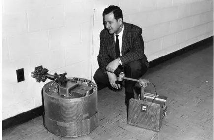
This theory motivated the first generation of ASs research in which sim-ple sensors and effectors were combined with analog control electronics to create systems that could demonstrate a variety of interesting reactive behaviors. In 1964 one of the first AS was built by the APL Adaptive Ma-chines Group, led by Leonard Scheer at the John Hopkins University. They built an autonomous rover system capable of navigating the APL’s hallways, identifying objects as electrical outlets in the walls, which it could use to plug itself in to recharge its battery, see Figure2.1.
FIGURE2.1: An image showing the autonomous rover built by the APL group in 19641.
1http://cyberneticzoo.com/tag/autonomous/
With the advent of digital electronic controllers and the new born interest in artificial intelligence [166,56], more complex autonomous systems were built. The new systems were used in several different fields, but mainly for military purpose initially. We have many examples in several domains as maritime, air, ground and space vehicles [156].
In modern days, ASs became widespread and a series of common sub-problems were categorized. Each AS needs to self maintain itself, sense and navigate the environment, perform tasks, learn from its history.
2.2 Self Maintenance
A fundamental requirement for complete physical autonomy is the ability of a robot to be aware of its internal state. This ability is called "proprioception". Many of the commercial robots available in the market today can find and connect autonomously to a charging station, like Sony’s Aibo (Figure2.2a) or Ugobe’s Pleo (Figure2.2b).
(A) (B)
FIGURE2.2: Example of two robots capable of connecting autonomously to a charging station. Figure (a) shows Sony’s
Aibo1and Figure (b) shows Ugobe’s Pleo2.
1http://www.sony-aibo.com/
2http://www.pleoworld.com/
In the battery charging example, the robot can tell proprioceptively that its batteries are low, and it then seeks the charger. Other examples of proprioceptive sensors are thermal, optical and haptic, as well as those measuring the Hall effect (electric) [63]. These abilities will be required more and more for robots in order to work autonomously near people and in harsh environments. Autonomous rovers used to explore extraterrestrial planets need often to work autonomously for several years, without the possibility of any physical maintenance [159].
This brought to the development of even more advanced systems capable of self repairing [52]. In this case the system is able not only to asses an incorrect self state, but also to remedy it by taking appropriate actions. It is important to notice that this kind of failures can affect both hardware and software.
2.3 Sensing and Navigating
Autonomous systems need to sense the environment in order to navigate it [93,42]. To do this they are usually equipped with a set of sensors, which allow them to perceive the space surrounding them. The most common sensors are 2D cameras and depth sensors [9]. Both are usually used to
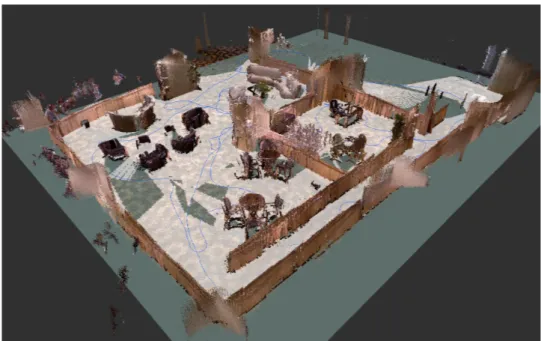
construct a 3D map of the explored space in order to avoid obstacles and to map unknown areas, Figure2.3.
FIGURE2.3: An example of 3D mapped environment from the IROS 2014 Challenge1.
1https://github.com/introlab/rtabmap/wiki/
IROS-2014-Kinect-Challenge
Examples of other sensors used to understand the environment are: electromagnetic spectrum, sound, touch, smell, temperature and altitude.
Within the depth sensors, a great variety of models is available, from commercial ones as the Kinect v1 and Kinect v2 [164] to more precise models like laser scanners. The first ones are less accurate (v1 ≥ 1.5 mm at 50 cm. About 5 cm at 5 m), but cheap, while laser scanners are much more precise (<1mm), but are more expensive. It is also important to notice that the different systems have different update frequencies. This it not relevant if static scenes are scanned, but it can cause problems when fast moving objects are scanned. While commercial sensors have frequencies between 30Hz and 60Hz, laser scanners can reach over 1KHz for single scanned line.
Many ASs are hence equipped with stereo cameras, which are also capa-ble of inferring the depth. These cameras have the advantage that they are usually cheaper, don’t need specialised software and have more software support. We will analyse in a Section8.2the advantages and disadvantages of 2D sensors against depth sensors.
2.4 Performing tasks
Once the environment has been sensed, the ASs need to take actions in order to fulfill a certain objective. To do this, the AS need to be able to take conditional decision, which are usually determined by some machine learning algorithm [120].
An example of such a system can be found i the Cataglyphis rover. This robot has demonstrated, during the final NASA Sample Return Robot Cen-tennial Challenge in 2016, fully autonomous navigation, decision-making, sample detection, retrieval, and return capabilities. The rover relied on a fusion of measurements from inertial sensors, wheel encoders, Lidar, and camera for navigation and mapping.
More common examples of self adapting systems can be found for ex-ample in robotic lawn mowers [45], which can adapt their programming by detecting the speed at which grass grows or some vacuum cleaning robots [137], which are able to sense how much dirt is being picked up and use this information to plan the amount of time spent in different areas.
Usually these systems try to maximize an objective score given by an objective function. Classically this could be done using calculus trying to minimize a cost function or maximizing an objective score. Nowadays Reinforcement Learning (RL) is used to train directly an AS by examples without having the need to define an objective function, but by just defining an objective score. This made it possible to train easily non linear function which gave promising results lately [101].
Very often ASs need to manipulate objects. To do this they need to firstly identify an object in space and then compute the objects pose. A pose is defined by 6 degrees of freedom, 3 for rotation and 3 for translation. A classically approach to solve this problem consists in the use of descriptors, which can be seen as strong invariant features of an object. Techniques which are based on this have the disadvantage of being influenced strongly by external factors as lighting conditions. Nowadays DL techniques are used to overcome the problems which come from having different environments. These techniques are able to find stronger features which are no man crafted, adapting better to real world scenarios. We will present in the next chapter the classical approaches and in Chapter4the more recent techniques.
Chapter 3
Classic Detection
“There is nothing more deceptive than an obvious fact.” Arthur Conan Doyle, [40]
3.1 3D Object Detection
This chapter will introduce the state of the art in detection algorithms not based on ML, but on classical computer vision techniques. The general pipeline for a 3D object recognition algorithm, which identifies a model in a scene, consists of the following steps:
• Preprocessing of the depth and RGB images. This step is used to filter the image from noise and unnecessary information. The two images are then merged together to create a point cloud. Segmenting and filtering objects by color can improve significantly performances and should always be done when possible.
• Extraction of keypoints from the model and the scene. Keypoints are point of interest that carry a big amount of information given their position and color.
• Creation of a descriptor for each keypoint. Given that keypoints could change from the model to the scene due to light, different scales and deformations, a descriptor is used to describe each keypoint. In general a descriptor consists of a set of attributes, which are scale invariant and flexible to deformation and noise, of the keypoint and its surrounding.
• Matching of scene and model descriptors. The general strategy consists in calculating a distance between each descriptor of the model and the scene. If the distance is lower than a certain threshold then the two descriptors are matched.
• Clustering of the found correspondences between descriptors. This step is used to avoid sparse correspondences which are of no interest.
The results are clustered since a good match between the model and the scene is found only when a big number of correspondences is found in a relative compact space.
• Examine a plausible solution and estimate a possible object pose. All the clusters are evaluated using some voting scheme and, if good enough ,a possible pose is estimated using the previously found corre-spondences.
The first three steps have to be performed on the model and on the scene, Figure3.1. It is important to notice that they are computed only the first time on the model and have to be recomputed for each new scene point cloud.
FIGURE3.1: 3D object recognition pipeline1. For each input
image, keypoints are extracted. The next step consists in the computation on features to describe the local region around keypoint. Matches between descriptors are computed based on a distance metric and positive ones are clustered. Finally a transformation from the input object to the clustered points
is estimated.
3.1.1 Models
Creating 3D models remains a quite difficult task, expecially when creating models of small objects like a cup or a fork. It is possible to create model using low cost depth cameras, but there are mainly two problems:
• Homogeneous objects have few geometric features making it hard to understand the current object position while moving around the scanner. To avoid this problem it is often enough to place some other objects around the model or to use markers. The drawback of this solution is that there is the need of some post processing to remove the additional objects.
• Most scene reconstruction algorithms are made for rooms or big scenes and tend to approximate small objects; this leads to the problem that a lot of key-geometrical structures get lost. As an example if you try to scan a rubick cube you will probably just get a uniform cube.
There are some specialized libraries for scene reconstruction like kinectfusion and the opensource version kinfu, but both suffer of the described problems. There are also specialized 3D scanners of different dimensions which give professional results, but they come at a higher price.
3.1.2 Keypoint Extraction
Keypoint extraction is done using either RGB or depth information. There are three main categories of keypoints that can be subdivided based on the cloud information which are used. A genera survey can be found in [154]. Here we will present just a few of the most commonly used keypoint detectors.
1. RGB:
• SIFT [97] (Scale-Invariant Feature Transform) is one of the most used algorithms , which works analysing the RGB values of the point cloud. To find points of interest SIFT tries to locate points which have a high color gradient with the sorrounding. This points usually belong to figure edges or relevant images on uni-form surfaces.
• SURF [10] (Speeded Up Robust Feature) is several times faster and more robust against different image transformations than SIFT. It uses an integer approximation of the determinant of Hessian blob detector. The determinant of the Hessian matrix is used as
a measure of local change around the point and keypoints are chosen where this determinant is maximal.
• FAST [162] (Features from Accelerated Segment Test) is a corner detection method. The algorithm is very efficient computationally and in general is one of the fastest keypoint detectors available. To detect keypoinys, FAST evaluates a circle of 16 pixels to classify whether a candidate point is a corner. If a set of contiguous pixels in the circle are all brighter than the intensity of the candidate pixel plus a threshold value or they are all darker than the in-tensity of candidate pixel minus a threshold, then the candidate point is classified as corner.
• ORB [131] (Oriented FAST and Rotated BRIEF) aims to provide a fast and efficient alternative to SIFT. ORB consists in a fusion of the FAST and BRIEF descriptor with several modifications to enhance performance. It uses FAST to detect keypoints and Harris to detect the best ones among them. An additional enhancement has been added to make the detector rotation invariant.
• SUSAN [143] (Smallest Univalue Segment Assimilating Nucleus) uses a circular region to detect if a candidate pixel is a keypoint.; the candidate pixel is called nucleus. Similarly to FAST is uses a comparison function to evaluate the pixels in the area and determine if the nucleus is a keypoint or not. The function is based mainly on the brightness difference threshold of the pixels in the area.
• Harris [39] is capable of identifying similar regions in images taken from different viewpoints that are related by a simple ge-ometric transformation: scaling, rotation and shearing. To do this, the algorithm follows a sequence of steps which consists in: Identify initial region points using scale-invariant Harris-Laplace Detector, normalize each region to be affine invariant using affine shape adaptation, select proper integration scale, differentiation scale and spatially localize interest points, update the affine re-gion using these scales and spatial localisations and finally iterate the previous steps if the stopping criterion is not met.
2. DEPTH:
• NARF [147] (Normal Aligned Radial Feature) works by analysing the depth values of the point cloud. To find points of interest
NARF tries to find points for which the depth value changes rapidly in their sorrounding. This technique allows to find edge points which are of particular interest in 3D images.
• 3D SURF [83] is an extension of SURF which is based on the vox-elization of an input cloud. Each produced bin is then described using a modified version of SURF.
3. RGB and/or Depth: Sampling has two working modes: Uniform and Random. Uniform sampling is very fast and scans the whole scene, but in principle acquires more points than necessary if the model in the scene occupies only a small fraction of it. Random sampling in contrast can be tuned on the number of desired points but could in principle get keypoints of undesired areas.
3.1.3 Keypoint Descriptors
Descriptors are needed since matching single keypoints is unfeasible given scale, light and rotation changes from the model to the scene. To avoid all these problems, not single keypoints are matched, but regions surrounding the keypoints. This includes cubic regions, spheres (Figure3.2), couples of points with their direction relatively to the keypoints and so on. In general a descriptor defines a keypoint and its surrounding.
FIGURE3.2: Spherical reference frame for a descriptor1.
1http://pointclouds.org/documentation/tutorials/how_
features_work.php
Descriptors can be local, Figure3.4, or global, Figure3.3; the first ones consider the keypoints relatively to a small surrounding region, while the second ones consider the entire scene . There are three main descriptors which represent the main descriptor categories: FPFH [134] , SIFT [97] and Shot [135]; all of them can be found in different flavors with small variations. In general we have signature based methods and histogram based methods. The first ones describe the 3D surface neighborhood of a given point by defining
an invariant local Reference Frame (RF). This frame encodes, according to the local coordinates, one or more geometric measurements computed indi-vidually on each point of a subset of the support. Histogram-based methods describe the support by accumulating local geometrical or topological mea-surements (e.g. point counts, mesh triangle areas) into histograms according to a specific quantized domain (e.g. point coordinates, curvatures . . . ). This domain requires the definition of either a Reference Axis (RA) or a local RF. In broad terms, signatures are potentially highly descriptive thanks to the use of spatially well localized information, whereas histograms traoff de-scriptive power for robustness by compressing geometric structure into bins. FPFH is a histogram based descriptor, SIFT is a signature based descriptor and Shot is both a signature and histogram based descriptor.
1. FPFH (Fast Point Feature Histogram) is a faster to calculate version of PFH (Point Feature Histogram). The goal of the PFH formulation is to encode a point’s k-neighborhood geometrical properties by generaliz-ing the mean curvature around the point usgeneraliz-ing a multi-dimensional histogram of values. The figure below presents an influence region diagram of the PFH computation for a query point, marked with red and placed in the middle of a circle (sphere in 3D) with radius r, and all its k neighbors (points with distances smaller than the radius r) are fully interconnected in a mesh. The final PFH descriptor is com-puted as a histogram of relationships between all pairs of points in the neighborhood, and thus has a computational complexity of O(k2).
FIGURE3.3: Histogram based descriptor1. 1https:
2. SIFT (Scale Invariant Feature Transform) descriptor, a signature based descriptor, uses the gradient information of a region around the key-point to create a descriptor. Color gradient is used to encode the changes around the keypoint. To be more precise SIFT relies on a set of local histograms, that are computed on specific subsets of pixels defined by a regular grid superimposed on the patch. Later on also RGB has been introduced as an additional feature in some versions of the SIFT descriptor
FIGURE3.4: Signature based descriptor1. 1http:
//pointclouds.org/documentation/tutorials/pfh_estimation.php
3. SHOT (Signature of Histograms of OrienTations) descriptor combines the advantages from both signature based methods and histogram based methods. It encodes histograms of basic first-order differential entities (i.e. the normals of the points within the support), which are more representative of the local structure of the surface compared to plain 3D coordinates. The use of histograms brings in the filtering effect required to achieve robustness to noise. Having defined an unique and robust 3D local RF, it is possible to enhance the discriminative power of the descriptor by introducing geometric information concerning the location of the points within the support, thereby mimicking a signature. This is done by first computing a set of local histograms over the 3D volumes defined by a 3D grid superimposed on the support and then grouping together all local histograms to form the actual descriptor.
4. BRIEF [22] (Binary Robust Independent Elementary Features) was developed to lower the memory usage of keypoint detectors and de-scriptors, in order to be used in memory constraint systems. BRIEF uses smoothened image patches and selects a set of location pairs in an unique way. Then some pixel intensity comparisons are done on these location pairs. For each location a quick comparison function is evaluated to produce a binary string which can be used as a descriptor.
5. HOG [38] (Histogram of oriented Gradients) will be described more in detail in connection with its use for face detection in3.2
3.1.4 Matching Descriptors
Given two sets of descriptor vectors coming from two acquired scans, there are two methods to find corresponding descriptors. It is possible to match descriptors or keypoints, depending if the point clouds are organized; a point cloud is "organized" if there is a viewpoint in space where the point cloud can be described like an image (X, Y coordinates) and a last parameter: depth. It is possible to match points or descriptors, even if, as stated previously, point matching is not a good solution. The following three methods are available:
1. Brute force.
2. Indexing using KD-trees, K-Means trees etc.
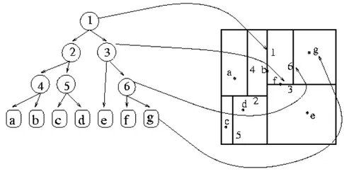
3. Using organized data to search for a correspondence in a small region. To find the best matches between model and scene descriptors, FLANN (Fast Library for Approximate Nearest Neighbors) [103] is one the most popular choices. FLANN is a library for fast approximate nearest neighbor searches in high dimensional spaces. It is a specific implementation of a KD-tree, see Figure3.5, or k-dimensional tree, which is a data structure used for organizing points in a space with k dimensions. Model descriptors or scene descriptors are inserted into a KD-tree; for each descriptor of the other set, the nearest neighbor in the KD-tree is found. Once two desriptors are matched, a correspondence is created and stored. In general all algorithms used for minimum distance search can be used to match descriptors, depending on the search space dimensions.
Naturally, not all estimated correspondences are correct. Since wrong correspondences can negatively affect the estimation of the final transforma-tion, they need to be rejected. This could be done using RANSAC (RANdom SAmple Consensus) or by trimming down the amount of correspondences using only a certain percent. RANSAC is an iterative method to estimate pa-rameters of a mathematical model from a set of observed data that contains outliers. It is a non-deterministic algorithm in the sense that it produces a reasonable result only with a certain probability, with this probability in-creasing as more iterations are allowed. RANSAC works very well with well structured objects which have a "geometrical" shape. This method tries to extract keypoints that lie on the geometrical structure specified; for example
FIGURE3.5: Example of a KD-tree1.
1http://groups.csail.mit.edu/graphics/classes/6.838/S98/
meetings/m13/kd.html
if a plane is specified then RANSAC will try to find keypoints which lie on a plane.
There is also the possibility of using PPF (Point Pair Features)[43], four-dimensional descriptors of the relative position and normals of pairs of oriented points on the surface of an object ; this algorithm covers the whole recognition pipeline, implementing a custom version of each step. Compared to traditional approaches based on point descriptors, which depend on local information around points, this algorithm creates a global model description based on oriented point pair features and matches the model locally using a fast voting scheme. The global model description consists of all model point pair features and represents a mapping from the point pair feature space to the model, where similar features on the model are grouped together. Such a representation allows to use much sparser object and scene point clouds, resulting in very fast performance. Recognition is done locally using an efficient voting scheme, similar to the Generalized Hough Transform, to optimize the model pose, which is parametric in terms of points on the model and rotation around the surface normal on a reduced two-dimensional search space. Descriptors are matched using a hash table that allows an efficient lookup during the matching phase. This method could be used in principle to match any kind of descriptor.
3.1.5 Clustering Correspondences
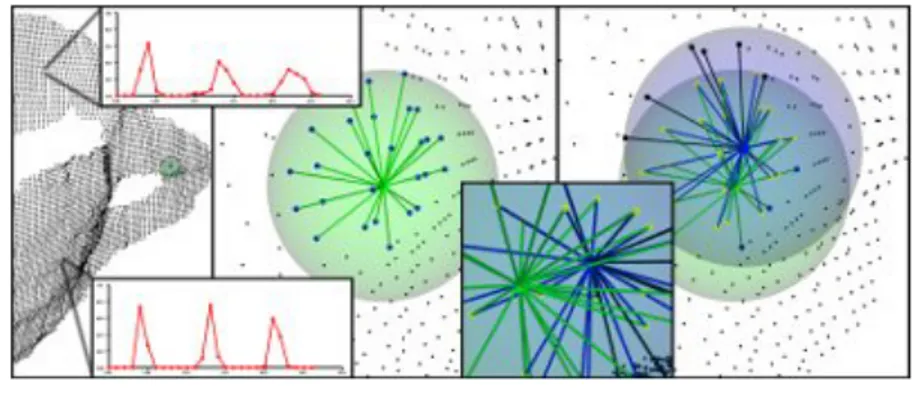
This step is used to avoid sparse correspondences which are of no interest. The found correspondences are clustered since a good match between the model and the scene is found, see Figure3.6, only when a big number of correspondences is found in a relative compact space. A possible method
is called General Hough Trasform (GHT) [6]; this method is based on the Hough Transform (HT), which is a popular computer vision technique originally introduced to detect lines in 2D images. Successive modifications allowed the HT to detect analytic shapes such as circles and ellipses. Overall, the key idea is to perform a voting of the image features (such as edges and corners) in the parameter space of the shape to be detected. Votes are accumulated in an accumulator whose dimensionality equals the number of unknown parameters of the considered shape class. For this reason, although general in theory, this technique can not be applied in practice to shapes characterized by too many parameters, since this would cause a sparse, high-dimensional accumulator leading to poor performance and high memory requirements. By means of a matching threshold, peaks in the accumulator highlight the presence of a particular shape in the image. The GHT extends the HT to detect objects with arbitrary shapes, with each feature voting for a specific position, orientation and scale factor of the shape being sought. To reduce the complexity, the gradient direction is usually computed at each feature position to quickly index the accumulator.
GHT has though well known limitations to deal with 3D shapes and 6-degree-of-freedom poses (in particular, curse of dimensionality and sparse-ness of the voting space). To avoid this problem a more general RANSAC approach is often used.
FIGURE3.6: An example of "Good" correspondences1.
1http://pointclouds.org/documentation/tutorials/
correspondence_grouping.php
Another possible algorithm is Geometric Consistency (GC) [24]. This algorithm is based on a mathematical condition that checks the consistency of pairs of correspondences in the 3D space. It can be used in combination
with a local surface descriptor for surface representation. A local surface descriptor is characterized by its centroid, its local surface type and a 2D histogram. The 2D histogram shows the frequency of occurrence of shape index values vs. the angles between the normal of reference feature point and that of its neighbors. Instead of calculating local surface descriptors for all the 3D surface points, they are calculated only for feature points that are in areas with large shape variation. In order to speed up the retrieval of surface descriptors and to deal with a large set of objects, the local surface patches of models are indexed into a hash table. Given a set of test local surface patches, votes are cast for models containing similar surface descriptors. Local surface patches candidate models are hypothesized based on potential corresponding.
The first algorithm performs better in most situations, but is slower while the second one is faster, but generates a lot of false positives that have to be filtered. GHT has also the advantage that it can be fine tuned, while GC allows for almost no tuning.
3.1.6 Estimate Object Pose
After clustering the accepted correspondences and voting for each result, a set of possible solutions is extracted along with a possible pose using the GHT. The pose can then be refined using a registration algorithm. The registration procedure consists in the process of aligning two point clouds to obtain the minimum distance between them. A famous iterative example of such an algorithm is Iterative Closest Point (ICP) [173]; in this algorithm, one point cloud, the reference or target, is kept fixed, while the other one is moved to best match the reference. This algorithm iteratively revises the transformation (combination of translation and rotation) needed to minimize the distance from the source to the reference point cloud. The basic steps are the following:
1. For each point in the source cloud find the nearest point in the reference cloud.
2. Estimate the combination of rotation and translation using a mean squared error cost function that will best align each source point to its match found in the previous step.
4. Iterate over the previous steps until some convergence criterion is met, usually a fixed number of iterations or a distance error between source and reference point cloud.
The main disadvantage of such an algorithm relies in its high resource demand due to the ICP complexity; in fact to obtain real time results quality parameters have to be lowered. The main advantage of this algorithm is that it achieves very good alignment results, refining the initially estimated pose. If used to make only small alignments, fast results can be achieved with minimum effort.
A faster version of ICP exists and is called projective-ICP [50], but it needs a good initialization. There exists also a GPU implementation of such algorithm which improves drastically the speed and is used in applications as KinectFusion [109]/
3.1.7 Qualitative Analysis
The following tables3.1,3.2,3.3show a qualitative analysis of the different proposed methods in terms of the different pipeline steps required in an object recognition pipeline.
Quantity Quality Used info
NARF Low High Depth
SIFT High Medium Color
Sampling Variable Randomic
-PPFE Low High Depth
TABLE3.1: Qualitative evaluation for the keypoint extrac-tion.
Time Quality Type SHOT Fast High Hist. & Sig. FPFH Slow Medium Signature
SIFT Slow High Histogram
PPFE Fast High Signature
PFH Very Slow Medium Signature TABLE3.2: Qualitative evaluation for the keypoint
descrip-tors.
Time Quality Flexibility
Hough Fast High High
Geometric Fast Low Low
TABLE 3.3: Qualitative evaluation for the clustering algo-rithms.
3.1.8 Measurements
It is important to measure the quality of the recognized object in the scene; to do this three main quantitative measures have to be considered, which have to be added to the qualitative measures displayed in Figure3.1.7:
• If the object is recognized.
• What is the error in the pose estimation. • Robustness against cluttering and noise.
The first parameter can be evaluated on standard datasets, calculating false positives and false negatives. It is quite complex to find false positives and false negatives without having a human analyzing the scene and comparing it to the detected object. One possible solution is to align the recognized object with the scene using a registration algorithm as ICP and then calculate the fitness of the alignment. The main problem in this case is to find a good threshold for the fitness value, which can discriminate false positives and false negatives.
The second parameter is evaluated calculating the distance and rotation error between the estimated object and the real object [75]. A lot of different measures ( ) have been implemented to compute the difference of two rotations expressed as quaternions (q1, q2) or rotation matrices (R1, R2), like:
1. Inner Product of Unit Quaternions: 3 : S3◊ S3 æ R+,
3(q1, q2) = arccos(|q1· q2|) 2. Geodesic on the Unit Sphere:
6 : SO(3) ◊ SO(3) æ R+,
6(R1, R2) = Î log(R1R2T)ÎF
where Î . . . ÎF denotes the frobenious norm,log(R) = ◊
2 sin(◊)(R ≠ RT) and1 + 2 cos(◊) = T r(R).
The third error can be estimated adding a constant uniform gaussian noise, occluding a fixed percentage of the object and then calculating the previously described errors. It is important to notice also that all this mea-sures make sense assuming that the algorithm remains real-time or almost real-time since we are evaluating ASs that interact with humans. This gives a strong constraint when trying to optimize the quality of the detector. By this we mean that relaxing this condition allow to get almost arbitrary good results.
3.1.9 Multi Object Detection
Detecting N objects in a scene increases a lot the computational requirements of the algorithm. Some stages of the pipeline remain almost the same and do not add any overhead, like the calculation of keypoints and descriptors for each model which can be done offline in a preliminary phase. The main performance issue is given in the comparison of the descriptors from the models and the scene; in the worst case we have O(k2) comparisons, which slows down a lot the detection process. A first solution could be to create in parallel N different detectors, but this depends on the number of available processing cores. Acceptable results can still be achieved having small point clouds and a good pre-filtering stage that removes all the non interesting regions [29].
3.1.10 Final Remarks
As described before there is no perfect solution to the problem of detecting an object in a 3D scene in real time. The pipeline remains very complex and needs a lot of parameter tuning to obtain good results, depending too much on the input, which has to be recognized. The algorithms need to be imple-mented efficiently on GPU to obtain good performance results, since now the computational complexity is too demanding. ML approaches simplify drastically the problem given that the parameters are learned automatically by the system and computation can be easily done on GPUs by default.
3.2 Face Detection
The most used classical face detection algorithm remains the Viola and Jones [161] one that is based on Haar features. Another well known algorithm is based on HoG. Both approaches are based on Support Vector Machines (SVM), which was one to the most used ML techniques before the rediscovery of NNs, as described previously. We will describe in the following both approaches specifying the critical aspects that made such systems perform worst than newer systems based on CNNs.
3.2.1 Haar Detector
A Haar detector is a machine learning based approach where a cascade function is trained from a lot of positive and negative images. It is then used to detect objects in other images. This kind of detector is based on Haar features that are usually computed over rectangular pixel areas.
A Haar-like feature considers adjacent rectangular regions at a specific location in a detection window. The value of a feature corresponds to the difference between sums of pixel intensities in different regions. A 2-rectangle feature, Figure3.7(a), consists in the sum of the pixels in the white rectangle area minus the sum of the pixels in the black rectangle area. A three-rectangle feature computes the sum within two outside rectangles subtracted from the sum in a center rectangle, Figure 3.7 (b). Finally a four-rectangle feature computes the difference between diagonal pairs of rectangles, Figure3.7(c).
FIGURE3.7: Example of Haar features. (a) represents a 2-rectangle feature, (b) represents a 3-2-rectangle feature and (c)
represents a 4-rectangle feature1.
1http://docs.opencv.org/trunk/d7/d8b/tutorial_py_face_
detection.html
This kind of features can be used, for example, to identify faces noticing that the region around the eyes is darker than the region of the cheeks. Therefore a common Haar feature for face detection is a set of two adjacent rectangles that lie above the eye and the cheek region, Figure 3.8. The position of these rectangles is defined relative to a detection window that acts like a bounding box to the target object .
FIGURE3.8: Example of Haar features in face recognition1.
1http://docs.opencv.org/trunk/d7/d8b/tutorial_py_face_