Polarization multistability and instability in a nonlinear dispersive ring cavity

446 J. Opt. Soc. Am. B/Vol. 11, No. 3/March 1994

Polarization multistability and instability

in a nonlinear dispersive ring cavity

M. Haelterman,* S. Trillo, and S. Wabnitz

Fondazione Ugo Bordoni, Via Baldassarre Castiglione 59, 00142 Rome, Italy

Received March 1, 1993; revised manuscript received August 18, 1993

We study the role of polarization in modulational instabilities in a synchronously pumped ring resonator that is filled with an isotropic nonlinear dispersive medium. To describe nonlinear propagation of the polarized field through the ring, we introduce two coupled driven and damped nonlinear Schrodinger equations. These equations, which result from averaging propagation and boundary conditions over each circulation through the ring, permit a simple stability analysis. This analysis predicts polarization multistability in the steady state as well as the emergence of stable pulse trains whose polarization state is either parallel or orthogonal to a linearly polarized synchronous pump beam. The analytical predictions are confirmed and extended by numerical simulations of polarized wave propagation in the cavity.

1. INTRODUCTION

Passive nonlinear cavities are well known and widespread devices in optics and are convenient experimental test beds for the investigation of fundamental nonlin-ear dynamical processes such as multistability,' self-oscillations,2 modulational instabilities,3 4 and chaos.5 6 Applications of nonlinear cavities range from optical data storage"7 to ultrafast switching,8 pulse reshaping,9 and ultrashort pulse train generation.3'4"s'2 In particular, the potential for ultrashort pulse generation of single-mode fiber-based cavities has been demonstrated by different schemes, among which we may quote the additive-pulse mode-locked (APM) laser"l and the mod-ulational instability (MI) laser.3 4"2 In APM lasers the fiber cavity is added to the main laser cavity to achieve mode locking, whereas in MI lasers the fiber ring forms the main cavity.

In a MI laser the pulse train builds up from noise be-cause the nonlinear parametric (degenerate four-photon) interaction with the pump beam selects and amplifies a weak modulation. In the cavity a pulse train results from a balance between the output coupling losses and the parametric gain, owing to the coherent and periodic amplification at the expense of the synchronous pump. Because of the coherent interference at the beam split-ter (or fiber coupler) of the cw or quasi-cw input pump with the circulating field, the cavity detuning directly en-ters into the phase-matching condition of the parametric interaction.3'4 In fact, it has been predicted recently that MI lasers, similar to APM lasers, may also operate in the normal dispersion regime (where MI in a cavityless fiber is forbidden), thanks to the detuning-induced phase matching.4 This result was analytically predicted by the linear stability analysis of a single driven-damped nonlin-ear Schrodinger (NLS) equation that describes the pulse-formation process in the cavity once the input-output boundary conditions and the fiber propagation are

aver-aged over each circulation. 3 5

However, in the scalar treatment of Refs. 3 and 4 the

polarization state of the field was not taken into account. As is well known, nonlinear polarization rotation may play an important role in the cavityless propagation and instabilities of the field. In particular, so far as MI is concerned, including the extra degree of freedom that is provided by polarization may drastically change the stability conditions of the propagating waves. For ex-ample, in an isotropic (that is, nonbirefringent) nonlinear medium a linearly polarized wave is modulationally un-stable in the anomalous dispersion regime with respect to the growth of perturbations with the same polariza-tion, whereas in the normal dispersion regime MI may occur only through the cross-phase-modulation coupling between two guided modes with different frequencies3 or orthogonal polarization.4-16 In the last case, MI leads to the growth of modulations that are orthogonally polarized with respect to the pump. This polarized MI may be seen as a breaking of the symmetry between the equally intense two circular polarization components of the field.1 4 Whenever linear birefringence is included, the MI of a continuous linearly polarized wave that is aligned with one of the fiber axes may lead both in the anomalous and in the normal dispersion regime to the growth of orthogonally polarized sidebands.'6

These considerations motivate our interest in inves-tigating the role of polarization in the process of pulse train formation from MI in fiber rings. In this paper we study polarization effects in the MI laser and consider for simplicity a linearly polarized pump field and a zero linear birefringence of the fiber. We are concerned mainly with the fiber-based MI laser (see Fig. 1); nevertheless our treatment also applies to the general case of field propa-gation in a cavity that contains a dispersive medium char-acterized by the isotropic nonlinear susceptibility tensor

Xijkl. In fact, a nonlinear Fabry-Perot resonator with a

completely reflecting mirror is a bulk equivalent of the fiber ring cavity.

As we shall see, even in the simplest case of an isotropic medium, including polarization effects leads to rich and complex dynamics that could not be anticipated from 0740-3224/94/030446-11$06.00 ©1994 Optical Society of America

x

V

at

tR

PBSz -Y

Fig. 1. Schematic of the nonlinear dispersive fiber ring cavity; 0 and p are the transmission and reflection coefficients for the amplitudes, respectively. The polarization beam splitter (PBS) is used to discriminate the two x- and y-polarization components in the output, and the pump is linearly polarized along the x axis.

the scalar approximation. A MI laser is just one ex-ample of the feedback structures for which polarization instabilities may occur. Therefore the results of this paper may be of interest for extending the study of the role of polarization to other passive nonlinear fiber-based resonators such as APM lasers.

2. COUPLED EQUATIONS AND LINEAR STABILITY ANALYSIS

The device is schematically depicted in Fig. 1. It consists of a ring cavity, in which a single-mode, dual-polarizations fiber is the nonlinear dispersive medium. The cavity is synchronously pumped by a periodic train of linearly polarized pulses in such a way that after each round trip the pulse in the cavity overlaps on the beam splitter (transmission 0, reflection p) with the subsequent input pump pulse. The polarization beam splitter is used to separate the polarization components of the output field. In the nth passage through the nonlinear material that fills the cavity, the envelope amplitudes of the two counterrotating circularly polarized modes, say En =

En(Zn, T), obey the coupled-mode equations14₁5

aE+n G1 2E+n

ZJZn 2 aT2

+ ( 1-B

1E+n12

+ + B _n12E+n = (la)

+

2

-I

1

±=,(a

aE_n -li a2E_

aZn 2 aT2

+ ( 1-B E

2'' 2 /

n12 + 1

+

B

E

+nJ2E

o

_(lb) where T is the time in the reference frame that trav-els with the common group velocity of the orthogonal cavity pulses, /3" is the group-velocity dispersion, y = 2co0n2/cAeff, and n2 and Aeff are the nonlinear refrac-tive index and the effecrefrac-tive core area, respecrefrac-tively. Fol-lowing the notation of Refs. 14-17, the parameter B =

(3) 3

XA1221(Cw; c, c, -&/X1A,(co; c, w, -) characterizes the isotropic nonlinear material that fills the cavity. For simplicity, in Eqs. (1) we neglect the linear birefringence of the fiber.

When we assume a polarization-insensitive beam split-ter (or coupler) and a linearly polarized input field, the cavity boundary conditions read as

E 4+'(Z, = 0, T) = Ei(T) + p exp(-io)E±'(Zn

=

L, T),

(2) where L is the cavity length, 0 and p are the amplitude transmission and reflection coupling coefficients (that is,

02 + p2 = 1), 0 is the linear phase detuning of the cavity,

and E1(T) are the (equal) circular components of the

quasi-cw linearly polarized pump pulse.

The polarization dynamics of the nonlinear fiber ring is ruled by the map of Eqs. (1) and (2). The study of the nonlinear fiber resonator by means of Eqs. (1) and (2) calls for a numerical solution to the problem. An important physical insight in the vector pulse formation process may be provided by the linear stability analysis of averaged equations that give good approximation to Eqs. (1) and (2) under appropriate restrictive conditions. In fact, we have already shown that in the scalar case Eqs. (1) and (2) may be averaged to a single partial derivative equation (PDE)34 under the main hypotheses of (a) high-finesse cavity, that is, we may set the cavity reflectivity p = (1 - 02)S12 _ 1 - 012/2, where << 1; (b) small cavity detuning, that is, we set 1/vr = e (for simplicity we use a single small parameter e); and (c) short cavity length L, that is, we set LILd = s, where by definition Ld = 1/11," If 2 is the dispersion length. This length is defined in terms of the temporal separation 1/f between two consecutive pulses in a pulse train that grows, owing to MI, from an initial weak modulation with the angular frequency = 2vf. The validity of the last assumption must be checked in each case a posteriori by verification that the repetition rate of the pulses that form in the cavity as a result of the MI process is such that condition (c) does indeed hold.

Following a procedure that is similar to the scalar case3' 5 whenever L << Ld, we may simply integrate Eqs. (1) with a first-order (in = LILd) scheme and

obtain

q n(e = E) = qfn(e = 0)

277

a_

2 + 2

+ i(1

-B

q±n2 + 1

+B

1lqvnl2)q±n

2

23

where we introduce dimensionless time r = Tf =

T(,8I" ILd)"2, the fields q± E,(yLd)"2, whereas E

represents the length of the cavity in units of the dimensionless distance = Zn/Ld, and -q = + 1 (-1) is the normal (anomalous) dispersion regime of the fiber.

On the other hand, the good-cavity limit implies that the output coupling losses 02/2, the linear phase detuning A, and the external pumping Ei (t) are all quantities of 0(s). Therefore, by neglecting Q(82) terms, we may

448 J. Opt. Soc. Am. B/Vol. 11, No. 3/March 1994

replace the boundary conditions [Eq. (2)] with

q± n+1(0, r) - qf (0, r)

qi - 2 - O q_ r) - iqf(0,

r)

- i 2)

adq±

a'r

(0,

r

+ i 1

B

Iq±n(0

r)12

+ 1 + B nqf(O, r)12] X q (O, r) + Q( 2), (4) 10 En

z

W 5 0 0 10

where q Ei(yLd)12 is the dimensionless input fiE Equations (3) and (4) show that, whenever basic assur tions (a)-(c) are verified, the variation of the cavity fi between any consecutive round trips is of 0(s). In ot] words, the evolution of the cavity field is slow in the se that significant variations of the laser output may oci only after a relatively large number of round trips. T condition allows us to introduce an equivalent descript of Eqs. (1) and (2) in terms of a pair of averaged PD] In fact, if we straighten the resonator along a line, tl we can replace the map index n by the spatial coordin t along that line. We may also define the slowly va

ing cavity field envelopes qt(e = ne, T) = qn(e = 0, Furthermore, since in the good-cavity limit signific variations of the field occur only over distances that much longer than the loop length L, we may approxim the spatial derivative as follows:

aq± (,

r)

ae 6=ns

qJ6 = (n + 1)s, ] - q±(6 = nfl, T)

INTENSITY X

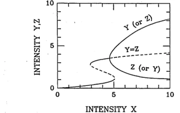
Fig. 2. Steady-state bistable response of the cavity: cavity

in-tensity components Y = Iu+12 and Z = Iu_12 versus the input

intensity component X = S2 calculated for A = 3. The dashed (solid) curves represent unstable (stable) steady-state solutions.

algebraic equations: Ad. ap-eld

ier

ase cur his ion Vs. ien ate .ry-,r). ant are ate (5) By introducing Eq. (5) into Eq. (4), we obtain the fol-lowing two coupled PDE's:

iaU+_ 77 a2U+ +(I1-B U12 1

+ B

_2

az 2 at2 +(2 Iu+I+ 2 2 u )I

+ i(l + iA)u+

- iS = 0, (6a)

.au

_

a2U~

(1

-B U_2 1

+B

IU+12

az 2 at2'+(2 u1 + 2 2U)

+ i(l + iA)u- - iS = 0,

(6b)

where we introduce new dimensionless variables such that the distributed loss coefficient 02/2 in Eq. (4) is reduced to one. We set the new distance z (02/2s) = Z"(02/2L) (the integer values of the variable ZIL = 2z/02

represent the number of circulations in the cavity), the time t r0/(2s) 2 = TO/(21,3" IL)"2, the field amplitudes

u_ q±(2s)S2/0= E±(2yL)"2_{/0, the pump amplitude} S qi(88)"2/02 = 2Ej(2yL)12/02, and the detuning A =

20/02. The set of coupled PDE's in Eqs. (6) describes the dynamics of the MI laser including polarization effects in the case of negligible linear birefringence and in the good-cavity limit.

Let us first consider the cw steady-state solutions of Eqs. (6). By taking the square modulus of Eqs. (6) with a/az = a/at = 0 and introducing the dimensionless in-tensities of the circular polarization modes, say, Y =

Iu+12 and Z = Iu-12, we obtain the following two coupled

[l+

- 1-By

[1+

1 BZB

2

-B ) Jx

- +B

Y)Z=X,

(7a) (7b)

where X = S2is the intensity of the input circular compo-nent (that is, the total input intensity is 2S2). The solu-tion of the third-order polynomial of Eqs. (7) yields the cw steady-state transmission characteristics Y(X) and Z(X) of the fiber cavity. Henceforth let us focus our attention on the case of an electronic nonlinearity mechanism (for example, in a glass fiber), where B = 1/3. The extension of our results to different values of B is immediate and does not qualitatively change the phenomena that we are going to describe here. By subtracting Eq. (7b) from Eq. (7a), we obtain the relation between Y and Z:

(Z

- y)[(y2 + yZ + Z2)/9 -

2A(Y

+ Z)/3

+(1 + A2)] = 0. (8) The first factor yields a symmetric solution Y = Z (that is, a+ = u-). This solution corresponds, for any input power level X or cavity detuning A, to a wave that is linearly polarized along, say, the x axis [by definition, we choose thex andy components of the field as u, (u+ + u-)/(2)"2 and uy (+ - u-)/i(2)"2, respectively]. By substituting Z = Y into one of the Eqs. (7), we obtain the usual scalar transmission characteristic of the resonator:

y3

-

2y

2

+ (1 + A

2

)y = X.

₍₉₎

A bistable transmission occurs whenever A > (3)1/2.1,3,4 Recall that both the lower and the higher positive slope branches of a bistable input-output characteristic Y =

Y(X) are stable with respect to cw perturbations, whereas

the negative slope branch {that is, [2A - ( 2 - ₃) 12]/ ₃ <

Y < [2A + ( 2

- 3)112/3]/3} is unstable; see Fig. 2}. On the other hand, the solutions of the second-order polynomial between the square brackets of Eq. (8)

corre-- I I I I I

I-.

/Z

ry

--~~~~~

By z

(or

I

I--

I =

spond to steady-state solutions that are not linearly polar-ized (that is, Y # Z). Therefore Eq. (8) demonstrates the existence of a polarization-induced symmetry breaking between the two circularly polarized modes of the field in the cavity. As can be seen by the transmission curve in Fig. 2 (here, A = 3), symmetry breaking appears as a pitchfork bifurcation of the linearly polarized (that is, symmetric) solution. At the bifurcation point, the linearly polarized solution exchanges its stability (with re-spect to cw perturbations) with two new stable elliptically polarized solutions, with same ellipticity and opposite handedness. By setting to zero both factors of Eq. (8), we easily obtain the following values of the intensity of the circular components at the symmetry-breaking bifurcation points:

In terms of its complex circular polarization compo-nents, the cw steady-state solution of Eq. (6) that is linearly polarized along the x axis (that is, symmetric with respect to the two circular components) reads as

= u = Us = S[1 + i(A - U₈2)]-1. Let us consider a

periodic perturbation to this eigensolution of the form u±(z, t) = Us + a,(z)cos fit. (11)

By inserting Eq. (11) into Eqs. (6), we obtain the following linearized equations for the perturbation amplitudes a±:

.a

a+ 77 2

+

az

K

2

i -

A + 3 -2 Uli2a+/

Y, = Z+ = 2A + (A2 - 3)1/2 (10) Equation (10) shows that polarization symmetry breaking requires A Ž (3)2, which in turn implies a scalar bistable response. In this asymmetric (bifurcated) regime, the transmission curves Y(X) and Z(X) are easily obtained by the combination of Eq. (8) and Eqs. (7). As can be seen from Fig. 2, at relatively low pump intensities X the cavity transmission curve exhibits the usual scalar bistable cycle where Y = Z. On the other hand, at the pump power level X(Y2) =X(Z2), such that Y_ = Z- = 2A - ( 2 - 3)1/2, the polarization symmetry is broken. Consequently, for pump power levels X > X(Y-) the polarization state of the field in the cavity switches from the unstable linearly polarized state to either one or the other of the two stable elliptical polarization states. As the pump intensity in-creases to the level where X(Y+) = X(Z+), such that

Y+ = Z+ = 2 + (A2 - 3)1/2 (this second bifurcation point

is not shown in Fig. 2), the two stable elliptical branches merge with the linearly polarized solution that remains the only (stable) steady-state solution for any X > X(Y+). Polarization symmetry breaking in the optically bistable response of nonlinear ring resonators was previ-ously reported in numerical calculations of the nonlinear cavity transmissions on the basis of a two-dimensional version of the Ikeda map.'8 A formally analogous effect appears whenever a nonlinear Fabry-Perot resonator is subjected to two incident oblique beams.1 9 In that case the symmetry breaking induces an asymmetry between the transmitted intensities of the two beams. The elliptically polarized steady-state nonlinear eigen-solutions are a nontrivial consequence of the cavity feedback mechanism. In fact, as is well known, in the absence of the cavity the only eigenpolarizations of an isotropic nonlinear medium are linearly or circularly polarized waves.'7 Polarization symmetry breaking in the cavityless nonlinear propagation may arise only in the presence of linear or nonlinear asymmetries, such as for linear birefringence. 2 0

So far we have considered the steady-state response of the nonlinear cavity and its stability against cw pertur-bations. However, the presence of chromatic dispersion leads to instabilities involving the development of time-periodic perturbations of the steady-state solutions (that is, MI's). In what follows we investigate the modula-tional stability of the (linearly polarized) cw solutions in the bifurcation diagram of Fig. 2.

+

21U

2

Ia- +U(2a+

\2

+

2 a_

2/

aa + 772 az 2

=

is)

(12a) i A + 3 - B IUa12)a-1 +B +U.2 ____ -____B = S

+

2

U

+ s

\2 2 (

2 a + 2 a+*=iS.

(12b) When looking for exponentially growing solutions [that is, a exp(Az)], we obtain from Eqs. (12) and their complex conjugates a system of four algebraic equations

in a, and (a,)*. The resulting characteristic polynomial

yields four eigenvalues Ai(i = 1, .. , 4), among which the following two are potentially unstable (that is, A with a

positive real part):

Al

=

-1

+

[4(A

- 77fl2

/2)Y

-

(A

-7

t

fq

2/2)2 - 3y2]/2

(13a)

A

2=-1

+

[

4 (A

- 77

fl

2

/2)Y

-

(A -

/2

]

(13b)

where we have set B = 1/3 in Eqs. (12). Equation (13a) coincides with the dispersion relation obtained in the purely scalar analysis of the ring cavity.34 In fact, the eigenvector associated with Al is, as one would expect, linearly polarized along the x axis (that is, a+ = a-).

In other words, the perturbation grows parallel to the linearly polarized circulating (and pump) field in the cavity. For convenience, let us briefly recall the main results of the scalar MI (SMI) analysis of Refs. 3-5. From Eq. 13(a), we obtain that Al is positive whenever Q_2 <

fQ2

< +2

and

[+2 =

2

₇

(A

-

2Y)

+

2(y

2 - 1)1/2.

From

this condition we may easily draw the regions in the (A - Y) plane, where SMI at a finite frequency detuning prevails (that is, it has a larger peak gain per unit length) over the cw instability of the negative slope branch of the bistable response. As can be seen from Fig. 3, in the anomalous dispersion regime ( = -1) SMI occurs whenever either Y > 1 (if A c 2) or Y > A/2 (if A > 2), whereas in the normal dispersion regime ( = + 1) SMI

450 J. Opt. Soc. Am. B/Vol. 11, No. 3/March 1994 6 5 Cn) z 3 LU Z _w2 -1 0 i- 1rl- SMI,PMI / =-1 SN i--+1 stable / =+1 PN , R=-1 SMI / . - =+1 stable T--1 stable 1=+1 stable I I I I I I I 1 2 3 4 5 6 CAVITY DETUNING A

which corresponds, in physical units, to the following expression for the sideband detuning:

f2max = [ 7(2/L - 2yP./3)/II`]j" 2/21T. (15b)

=-1 stable In a manner similar to that of the scalar case that we

have reviewed above, we may determine for what range of physical parameters PMI prevails over the competing

l l l cw spatial instability of the steady-state solutions. As 7 8 9 10 shown in Fig. 3, in the anomalous dispersion regime PMI

occurs whenever Fig. 3. Regions of MI in the plane of parameters Y - A for both

normal ( = 1) and anomalous (77 = -1) dispersion regimes.

Y > 3

for A 2, occurs whenever 1 < Y < A/2 (if A > 2). Peak SMI gain

Almax = Y - 1 is obtained at the optimum sideband detun-ing from the pump filmax = [2_{7 7}(A - 2Y)]"2. In physical

units, this expression corresponds to the frequency fimax = [-7(20/L - 2yP.)/If3" 1"]/2/2ir, where P. is the power in watts of the linearly polarized pump in the cavity. At the bifurcation point ( that is, for an input power such that the steady-state solution turns out to be modulationally unstable), the eigenvalue A(fl) crosses the imaginary axis at the origin. In other words the bifurcation is real: the absence of an imaginary part of the eigenvalues entails the absence of longitudinal oscillations that accompany MI in the conservative (i.e., cavityless) case.2_{' In} con-trast with the cavityless MI, cavity SMI may also occur in the normal dispersion regime because the cavity phase detuning A permits the phase matching of the four-photon interaction between the steady field and its sidebands.4

Let us consider now the second bifurcation that is char-acterized by the dispersion relation A2(4) in Eq. (13b). The expression for A2reduces to that of Al when we simply

rescale the intensity Y by a factor of 1/3. This result is a direct consequence of the 1:3 ratio between orthogonal and parallel components of the nonlinear susceptibility in silica (that is, B = 1/3). Moreover, like Al, A2 also is

always real and crosses the imaginary axis at the origin. We may then expect that, in analogy with the scalar case, this second real bifurcation will also lead to the formation of time-periodic stationary dissipative structures. The main difference is that the eigenvector that corresponds to A2is linearly polarized along the y axis (that is, the cir-cular components are antisymmetric, so that a+ = -a-).

Therefore polarization MI (PMI) leads to the growth of perturbations that are orthogonal with respect to the steady-state field in the cavity. An interesting question arises as to whether the time-periodic, spatially station-ary dissipative structures that develop from the initial weak modulation also maintain their orthogonal polar-ization in the nonlinear regime of strong pump depletion. The maximum growth rate of the orthogonally polarized PMI sidebands is

A2ma = Y/3- 1. (14)

The gain is obtained at the optimum modulation fre-quency

Q2max = [2₇₇(A - 2Y/3)]'-2, (15a)

Y > 3A/2 for A > 2. (16a)

In the normal dispersion regime however, PMI occurs whenever

3 < Y < 3/2, with A > 2. (16b)

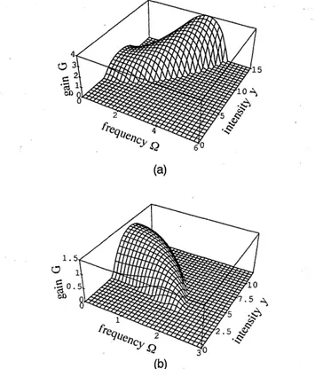
In summary, Fig. 3 displays the domains of SMI and PMI in the (A, Y) plane. Regions exist in which both SMI and PMI may coexist. In this case the SMI, gen-erally speaking, has a higher peak gain, and therefore it is expected to prevail. However, as we shall see in Section 3, the numerical solutions of Eqs. (6) show that a particularly complex dynamics may appear whenever both instabilities are present.

In Fig. 4 we show the dependence of the PMI gain [that is, the growth rate of the orthogonal perturbation, which is given by G = Re(A2) > 0] on the modulational frequency Q2 and intensity Y in either the anomalous [Fig. 4(a)] or the normal [Fig. 4(b)] dispersion regime, respectively, for a fixed value of the detuning, A = 4.

As can be seen in Fig. 4(a), in the anomalous dispersion regime PMI instability occurs for any value of the inten-sity Y that is larger than a given threshold. However, at relatively low intensities the gain curves have a peak for Ql = 0. Because a positive growth rate at Ql = 0 means that the symmetric steady-state solution in the bifurcated domain [that is, for 2A - (A2 - 3)1/2 < Y < 2 + ( 2

-3)1/2] is unstable with respect to cw perturbations, this cw

instability is expected to prevail when we are close to the threshold for PMI. On the contrary, at intensities that are larger than the threshold intensity in Eq. 16(a) (for example, Y = 6 in Fig. 4), maximum gain is obtained at the finite frequency detuning of Eq. (15a).

On the other hand, Fig. 4(b) shows that in the normal dispersion regime PMI builds up only within a limited range of intensities Y. The maximum gain at a nonvan-ishing frequency detuning is only obtained near the lower intensity threshold [see Eq. (16b)].

In analogy with the case of SMI in a cavity,3_'4 the feedback mechanism is essential for explaining the occur-rence of PMI in all the parameter regions of Fig. 3. In fact, in the cavityless propagation the exponential growth of orthogonally polarized sidebands only occurs in the normal dispersion regime.""'6 The physical reason for the occurrence of PMI also in the anomalous dispersion regime is that the cavity detuning shifts the

intensity-II

=- stable q=+1 SMIPMI

3 _ I

on:

(a)

(b)

Fig. 4. Dependence of the PMI gain on the sideband and the steady-state intensity components Y for a cavi

A = 4 and a fiber operating in (a) the anomalous regime ( = -1) and (b) the normal dispersion regin

dependent three-wave mixing phase-matching condition between the steady-state field and the sidebands. By writing the linearized equations for the y-polarized side-bands in which we may decompose the perturbing field

ay a/(2)'/2 = -a-/(2)1/2 in terms of the new variables

Ay,+l -af, exp[-i(i - 77Q2/2 -

A

+ (1 - B)IUoI2]

(here ay, ±n denote the Stokes and anti-Stokes components of the perturbation, that is, ay,n = ay,+n ay/2), we obtain, from Eqs. (12),

-i aY 2 U0X2A + exp(-iAkz), (17a)

a______ = B ( o

a z =2 (Uo)

2

A3

, ,ly exp(+iAkz), (17b)

where Uox = (2)1/2U8 is the x-polarized steady-state solu-tion (that is, IUOX12 = 2Y) and Ak = 2(77(12/2 - A + (1

-B)IUoxI2). From Eqs. (17), we can immediately verify that the phase-matching condition Ak = 0 (with B = 1/3) corresponds to the optimum frequency of Eqs. (15).

We may also provide a simple physical interpretation of the threshold condition Y > 3 in inequalities (16), which is valid in the normal dispersion regime. Indeed, in physical units, this condition reads as yP/6 > 02/2L,

where Px = 21E+12 = 21E- 2 is the power in watts of the linearly polarized steady-state field. Now, yPx/6 is the PMI gain of sidebands that are orthogonal to a wave that propagates in an isotropic fiber in the normal dispersion

regime,16 whereas 02/2L is the loss per unit length that is experienced by the cavity field through its multiple

passes through the coupler. Therefore the condition Y > 3 is the usual intensity threshold condition of a laser cavity.

3. PULSE PATTERN FORMATION PROCESS

The linear stability analysis of the steady-state solutions [Eqs. (7) and (8)] of the coupled NLS [Eqs. (6)] permits a simple characterization of the polarization dependence of the modulational gain of an isotropic MI laser. In this section we support the predictions of the linearized analysis with the direct numerical integration of Eqs. (6) and with initial conditions of the type of Eq. (11). This approach allows us to determine the polarization char-acteristics and the stability of the emitted pulse trains and naturally takes into account the presence of pump depletion. Moreover, as we shall see, the numerical analysis is essential for determining the characteristics of the pulses at the laser output in the cases in which there is competition between SMI and PMI.

We solved Eqs. (6) by a finite-difference method with periodic boundary conditions in time.2' We used a gener-alization of the integrable discretization of the scalar NLS equation that was introduced by Ablowitz and Ladik.2 2 In our scheme the discretization of the two coupled NLS equations involves the numerical integration of the fol-detuning Q lowing 2N coupled ordinary differential equations: ity detuning

s dispersion

ae (77 = 1).

au+i

77 u' + u+i - 2u÷j

az 2 At2

+ 2B lu1+ + 2 Iu'i 2 u~j+ + U-I-i 2

+ i(1 + iA)u±d - iS = 0, (18)

where (j = 1,... ,N), At = T,/(N - 1), and Tw is the time

width of the computational window. The linear stability analysis of Eqs. (6) that is carried out in Section 2 deals only with the interaction of the pump with the first two contiguous sidebands. On the other hand, in the numerical method we solved Eqs. (6) over the window

T = 2vm/f with m an integer, and we used a grid with up to NT = 256 points in each period 2r/f of the input modulation seed. Because the frequency f of the numerical seed was set to be equal to the peak gain value of Eqs. (15), the computations involve a small number (of the order of m) of linearly unstable Fourier modes and a relatively large (of the order of NT) number of linearly stable modes. By stable and unstable mode we mean that the mode's frequency detuning (1 yields from Eqs. (13) an eigenvalue with positive real part. We have verified in the following simulations that whenever a stable pulse train is emitted from the cavity this result does not depend on the particular choice of the number of the stable or unstable Fourier modes. On the other hand, when an irregular emission is observed, the history of the particular chaotic waveform that is generated may depend on the choice of the number of periods m of the modulation in the computational window. Nevertheless, the chaotic character of the field evolution is not critically associated with the choice of the number of the linearly unstable modes in the discretized version [Eq. (18)] of Eqs. (6).

452 J. Opt. Soc. Am. B/Vol. 11, No. 3/March 1994

We used the initial condition of Eq. (11) for the field, with a+ = -a_ = Us/100. We assumed that the pump was always linearly polarized along the x axis, whereas the time-periodic perturbation was orthogonally polarized along the y axis. The presentation of the numerical results in Figs. 5-10 involves the time variable t' that is scaled in units of the modulation period t = 2/Q, so that, in physical units, the time T reads as T = tf, where f is the actual modulation frequency of the seed [see Eq. (15b)].

The study of the domain of validity of the averaged description [Eqs. (6)] of the evolution of the cavity field that we obtain from the semidiscrete map [Eqs. (1) and (2)] is beyond the scope of this paper. We still need to clarify the influence of the higher-order terms in in the series expansions [Eqs. (3) and (4)] in cases for which the conditions (a)-(c), found before Eq. (3), no longer hold. In what follows we limit ourselves to discussing the behavior of the solutions of the averaged Eqs. (6). We have verified that these solutions can be reproduced by directly integrating the map [Eqs. (1) and (2)], provided that conditions (a)-(c) are verified, namely, that 02 << 1 (that is, the good-cavity limit), 0/7r << 1, and L/Ld << 1. Recall that Ld = /1,"1f 2, where f is the frequency of the modulation that builds up [see Eq. (15b) or its scalar equivalent].

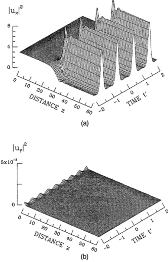
Let us first consider the MI's in the anomalous dis-persion regime (that is, 77 = -1). With reference to Fig. 3, there is a wide region in the (A - Y) plane where SMI occurs yet PMI is forbidden. In this region we suspect that the scalar description does provide a sat-isfactory description of the nonlinear evolution of the field in the cavity even when an orthogonally polarized seed is injected. The numerical integration of Eqs. (6) confirms that this is indeed the case. For example, Fig. 5 shows that a stable pulse train is formed with the same linear polarization of the unstable cw stationary solution even though the perturbing sideband seed is orthogonally polarized. Here the sideband frequency is ( = nlmax = (2)1/2, for Y= 1.5 (that is, IUo12 _{= 2Y = 3) and A = 2.} The only effect of seeding with an orthogonal polarization is that the instability and the pulse pattern take a longer distance (that is, a larger number of circulations in the cavity) to develop.

On the other hand, in the high-power region of the parameter plane of Fig. 3 (that is, when Y > 3 and A < 2Y/3), where PMI competes with SMI, we observed the generation of complex spatiotemporal structures. In principle, whenever PMI is seeded by orthogonal sidebands with the optimum gain frequency ( = l2max

[Eqs. (15)], we might expect that a time-periodic structure whose polarization is orthogonal to the pump would develop. However, for any given values of Y and A, the SMI gain Alma = Y - 1 at the frequency

(

= llmax

is larger than the PMI gain A2ma = Y/3 - 1 at the seed frequency ( = l2max. This means that SMI definitively

prevails over PMI whenever the instability is seeded from noise. Moreover, even if the initial seed at frequency f = limax is strictly zero, a sideband may develop at this frequency in the course of the nonlinear stage of growth of the PMI.

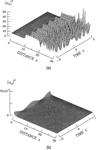
The example of Fig. 6 shows the power evolution in the linearly polarized components of the field, with Y =

Z = 3.2 and A = 1. In this case the linearized stability

analysis predicts the simultaneous presence of both PMI and SMI (see Fig. 3). The initial perturbation is directed along the y axis and has the optimum PMI frequency (1 =

Q2max = 1.5. As can be seen (here the temporal window shows one period of the initial modulation), initially there is a growth of the modulation at the seed frequency in both polarizations. After a distance of approximately z = 30, this polarized wave train loses its stability, and for some distance the field in the cavity oscillates erratically. Finally after some transient chaotic behavior the field is again attracted toward another stable temporal oscilla-tion mode that is linearly polarized along the x axis. The final pulse train is exactly iT out of phase with the initial train, indicating that the two trains may be associated with two nearly symmetric attractors in a finite dimen-sional phase space.5 In conclusion, the larger SMI gain eventually leads, as expected, to a final pulse train that is polarized parallel to the pump. However, this result occurs after a nontrivial succession of transitions through stable and chaotic elliptically polarized attractors.

We found similar behavior when SMI and PMI com-peted in other regions of the parameter space. Although a stable pulse train that is parallel to the pump eventually

1UX12 8 4 _ 4 0 _ 5x0 JU12 IulI _x10 eO '? 6(0 (a) 0 (b)

Fig. 5. Scalar pulse train generation from a modulationally unstable x-polarized cw in the anomalous dispersion regime

(77 = -1). The initial perturbation at the optimum frequency for SMI, Q = limax = (2)1/2, is directed along the y axis. Here we chose Y = Z = 1.5 and A = 2. The time t is measured in

units of the modulation period tp = 2/Ql.

IUX12 40 20 -40 2:

F

4 2 0 u4 60 -(a) 0 e 60 (b)

Fig. 6. Evolution of the linearly polarized components fi modulationally unstable x-polarized cw in the anomalous d sion regime (7 = -1). Here we chose Y= Z = 3.2, A = I the optimum frequency for PMI, (1 = fl2max = 1.5. emerges after the initial transient, an initial chaot ternation between half-period time-shifted and ellipti polarized pulses is observed. As discussed in Refs. this type of coherent low-dimensional chaos also ap] in the scalar treatment of MI lasers whenever the intensity grows larger. The chaos in a diffractive linear Fabry-Perot resonator, where there is an i ular emission in time of spatially transverse cohn structures,5 is analogous.

At relatively large values of the power in the c Y or whenever the instability is seeded at a freqi that is different from the optimum value fl2max for the dynamics in the cavity no longer leads to thE mation of temporal structures that correspond tt stable attractors of the system. On the contrary, a certain number of circulations the cavity tends to in an irregular manner. In this case the pulse tends to be fully polarized along the pump direction. example, Fig. 7 shows the computed evolution of pom the two linear polarization components of the field, the cw x-polarized wave is seeded with an orthol sideband with (1 = 0.5 = (12max/3 (the other param are the same as in Fig. 6). As can be seen, the tem modulation that develops is parallel to the cw bea the cavity. Moreover, the repetition rate of the coincides with the peak SMI gain configuration (In this case fllmax is six times larger than the

frequency (1.) This pulse train is unstable: z > 20 the output intensity from the cavity fluctuates in a chaotic fashion.

In summary, we have shown that, whenever the MI laser operates in the anomalous dispersion regime and the pump is linearly polarized, fluctuations in the polar-ization of the output field only occur during an initial transient. After a certain number of circulations, the polarization state of the laser output remains strictly linearly polarized along the polarization direction of the pump. Moreover, depending on the input intensity, the cavity detuning, and the seed frequency, the emitted pulse trains are either temporally stationary or chaotic.

As we shall see, in the normal dispersion regime of propagation of the fiber (that is, when 77 = 1) the situation may be rather different. In Refs. 3 and 4 we predicted that SMI in a cavity may occur even in the normal dis-persion regime. Numerical solutions of Eqs. (6) confirm the possibility of generating stable pulse trains (temporal dissipative structures) with 7 = 1. On the other hand, Fig. 3 shows that, in contrast with the anomalous disper-sion regime, with normal disperdisper-sion there is a relatively large domain in the A - Y plane where only PMI exists (for Y > 3). However for 1 < Y < 3 (and a proper value

lbt of the detuning) only SMI is observed. Finally, Fig. 3

shows that in the normal dispersion regime SMI and PMI compete only for relatively high values of the detuning

(A > 6). 2 luxl non- a irreg- 4 0° erent avity iency PMI, e

for-)'the

after emit train For rer in when gonal .eters poral .m in train 21max-seed (a) uy12 0 (b)

Fig. 7. Onset of linearly polarized chaos in the cavity for ti

454 J. Opt. Soc. Am. B/Vol. 11, No. 3/March 1994 1U.12 0 'C (a) (b)

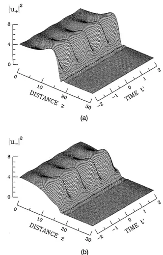
Fig. 8. Stable emission of a pulse train from an unstable cw directed along the x axis in the normal dispersion regime ( = 1). Here Y = Z = 5, A = 4, and Q = Ql2max = 1.155.

Let us consider a situation in which only PMI is present. In this case we expect that PMI would generate pulse trains that are orthogonally polarized with respect to the pump. In terms of counterrotating circularly polarized components of the field, these pulse trains would appear as two 7v out-of-phase identical trains. In Fig. 8 we show the evolution from the steady state of the intensities in the two linearly polarized components of the field that is emitted by the MI laser. The initial seed is again orthogonally polarized with respect to the pump with Y = 5, whereas A 4 and the seed frequency detuning (1 yields peak PMI gain. As can be seen, PMI depletes the x-polarized pump, and the weak, initially y-polarized sidebands grow until a stable train of pulses develops in this polarization. A weaker intensity modulation of the intensity of the x-polarization component is also present. Although the two intensity plots in Fig. 8 show the same modulation period, when we look at the complex amplitudes (or at their power spectra) we find that the weak modulation on the x component results from the parametric growth of the two higher-order sidebands with a frequency detuning from the pump that is equal to 2. This phenomenon arises because the orthogonal susceptibility tensor component X1221 does not couple energy between two orthogonal sidebands with the same detuning (1 from the pump, whereas coupling

between these sidebands and the higher-order sidebands at the detuning 2 is permitted.

Let us briefly point out the feasibility of an experiment involving the observation of a cross-polarized pulse pat-tern as in Fig. 8. In real units the optimum frequency is obtained from Eq. (15b). With the power transmittance 02 = - p2 = 0.04 and the fiber length L = 1 m, we

obtain, for example, that Y = 5 and A = 4 corresponds to a detuning AOX = 0.08 and yP,, = 0.2 (that is, IE 12 4 W for n2 = 3.2 x 10-16 cm2/W, and Aeff = 10- cm2). With

the group-velocity dispersion /3" = 0.035 ps2_{/m at A =} 850 nm, we obtain f2max = 140 GHz. In Fig. 8 we show

the intensity profile of the output pulse train: because a phase shift of v exists between adjacent pulses, the repetition rate of the train that is shown in the figure is equal to T/f2max. Here the ratio, say R, between the full width of the pulses and the repetition rate T/f2max

is equal to 0.625. In the normal dispersion regime the cavity emits a nearly sinusoidal waveform. This result is independent of the precise value of the frequency

f2max-On the other hand, from Figs. 5 and 6 we obtain that in the anomalous dispersion regime R 0.2. In this case, a much larger number of harmonics is generated, which leads to the solitonlike temporal compression of the output pulses in the train. If we want to determine the effect of changing, for example, the input pump power

IEi 12 on the repetition rate (and therefore on the output pulse width in physical units), we should first use Eqs. (7) to find the new value of Y and then use Eqs. (15) to get the peak gain modulation frequency.

In the above numerical example (that of Fig. 8), the dispersion length associated with the pulse train, say

Ld = (Iff2)- = _{1500 m, is much larger than the physical} length of the cavity, which agrees with the assumptions that justify the averaging of Eqs. 1 and 2.-5

In the case of Fig. 8, the generation of a stable pulse train occurs after the normalized distance z = 10, which corresponds to

N = 2z/02= 500 circulations in the ring. The above esti-mates do not critically depend on the precise value of seed power; therefore they should be adequate to demonstrate the feasibility of also observing PMI in a cavity when a modulation builds up from noise at the frequency

fl2max-The growth of pulse trains from PMI in the normal dispersion regime competes with the cw instabilities of the steady-state field (see, for example, Fig. 2, dashed curves). Therefore the dynamic interaction between modulational and dc instabilities may lead to the observation of a modulation-induced switching between different cw stable states of the cavity response. For instance, consider the case Y = 4 and A = 4, so that the initial steady-state solu-tion is on the stable upper branch of the bistable response, before the cw polarization-instability region shown in Fig. 2 [that is, Y < Y(A = 4) 4.4]. In Fig. 9 we show the nonlinear evolution of the intensities of the two circu-lar pocircu-larization components of the field. Figure 9 shows that PMI initially favors the growth of a modulation in the y-polarized cavity field at the seeding frequency. (Here the y-polarized modulation appears as two ir out-of-phase pulse trains.) Although it depletes, the pump intensity

Iu 2 loses its own dc stability. As a result, the field abruptly switches down to the stable lower branch of the S-shaped part of the bistable scalar response (see Fig. 2). In fact, the final intensities of both circular components Haelterman et al.

base 10 Pocl'

Iu+ 2 8 0 (a) 8 0 AIC~~ (b)

Fig. 9. Evolution of the circularly polarized components for the case of modulationally induced downswitching:

Y = Z = 4, A = 4, = 1.155, and a normal dispersion regime.

of the cw field in the cavity are equal to Y = 0.27. This instability is of a dynamic nature in the sense that it cannot be predicted by the linear stability analysis. In fact, the linear stability analysis determines only the transition between cw steady states from the eigenvalues A1(fl = 0) and A2(1 = 0), whose real parts vanish in this case, for which Y = 4 and A = 4 [see also the gain curve in Fig. 4(b)].

In these simulations we also observed a similar be-havior in the purely scalar case (that is, with the seed and the pump both linearly polarized along the same direction) in parameter regions where the linear stability analysis predicts the occurrence of SMI only. In this case switching occurs between the dc stable but modulationally unstable lower branch and the stable upper branch of the bistable loop.

In addition PMI also competes with the dc polariza-tion instability of the cavity steady-state field of Fig. 2. This dc instability leads to polarization switching of the steady cavity response from linear to elliptical stable states [see Eq. (10)]. In Fig. 10 we show the intensities of the circular components from a perturbed x-polarized cw that propagates in the normal dispersion regime. Here Y = 7 and A = 4; Fig. 3 shows that for these input values the linear stability analysis predicts that the peak value of the gain is not associated with PMI. In fact, Fig. 10 shows that, although during an initial transient

a polarization modulation develops, finally a switching to a cw steady state of the field occurs. In this case the initial steady state is polarization unstable [that is,

Y > Y_ (A = 4) - 4.4], and this leads to a final state with

different intensities for the two circular field components. In other words, the stable state of polarization of the field that emerges from the cavity is elliptical, which agrees with the predictions of the multistable response of Fig. 2 and Eq. (10). With the above values for Y and A, the PMI gain curve A₂(() of Eq. (14) has its maximum for

(1 = 0. In other words, the gain of the cw symmetry-breaking instability is larger than the gain of the seeded PMI, which agrees with the dynamics that is numerically observed (see Fig. 10).

Recall that A2(0) characterizes the cw polarization symmetry-breaking bifurcation, that is, A2(0) > 0 for values of Y within the interval [Y-, Y+] of Eq. (11). The analogy between the dc polarization instability and PMI (that is, the instability with respect to finite detuning sidebands) also extends in the nonlinear stage of development of these instabilities. In fact, dispersion shifts the symmetry breaking between two polarizations to a symmetry breaking between two modulated temporal wave trains. A similar effect also arises in the study of period-doubling instabilities in a nonlinear diffractive ring cavity.2 3 lull2 15 10 0 10 (a) lu-12 15 10 _ 5-0 _ 0 (b)

Fig. 10. As in Fig. 9 for modulationally induced symmetry

breaking. Here Y = Z = 7, A = 4, and = 1.

456 J. Opt. Soc. Am. B/Vol. 11, No. 3/March 1994

4. CONCLUSIONS

By means of an averaged model that involves two coupled driven and damped NLS equations, we investigated the dynamics of a MI laser filled with an isotropic nonlinear dispersive medium. We have shown that the inclusion in the description of the state of polarization of the field leads to novel and interesting effects in the dynamic features of the laser.

In the cw limit (that is, whenever dispersion may be neglected) we analytically predicted a symmetry-breaking bifurcation of the linearly polarized steady-state solutions in the upper branch of the bistable response of the cavity. The observable signature of this instability is the

polar-ization multistability of the input-output intensity cavity

transmission characteristics.

By including group-velocity dispersion in the analysis, we showed that PMI may compete with the SMI that is present in the scalar propagation of the field.3 4 We obtained analytical expressions for the PMI growth rates, and we characterized the conditions for the prevalence of either PMI or SMI. In the anomalous dispersion regime of the fiber we found that the dynamics of the field is essentially scalar, although polarization effects may appear during an initial transient stage or may induce a loss of stability of the emitted pulse trains at high powers. On the other hand, in the normal dispersion regime polarization effects may be exploited for the generation of pulse trains. This effect should be easily observable because, as we have seen, the analysis predicts that PMI prevails over SMI in a wide region of the parameter space. In fact, numerical solutions show both the emission of stable pulse trains whose linear polarization is orthogonal to the pump and the modulationally induced switching from an unstable linear to a stable elliptical steady state. From the point of view of the nonlinear dynamics, the structure of the nonlinear ring cavity that we considered here is fully equivalent to that of a nonlinear Fabry-Perot cavity. Therefore our conclusions may be immediately extended to other nonlinear feedback devices. In addi-tion we envisage that the approach of our research may be extended to the analysis of coupled-cavity structures,

such as APM lasers, for which high-power synchronous pumping of a passive fiber cavity is likely to lead to polarization instabilities.

ACKNOWLEDGMENTS

For technical assistance we thank R. Vozzella and R. Chisari. This research was partially supported by a

twinning contract with the Commission of the European Communities on space-time complexity in nonlinear optics, and it was carried out in the framework of the agreement between the Fondazione Bordoni and the Istituto Superiore poste e Telecommunicazioni.

*Permanent address, Service d'Optique Th6orique et Appliqu6e, Universit6 Libre de Bruxelles, 50, Avenue F. D. Roosevelt, CP 194/5, B-1050 Brussels, Belgium.

REFERENCES

1. H. M. Gibbs, Optical Bistability: Controlling Light with

Light (Academic, London, 1985).

2. R. Vall6e, Opt. Commun. 81, 419 (1991).

3. M. Haelterman, S. Trillo, and S. Wabnitz, Opt. Commun.

91, 401 (1992).

4. M. Haelterman, S. Trillo, and S. Wabnitz, Opt. Lett. 17, 745 (1992).

5. M. Haelterman, S. Trillo, and S. Wabnitz, Opt. Commun. 93,

343 (1992); Phys. Rev. A 47, 2344 (1993).

6. D. W. McLaughlin, J. V. Moloney, and A. C. Newell, in Chaos in Nonlinear Dynamical Systems, J. Chandra, ed. (Society

for Industrial and Applied Mathematics, Philadelphia, Pa., 1984); J. V. Moloney, in Nonlinear Phenomena and Chaos,

S. Sarkar, ed. (Hilger, Bristol, UK, 1986), pp. 214-245. 7. G. S. McDonald and W. J. Firth, J. Opt. Soc. Am. B 7, 1328

(1990).

8. B. K. Nayar, K. J. Blow, and N. Doran, Opt. Comput.

Process. 1, 81 (1991).

9. F. Ouellette and M. Pich6, J. Opt. Soc. Am. B 5, 1228 (1988).

10. M. Haelterman, S. Trillo, and S. Wabnitz, Electron. Lett.

29, 119 (1993).

11. E. P. Ippen, H. A. Haus, and L. Y. Liu, J. Opt. Soc. Am. B 6, 1736 (1989).

12. M. Nakazawa, K. Suzuki, and H. A. Haus, IEEE J. Quantum Electron. 25, 2036 (1989); M. Nakazawa, K. Suzuki, H. Kubota, and H. A. Haus, IEEE J. Quantum Electron. 25,

2045 (1989).

13. G. P. Agrawal, Phys. Rev. Lett. 59, 880 (1987).

14. A. L. Berkhoer and V. E. Zakharov, Sov. Phys. JETP 31, 486 (1970).

15. S. Trillo and S. Wabnitz, J. Opt. Soc. Am. B 6, 238 (1989). 16. S. Wabnitz, Phys. Rev. A 38, 2018 (1988).

17. P. D. Maker, B. W. Terhune, and C. M. Savage, Phys. Rev. Lett. 12, 507 (1964).

18. I. P. Areshev, T. A. Murina, N. N. Rosanov, and V. K.

Subashiev, Opt. Commun. 47, 414 (1983).

19. M. Haelterman and P. Mandel, Opt. Lett. 15, 1412 (1990).

20. B. Daino, G. Gregori, and S. Wabinitz, Opt. Lett. 11, 42 (1986); H. G. Winful, Opt. Lett. 11, 33 (1986).

21. S. Trillo and S. Wabnitz, Opt. Lett. 16, 986, 1566 (1991).

22. M. J. Ablowitz and J. F. Ladik, Stud. Appl. Math. 55, 213

(1976).

23. M. Haelterman, Opt. Lett. 17, 792 (1992).