DOTTORATO DI RICERCA
SCIENZE DELLA TERRA
Ciclo XXI
Settore scientifico disciplinare di afferenza: GEO10
Metodologie per il miglioramento delle stime di pericolosità
sismica in Italia
Presentata da:
Dott.ssa LAURA GULIA
Coordinatore
Dottorato
Relatore
Prof. William Cavazza
Prof. Paolo Gasperini
a Paolo, a Stefan e alla mia famiglia grazie!
Introduzione pag. 3
Capitolo 1
La relazione di Gutenberg e Richter pag. 7
Allegati:
1. Testing the b-value variability and its influence on Italian PSHA
2. The influence of b-value estimate in seismic hazard assessment
3. Valutazioni sperimentali di amax provenienti da un albero logico più complesso di quello adottato per la redazione di MPS04
Capitolo 2
Analisi dei cataloghi strumentali regionali europei per
l’individuazione di eventi non naturali pag. 9
Allegati:
1. Detection of quarry and mine blast contaminations in European regional catalogues
2. Alcune tra le analisi non inserite nell’articolo
Capitolo 3
Possibili relazioni tra b-value e meccanismi di
fagliazione pag. 14
3.1 Stato dell’arte pag. 14
3.2 Metodo pag. 19
3.2.1 Dataset pag. 20
3.3 Risultati pag. 27
3.4 Conclusioni pag. 33
4. Conclusioni pag. 35
5. Bibliografia pag. 37
6. Allegati
HALM: a hybrid asperity likelihood model for Italy
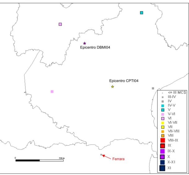
Versione aggiornata al 2007 del catalogo CPTI DBM01: il database delle osservazioni
macrosismiche dei terremoti italiani utilizzate per la compilazione del catalogo parametrico CPTI04
1
Riassunto
In questo lavoro di dottorato sono stati analizzati differenti strumenti impiegati per le stime di pericolosità sismica.
Facendo riferimento alla Mappa di Pericolosità Sismica Italiana MPS04 (Gruppo di Lavoro MPS, 2004), redatta dall’Istituto Nazionale di Geofisica e Vulcanologia (INGV) e adottata come mappa di riferimento per il territorio nazionale ai sensi dell’Ordinanza PCM 3519 del 28 aprile 2006, All. 1b, è stato approfondito il calcolo dei tassi di sismicità attraverso la relazione di Gutenberg e Richter (1944). In particolare, si è proceduto attraverso un confronto tra i valori ottenuti dagli autori della Mappa (Gruppo di Lavoro MPS, 2004) e i valori ottenuti imponendo un valore costante e unico al parametro b della relazione (Gutenberg e Richter, 1944).
Il secondo tema affrontato è stato l’analisi della presenza di eventi di origine non tettonica in un catalogo. Nel 2000 Wiemer e Baer hanno proposto un algoritmo che identifica e rimuove gli eventi di origine antropica. Alla metodologia di Wiemer e Baer (2000) sono state apportate delle modifiche al fine di limitare la rimozione di eventi naturali. Tale analisi è stata condotta sul Catalogo Strumentale della Sismicità Italiana (CSI 1.1; Castello et al., 2006) e sui cataloghi Europei disponibili online: Spagna e Portogallo, Francia, Nord Europa, Repubblica Ceca, Romania, Grecia.
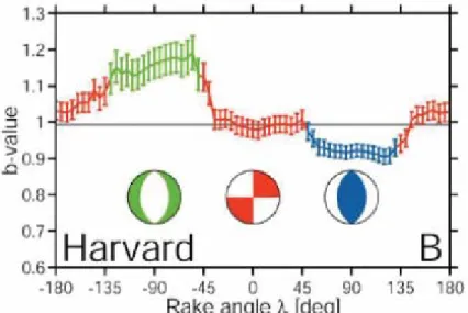
L’ultimo argomento trattato ha riguardato la presunta correlazione tra i meccanismi di fagliazione e il parametro b della relazione di Gutenberg e Richter (1944). Nel lavoro di Schorlemmer et al. (2005), tale correlazione è dimostrata calcolando il b-value su una griglia a scala mondiale raggruppando i terremoti in
2
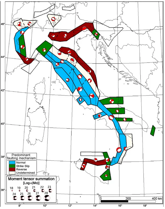
Il principale ostacolo per una applicazione del metodo al territorio italiano è rappresentato dal numero ridotto di terremoti per i quali è possibile avere indicazioni circa il meccanismo focale della sorgente: la correlazione è stata così valutata calcolando il b-value all’interno delle zone sismogenetiche definite per la realizzazione di MPS04 (Gruppo di Lavoro MPS, 2004), alle quali è stato nuovamente assegnato un meccanismo di fagliazione prevalente attraverso la somma del tensore momento.
Sono inoltre allegati lavori altri lavori prodotti nell’ambito della pericolosità sismica.
3
Introduzione
La pericolosità è comunemente definita come la probabilità di occorrenza di un fenomeno in grado di produrre danno. In questa tesi verranno analizzati differenti strumenti impiegati per le stime di pericolosità sismica: i primi due capitoli sono composti da una serie di lavori (due pubblicati e uno sottomesso) mentre l’ultimo capitolo è strutturato in maniera tradizionale.
In particolare, nel primo capitolo verranno illustrate alcune tra le scelte operate per la redazione della Mappa di Pericolosità Sismica Italiana MPS04 (Gruppo di Lavoro MPS, 2004) e confrontate con scelte alternative. La Mappa di Pericolosità Sismica Italiana MPS04 (Gruppo di Lavoro MPS, 2004), redatta dall’Istituto Nazionale di Geofisica e Vulcanologia nell’anno 2004, esprime la probabilità in termini di accelerazione orizzontale di picco (PGA, peak ground acceleration), secondo lo standard europeo EC8, il quale prevede che venga quantificata come probabilità di superamento del 10% in 50 anni -equivalente a un periodo di ritorno di 475 anni-. La mappa è stata elaborata adottando la metodologia probabilistica classica, cioè il modello di Cornell (1968), il quale prevede l’identificazione di aree sismotettonicamente omogenee –definite zone sismogenetiche- all’interno delle quali i terremoti siano equiprobabili nello spazio e il loro rilascio nel tempo sia un processo di tipo Poissoniano (cioè i singoli eventi sono indipendenti tra loro e stazionari nel tempo).
Per elaborare un modello probabilistico di questo tipo sono quindi necessari: • un modello sismotettonico per descrivere le sorgenti;
• un catalogo sismico dal quale ricavare i tassi di sismicità;
• un modello predittivo per le attenuazioni di moto del suolo in funzione della distanza e della magnitudo.
Al fine di esplorare le incertezze di tipo epistemico, con particolare riferimento agli intervalli di completezza dei cataloghi, alla determinazione dei tassi di
4
alternative. In questa tesi di dottorato sono state analizzate le scelte che hanno riguardato il calcolo dei tassi di sismicità e, in particolare, la relazione di Gutenberg e Richter (1944). Motivazioni, metodologie e risultati sono illustrati in Gulia e Meletti (2008) e in uno dei due rapporti tecnici prodotti all’interno della convenzione DPC-INGV ‘Progetti Sismologici e Vulcanologici di interesse per il Dipartimento della Protezione Civile’. Questi lavori sono stati inoltre presentati al First European Conference on Earthquake Engineering and Seismology (1th ECEES,
Ginevra, 3-8 settembre 2006).
Un aspetto affrontato invece nella redazione della Mappa di Sismicità della Svizzera (Giardini et al., 2004), ma poco approfondito in letteratura, è quello della presenza di eventi di origine non naturale nei cataloghi sismici. Nel secondo capitolo viene presentato un articolo (Gulia, 2008), sottomesso alla rivista Natural Hazards, nel quale sono analizzati alcuni tra i cataloghi strumentali regionali europei, tra cui il Catalogo della Sismicità Italiana (CSI 1.1, Castello et al., 2006). La presenza di un elevato numero di falsi terremoti può alterare le stime di hazard: ad esempio, trattandosi di eventi a bassa magnitudo (<3), può portare ad una sovrastima del valore del parametro b della relazione di Gutenberg e Richter (1944) e, in maniera più ampia, rappresenta una fonte di errore per tutti gli utilizzatori dei cataloghi per fini statistici. Inoltre, lo sviluppo, negli ultimi anni, di analisi di pericolosità e forecasting sempre più basate su dati di microsismicità (e.g. Schorlemmer e Wiemer, 2005) comporta la necessità di un dataset completo già a piccole magnitudo: la discriminazione tra sismicità naturale e sismicità generata dall’attività antropica sta assumendo quindi una crescente importanza.
La ricerca di tali eventi è stata condotta attraverso l’applicazione dell’algoritmo di Wiemer e Baer (2000), al quale sono state apportate alcune modifiche.
Nel terzo capitolo viene infine analizzata la ipotizzata correlazione tra i meccanismi di fagliazione e il parametro b della relazione di Gutenberg e Richter (1944) nel territorio italiano e nelle regioni europee per le quali è disponibile una zonazione sismogenetica. Nel lavoro di Schorlemmer et al. (2005), la
5
seguono quelli in un regime trascorrente mentre i valori minori si ottengono per i regimi compressivi. In quest’ottica il parametro b viene definito dagli autori (Schorlemmer et al., 2005) un misuratore dello sforzo (stressmeter), cioè strettamente legato allo stress differenziale. Il principale ostacolo per una applicazione del metodo al territorio italiano è rappresentato dal numero ridotto per i terremoti per i quali è possibile avere indicazioni circa il meccanismo focale della sorgente: la correlazione è stata così ricercata calcolando il b-value all’interno delle zone sismogenetiche, alle quali è stato assegnato un meccanismo di fagliazione prevalente attraverso la somma del tensore momento.
7
La relazione empirica tra frequenza e magnitudo di un terremoto può essere espressa con la legge di potenza descritta nel 1939 da Ishimoto and Iida ma generalmente nota come relazione di Gutenberg and Richter (1944):
Log N (M)= a – b M
dove N è il numero cumulativo degli eventi con magnitudo ≥ M e i parametri a e b sono costanti. In particolare, a è funzione del numero dei terremoti e delle dimensioni dell’area e può quindi fornire una misura approssimativa del tasso di sismicità totale (es. Pacheco et al., 1992; Lopez Casado et el., 1995; Rhoades, 1996; Abercrombie et al., 1996; Bayrak et al., 2002); b, che graficamente rappresenta la pendenza della retta, esprime invece il rapporto tra il numero di piccoli e grandi terremoti. Più semplicemente, il numero di terremoti che avviene in una regione in un dato intervallo di tempo diminuisce in maniera esponenziale all’aumentare della magnitudo: il numero dei piccoli terremoti è cioè molto maggiore rispetto a quello dei grandi terremoti.
Mentre le dimensioni del parametro a sono oggettivamente legate all’intervallo spazio-temporale, il valore del parametro b ha alimentato e continua ad alimentare un fertile dibattito nella letteratura scientifica degli ultimi decenni. Gutenberg e Richter (1944) notarono che, a scala mondiale e per aree molto estese, questo potesse essere prossimo all’unità. Se tale valore fosse invece variabile nel tempo e/o nello spazio descriverebbe il processo fisico come dipendente e controllato da altri fattori, quali, ad esempio, l’eterogeneità della crosta, la cinematica dell’area, la profondità dello strato sismogenetico.
L’argomento verrà trattato con maggiore dettaglio nel capitolo 3.
In generale, trattandosi di una legge di potenza, il processo di generazione dei terremoti è così caratterizzato da invarianza di scala, implicando uguali caratteristiche per piccoli e grandi eventi.
Ai fini della pericolosità sismica, una conseguenza diretta della variabilità del parametro b è nel calcolo dei tassi di sismicità di una determinata regione. Infatti, un b inferiore all’unità indica un numero di eventi a magnitudo alta maggiore rispetto al numero di eventi a magnitudo bassa e viceversa.
8
settembre 2006), viene valutato l’impatto sulle stime di hazard della scelta di un valore fisso e costante per il parametro b attraverso il confronto tra la Mappa di Pericolosità Sismica Italiana (MPS04, Gruppo di Lavoro MPS, 2004), realizzata associando ad ogni zona sismogenetica (Meletti et al., 2008) un differente b, e una mappa ottenuta attraverso la medesima procedura (stesso albero logico e stesse scelte per catalogo, leggi di attenuazione del suolo e zonazione sismogenetica), ma imponendo un b fisso e uguale a 1.
La procedura legata al calcolo dei tassi adottati in Gulia e Meletti (2008) è spiegata in dettaglio nella seconda parte del secondo lavoro allegato (Meletti et al., 2007). Si tratta del rapporto tecnico prodotto all’interno della convenzione DPC-INGV ‘Progetti Sismologici e Vulcanologici di interesse per il Dipartimento della Protezione Civile’ per il Progetto S1- Proseguimento della assistenza al DPC per il completamento e la gestione della mappa di pericolosità sismica prevista dall'Ordinanza PCM 3274 e progettazione di ulteriori sviluppi-, Task 1, Deliverable D5.
59
Testing the b-value variability in Italy and its influence on
Italian PSHA
L. GULIAandC. MELETTI
Istituto Nazionale di Geofisica e Vulcanologia , Pisa, Italy
(Received: April 2, 2007; accepted: May 23, 2007)
ABSTRACT The supposed b-value spatial variability is the central topic of many scientific works dealing with forecast modeling applications or geological correlations. If used for seismicity rate determination, the b-value plays an important role in probabilistic seismic hazard assessment, but how much does it influence the results? In the logic tree approach used for the new probabilistic seismic hazard map of Italy, named MPS04, one of the sources of epistemic uncertainty considered was the procedure for computing seismicity rates. Two alternatives were adopted: 1) to compute the activity rates for each binned magnitude class and 2) to compute a Gutenberg-Richter distribution. In the logic tree branches, where the Gutenberg-Richter distribution was adopted, the corresponding b-value was evaluated for each seismogenic zone: it spans between 0.63 and 2.01. After analysing the b-value variability in the Italian region, this work evaluates the impact of setting the b-value equal to 1 on the results of seismic hazard assessment in terms of PGA and energy release compared to the choices adopted for MPS04.
1. Introduction
The Gutenberg and Richter (1944) relation defines the empirical relationship between frequency and magnitude of earthquakes as
Log N (M) = a – b M
where: N is the cumulative number of earthquakes of magnitude ≥ M; a and b are constants. a depends on seismicity rates; b is representative of the earthquake, size ratio. The authors themselves define b-value equal to 1 on a worldwide scale and for large volumes.
Nowadays the b-value estimation at different scales is the subject of many scientific works, as it may reflect physical properties of the media. There are two main theories:
1. b-value is fixed and equal to 1 (Kagan, 2002): it implies considering the earthquake processes not only to be self-similar but also globally invariant, giving the same characteristics to small and large events;
2. b-value is variable (e.g. Lomnitz-Adler, 1992; Pacheco et al., 1992; Shanker and Sharma, 1998; Schorlemmer and Wiemer, 2005; Schorlemmer et al., 2005; Wiemer and Schorlemmer, 2007): it implies relationships with different tectonic regimes, stress-changes and heterogeneity of the materials.
Many authors pointed out the spatio-temporal b-value variability: some of them in seismic
60
hazard assessment analysis [e.g. Shanker and Sharma (1998) for the Himalayan region], others in earthquake forecasting modeling application [e.g. Schorlemmer et al. (2004a, 2004b) both for California] and others in correlations between b-value and tectonics [e.g. Lopez-Casado et al. (1995) for the Betic Cordillera; Oncel et al. (1996) for the Anatolian fault zones, Turkey; Schorlemmer et al. (2005) for a worldwide correlation between b-value and focal mechanisms]. Bayrak et al. (2002) and Olsson (1999) summarize the state-of-the-art of different b-value estimates in literature; Marzocchi and Sandri (2003) summarize different methods to estimate the b-value while Krinitzsky (1993) highlights the limits of the Gutenberg and Richter (from now on GR) distribution for the application in the engineering of critical structures.
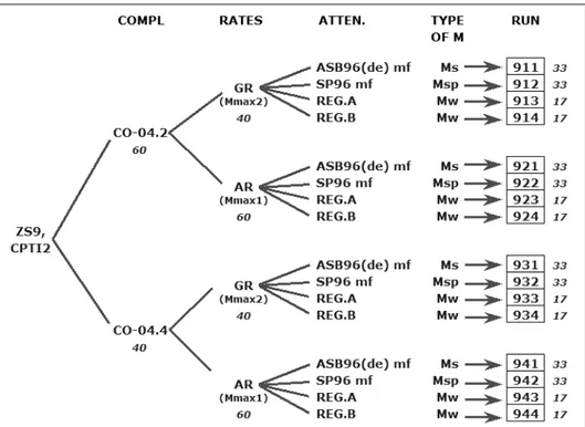
The probabilistic seismic hazard map of Italy (MPS04, MPS Working Group, 2004), recently adopted as the national reference map for planning and design purposes, was elaborated applying a logic tree approach (Fig. 1) which considers two alternative sets of catalogue completeness time-intervals, four ground motion attenuation relationships (see Montaldo et al., 2005) and two different modalities for the estimation of seismicity rates: one uses the GR relation; the other (AR) evaluates independent rates for each binned magnitude class. No alternatives were considered for the seismogenic zonation [ZS9, Meletti et al. (2007). Fig. 2] and for the earthquake catalogue [CPTI04, CPTI Working Group (2004)], since no really epistemic options are available. In all, the logic tree results in 16 branches which have been weighted based on expert opinion as indicated in Fig. 1.
In the eight branches where the GR relation was adopted, the b-value was evaluated for each seismogenic source zone, yielding values in the range from 0.63 to 2.01. Although not explicitly indicated in their technical report, the underlying assumption made by the authors of MPS04 is that the b-value varies as a consequence of different seismotectonic characteristics. Therefore, it should vary from one source zone to the other.
To verify this hypothesis, in the first part of this article we analyse the spatial variability of the b-value in the Italian territory at different scales using different zoning options or a regular grid.
In the second part instead, we test how a b-value always equal to 1 influences the seismic hazard assessment, considering all branches of the logic tree of Fig.1 and the relative weights.
2. Analysis of the b-value spatial variability
The spatial variability of the b-value was analysed using a regular grid (a 16-cell square) with 1° spacing; the square bounds are 34°N, 50°N, 5°E and 21°E (Fig. 3). We use the same catalogue adopted in MPS04, i.e. CPTI04 catalogue (CPTI Working Group, 2004) and the same two sets of completeness time intervals, one historical and one statistical. The catalogue, developed during the processing of MPS04, contains earthquakes with Io≥ 5.5 and it is declustered; only for the Etna volcanic area a lower threshold was adopted. It reports 2550 earthquakes from 217 B.C. to 2002 A.D. in Italy and surrounding regions; moment magnitude spans between 3.92 and 7.41. Fig. 4 shows the distribution of epicenters according to the two completeness time intervals.
A difference with respect to MPS04 is that the completeness intervals were defined for 12 magnitude classes and for each source zone, whereas we chose the completeness time-intervals of one source zone to represent an average completeness for the whole catalogue (Table 1), because a direct correlation between source zones and cells does not exist. We calculated
61
seismicity rates for a 100-year period for each grid cell. In order to evaluate only the impact of the fixed b-value, we chose to use the same procedure adopted in MPS04, including the least squares method for seismicity rate determination, even if we are aware of its limits, as described by McGuire (2004). In the CPTI04 catalogue, 1471 earthquakes are consistent with historical completeness and 1113 earthquakes with the statistical one.
The b-value variability was evaluated through two methods: 1) by a regular subdivision of the grid in the cells and 2) by grouping the cells depending on geographical neighbourhood. In this work, we limited our analysis to the observation of the variability, without investigating its causes (e.g. a different number of earthquakes, area dimensions or geological characteristics).
Fig. 1 - Logic tree adopted in MPS04 (MPS Working Group, 2004). The number close to each epistemic alternative represents its weight.
4.76 ±0.115 4.99 ±0.115 5.22 ±0.115 5.45 ±0.115 5.68 ±0.115 5.91 ±0.115 6.14 ±0.115 6.37 ±0.115 6.60 ±0.115 6.83 ±0.115 7.06 ±0.115 7.29 ±0.115 Historical completeness 1871 1871 1700 1700 1530 1530 1300 1300 1300 1300 1300 1300 Statistical completeness 1910 1871 1871 1700 1700 1530 1530 1300 1300 1300 1300 1300
Table 1 – Time completeness intervals of the CPTI04 catalogue used for the analysis of the b-value variability in the Italian territory.
62
2.1. Regular subdivision of the grid
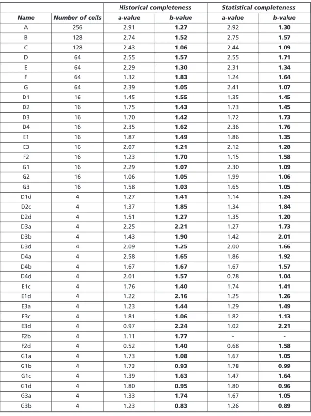
The whole grid (named A), which contains 256 cells, was divided into smaller areas with a decreasing number of cells: 1) half the number of cells (Fig. 3b), 2) the fourth part (Fig. 3c) and 3) the sixteenth part (Fig. 3d). The areas with a-value greater than 0.50 were subdivided further. Areas containing 64 to 256 cells are indicated by capital letters while smaller areas (16 cells) with capital letters and numbers and the smallest areas (4 cells; Table 2) with capital letters, numbers and small letters.
Table 2 sums up the a-values and b-values obtained for successive grid subdivisions: 39 areas according to the historical completeness and 38 areas according to the statistical one, have a statistically firm number of events. The b-value for the whole grid is 1.27 according to the historical completeness and 1.30 according to the statistical completeness (from now on the first b-value will refer to historical completeness and the second to the statistical one). 36 areas out of 39 and 35 out of 38 (Table 2) have a b-value greater than 1 and there is no correlation between the two parameters of the GR relation: the b-value is independent of the number of events (Fig. Fig. 2 - ZS9 seismogenic zonation, redrawn from Meletti et al. (2007).
63
Historical completeness Statistical completeness
Name Number of cells a-value b-value a-value b-value
A 256 2.91 1.27 2.92 1.30 B 128 2.74 1.52 2.75 1.57 C 128 2.43 1.06 2.44 1.09 D 64 2.55 1.57 2.55 1.71 E 64 2.29 1.30 2.31 1.34 F 64 1.32 1.83 1.24 1.64 G 64 2.39 1.05 2.41 1.07 D1 16 1.45 1.55 1.35 1.45 D2 16 1.75 1.43 1.73 1.45 D3 16 1.70 1.42 1.72 1.73 D4 16 2.35 1.62 2.36 1.76 E1 16 1.87 1.49 1.86 1.35 E3 16 2.07 1.21 2.12 1.28 F2 16 1.23 1.70 1.15 1.58 G1 16 2.29 1.07 2.30 1.09 G2 16 1.06 1.05 1.99 1.06 G3 16 1.58 1.03 1.65 1.05 D1d 4 1.27 1.41 1.14 1.24 D2c 4 1.37 1.85 1.34 1.84 D2d 4 1.51 1.27 1.35 1.20 D3a 4 2.25 2.21 1.27 1.73 D3b 4 1.43 1.90 1.42 2.01 D3d 4 2.09 1.25 2.00 1.66 D4a 4 2.58 1.65 1.86 1.92 D4b 4 1.67 1.67 1.67 1.57 D4d 4 2.01 1.57 0.78 1.04 E1c 4 1.76 1.40 1.74 1.41 E1d 4 1.22 2.16 1.25 1.26 E3a 4 1.23 1.44 1.29 1.49 E3c 4 1.81 1.06 1.82 1.13 E3d 4 0.97 2.24 1.02 2.21 F2b 4 1.11 1.77 - -F2d 4 0.52 1.40 0.68 1.58 G1a 4 1.73 1.08 1.67 1.05 G1b 4 1.73 0.93 1.78 0.99 G1c 4 1.39 1.63 1.47 1.64 G1d 4 1.80 0.95 1.80 0.96 G3a 4 1.33 1.74 1.67 1.05 G3b 4 1.23 0.83 1.26 0.89
Table 2 - The a-values and b-values obtained for whole grid and for grid subdivisions according to historical and statistical completeness time intervals; each grid subdivision area is characterised by name and number of cells. The areas missing are those where there is a small number of earthquakes.
64
Fig. 3 - The regular grid (a 16-cell square with a 1° spacing) used for the analysis of the b-value variability; the square bounds are 34° N, 50° N, 5° E and 21° E. a) for the whole grid. Regular subdivision of the grid: b) half the number of cells; c) the fourth part; d) the sixteenth part; e) the sixty-fourth part; these areas have an a-value greater than 0.50.
a
b
c
d
65
5). For both completenesses the b-value shows a wide variability and values very different to 1.
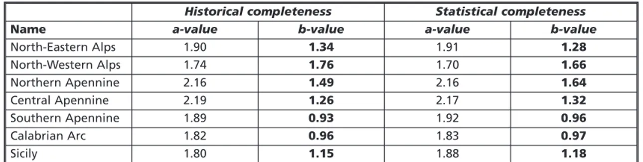
2.2. Geographical grouping of the cells
The cells were grouped by a rough tectonic criterion (Fig. 6): north-eastern Alps (cells 51-52-53-67-68-69-83-84), north-western Alps (cells 54-55-56-57-70-71-72-73), northern Apennine (cells 85-86-87-88-102-103-104), central Apennine (cells 105-119-120-121-136-137), southern Apennine (cells 122-138-139-140-153-154-155-156), Calabrian Arc (cells 171-172-173-187-188-189) and Sicily (cells 184-185-186-200-201-202-203-216-217-218-219). Table 3 shows the Fig. 4 - Maps of the epicenters in CPTI04, according to the historical completeness time interval (a) and to the statistical completeness time interval (b), showed in Table 1.
a
b
Historical completeness Statistical completeness
Name a-value b-value a-value b-value
North-Eastern Alps 1.90 1.34 1.91 1.28 North-Western Alps 1.74 1.76 1.70 1.66 Northern Apennine 2.16 1.49 2.16 1.64 Central Apennine 2.19 1.26 2.17 1.32 Southern Apennine 1.89 0.93 1.92 0.96 Calabrian Arc 1.82 0.96 1.83 0.97 Sicily 1.80 1.15 1.88 1.18
66
results: in the Alps, the northern Apennines, the central Apennines and Sicily, the b-value is greater than 1 and varies from 1.15 to 1.76; in southern Italy and Calabria it is less than 1 (from 0.93 to 0.97). These values match the MPS04 b-values (Table 4) reasonably well: greater than 1 for northern and central Italy and for Sicily, less than 1 for southern Italy.
The above analyses, based on different kinds of subdivisions of the Italian territory (cells or Historical Completeness Statistical Completeness
SSZ in ZS9 MPS04 b
value MPS04 Test 1 Test 2
MPS04 b
value MPS04 Test 1 Test 2
901 1.18 3.15 2.96 4.04 1.26 4.63 5.82 5.80 902 1.26 6.22 9.13 6.59 1.05 6.62 6.65 6.73 903 1.26 2.69 4.28 2.87 1.05 2.43 4.43 3.42 904 1.12 1.44 4.50 2.41 1.32 1.36 5.09 2.18 905 1.06 31.19 49.82 30.43 1.12 38.23 60.17 40.37 906 1.14 8.70 21.37 8.05 1.70 6.35 18.62 13.58 907 1.71 2.02 3.53 2.17 1.48 2.33 5.51 3.27 908 1.91 3.01 8.06 5.47 1.67 3.07 8.03 5.13 909 1.27 1.90 2.65 3.70 1.38 2.72 4.49 4.13 910 1.12 6.79 10.28 7.09 1.06 6.40 7.31 6.59 911 1.47 1.27 3.81 2.32 1.33 1.77 4.93 3.26 912 1.35 5.58 5.68 4.40 1.32 4.92 4.94 3.89 913 1.80 5.60 18.09 6.16 1.53 7.56 13.47 8.75 914 1.33 6.93 15.95 6.50 1.23 9.47 11.03 9.32 915 1.34 15.72 49.81 26.37 1.36 22.34 59.66 23.76 916 1.96 2.18 4.42 3.18 1.58 3.09 4.99 4.49 917 1.04 8.81 6.66 6.61 1.01 11.01 8.42 8.12 918 1.10 15.24 16.99 11.79 1.11 19.34 19.40 15.31 919 1.22 17.33 28.62 18.79 1.39 18.04 33.53 20.13 920 1.96 6.40 12.02 9.06 1.58 7.75 10.99 8.31 921 2.00 6.58 14.95 5.50 2.01 6.18 13.56 7.36 922 2.00 1.96 3.02 1.81 2.01 2.37 2.02 2.28 923 1.05 104.10 179.30 105.45 1.09 98.30 163.22 103.62 924 1.04 30.85 40.42 31.17 1.06 30.97 44.78 31.42 925 0.67 27.35 14.28 15.84 0.75 29.95 19.40 19.46 926 1.28 2.26 4.86 2.82 1.38 2.74 5.52 3.33 927 0.74 183.67 100.74 120.34 0.72 179.08 86.95 115.32 928 1.04 3.53 2.79 2.82 0.66 4.76 2.74 3.35 929 0.82 250.84 144.00 182.45 0.79 259.59 114.47 189.39 930 0.98 21.99 23.21 21.59 0.89 26.12 16.87 23.64 931 0.63 24.81 9.54 11.93 0.63 24.81 9.54 11.93 932 1.21 5.15 10.43 5.17 1.08 7.19 8.08 5.15 933 1.39 8.75 9.80 6.87 1.24 11.37 10.70 12.05 934 0.96 3.13 3.85 2.84 0.93 3.07 3.48 2.77 935 0.72 80.82 32.46 45.97 0.69 111.96 35.50 56.23 936 1.63 2.54 2.46 2.04 1.22 2.90 2.13 2.12 Total energy 910.51 874.74 732.61 980.78 836.42 785.93
Table 4 - Energy release (value x 1013 joule) in each seismogenic source zone for historical and statistical completenesses evaluated from the seismicity rates normalized to 100 years in MPS04, in the test 1 and in the test 2 and adopted b-values in MPS04.
67
Fig. 5 . Relation between the
b-value and the a-value (log
of the total number of earthquakes) in the whole grid and in the smaller areas, according to the historical completeness (Co.04.2) and the statistical one (Co.04.4).
Fig. 6 - Tectonic grouping of the cells: north-eastern Alps, north-western Alps, northern Apennines, central Apennines, southern Apennines, Calabrian Arc and Sicily.
68
areas or source zones) highlight the high variability of the b-value: the use of a constant value seems to be unreal for the Italian region. Anyway, in order to understand if the choice of a fixed b-value is significant or not with respect to the seismic hazard assessment, we performed two different tests in the following.
3. Testing b-value equal to 1
The impact of a b-value fixed to 1 was evaluated through the re-processing of the whole logic tree used in MPS04 (Fig. 1). We fixed the b-value equal to 1 in all the GR branches and selected two alternatives for the determination of the a-value, that is the cumulative number of events:
i) Test 1: the same a-value estimated in MPS04 was adopted, i.e. the same total number of events;
ii) Test 2: re-evaluating the a-value in each source zone with the least squares method using the fixed b-value. As a consequence the total number of events changes with respect to MPS04: more if the original b-value was less than 1; less in the opposite case.
As in MPS04, whenever the maximum magnitude is assumed higher than the maximum historical earthquake, the corresponding seismicity rate is determined extrapolating the GR relation.
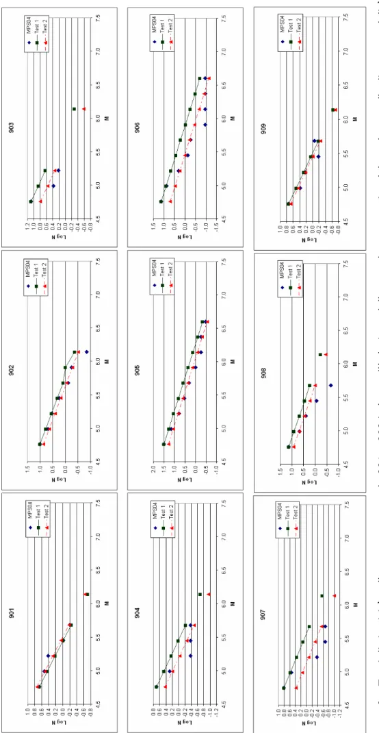
Fig. 7 compares the three different fitting procedures (GR distribution in MPS04; GR distribution according to the test 1 approach; GR distribution according to the test 2 approach) applied to the observed rates (i.e. cumulative number of events per magnitude bin) represented by the blank diamonds. The comparison is shown for two seismogenic source zones (SSZ) where the b-value computed in MPS04 was respectively greater than 1 (SSZ 915) and less than 1 (SSZ 935).
SSZ 915 (Fig. 7a): test 1 has the same total number of events as the MPS04 but a different
distribution among magnitude classes. In particular, the number of large earthquakes increases and, consequently, the number of small earthquakes decreases. Test 2 leads to a new a-value, Fig. 7 - Frequency-magnitude distribution according to the MPS04 (blank diamonds for AR rates and blank circles for GR rates) and the two tests (triangles for test 1 and squares for test 2): a) source zone with an original b-value >1 (SSZ 915); b) source zone with an original b-value <1 (SSZ 935).
69
smaller with respect to that of MPS04: the number of large earthquakes increases, while the number of small ones decreases much more than in test 1. The seismicity rates are smaller in test 2 than in test 1 (less earthquakes are forecast).
SSZ 935 (Fig. 7b): in test 1 the number of large earthquakes decreases and consequently the
number of small earthquakes increases with respect to MPS04. In test 2, the new a-value is greater with respect to MPS04, hence the number of large earthquakes decreases, while the number of the small ones increases. Test 2 presents higher seismicity rates than test 1 (more earthquakes are forecast).
3.1. Single point and single branch analysis
Two seismic hazard maps representing PGA with 10% probability of exceedance in 50 years for hard ground sites were computed following the logic tree and the procedure described previously. In order to compare all elaborations with MPS04, the same regular spaced grid and the same software were used.
A weighted median (50thpercentile) values as well as the 84thand 16thpercentiles were obtained
Fig. 8 - Single branch PGA values for MPS04, test 1 and test 2: a) SSZ 915; b) SSZ 935. In the lower part of the graphs the median value and the variability (expressed by the 16th and 84th percentiles) are superimposed and represented by a symbol and bars.
a
70
by combining the 16 individual maps in a post-processing stage as done in MPS04.
To understand how different options influence the results, we first selected and analysed two localities and compared each branch of the logic tree and the three percentiles. Results are shown in Fig. 8: for both localities, the single values of each branch in the tests are reported; the X-axis is the PGA value and the Y-axis is the relative weight of the branch. The percentiles, according to MPS04 and the two tests, are reported too. Of course, the results for the 8 unmodified branches are the same.
Fig. 8a shows the results obtained for a site in a source zone site in the northern Apennine (SSZ 915) where the b-value in MPS04 is greater than 1. The distribution of the points representing the 16 branches is obviously different in the three approaches. In test 1, higher values and a wider dispersion correspond to a higher median estimate and a greater variability. In test 2, on the contrary, the median is quite similar to the MPS04 estimate.
Fig. 8b shows the results obtained for a locality in a source zone in southern Italy (SSZ 927) where the b-value in MPS04 is less than 1. For both tests the values obtained for single branches are lower than the MPS04 estimates and the median results are approximately 10% lower. Again in test 1 the variability increases; in test 2, it decreases slightly even if the median is lower than in MPS04.
Finally, we examined the outcomes of a single logic tree branch: in this case, we show the results relative to the branch named “911” in the logic tree in Fig. 1, i.e. historical completeness, the GR rates and Ambraseys et al. (1996) ground motion predictive relationship are the choices.
Fig. 9a shows the results obtained in MPS04 for branch “911”, while Figs. 9b and 9c represent the differences between MPS04 and test 1 and between MPS04 and test 2, respectively: in the blue areas MPS04 has PGA values lower than the test, while in the red areas MPS04 values are greater. Differences are generally more prominent in the seismogenic source zones where the original b-value moves away from 1, in particular:
Test 1: large negative differences are in the northern Apennine seismogenic zones (SSZ 913, 914,
915, 919, 921) and in the Eolie-Patti source zone (SSZ 932), where original b-values are greater than 1.22; on the contrary, significant positive differences are found in southern Italy (SSZ 925, 929, 931) and in eastern Sicily (SSZ 935), where original b-values are less than 0.82.
Test 2: the differences in PGA values are less marked than in the previous case; the largest
positive differences are in the source zones 925 (b-values in MPS04 is 0.67) and 921 (2.00), located respectively in southern Italy and along the coast of Tuscany, while the largest negative differences are in the zones 901 (1.18) and zones 927 (0.74), located respectively on the Swiss-French border and in southern Italy. Significant differences are also present in source zones with an original b-value close to 1 such as in north-eastern Italy (1.06), the central Apennines (1.05) and western Sicily (0.96).
As noted in test 2, in the previous paragraph, the approach followed in this test produces a widespread decrease of the PGA values with respect to the approach adopted for MPS04.
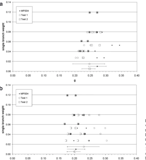
Considering both tests, differences range between -0.084 g and +0.108 g, corresponding to a relative maximum variation of 55% and, generally, the approach of test 1 results in wider differences than the approach of test 2.
3.2. Median maps
The maps shown in Fig. 10 represent MPS04 (median PGA values, Fig. 10a) as well as the differences between such map and the corresponding median PGA map obtained from test 1 (Fig.
71
Fig. 9 - a) Map of the 911 branch in MPS04; b) map of the differences between the 911 branch for MPS04 and the Run 911 for test 1 and c) map of the differences between the 911 branch for MPS04 and the Run 911 for test 2.
a
b
72
Fig. 10 - a) MPS04 median map (MPS Working Group, 2004); b) map of the differences between the MPS04 median map and the test 1 median map and c) map of the differences between the MPS04 median map and the test 2 median map.
a
b
73
10b) and test 2 (Fig. 10c). The same trend, described in the previous section for branch 911, can be observed here too, although we notice that the areas showing large maximum variations are smaller.
Differences between MPS04 and test 1: the map resulting from this approach is strictly dependent on the original b-values. If the original b-value is less than 1, PGA values are smaller than in MPS04 and if the original b-value is larger than 1, PGA values are greater than in MPS04. Again, the maximum variations are in those zones where b-values are most different from 1: minimum negative values are in southern (SSZ 931; original b-values 0.63) and eastern Sicily (SSZ 935, original b-values 0.72 and 0.69); maximum positive values are in north-eastern Italy (SSZ 906, original b-values 1.14 and 1.70) and in northern Apennines (SSZs 913, 914, 915, 919; original b-values 1.44 - 1.80 and 1.23 – 1.70).
Differences between MPS04 and test 2: the map shows a trend similar to the map shown in Fig. 9c and the variations with respect to MPS04 are less evident. The source zones in eastern Sicily (SSZ 935; original values 0.72 and 0.69) and in the Adriatic Sea (SSZ 931; original b-values 0.63) show maximum increased b-values, while only in north-western Italy (SSZs 901, 902, 908, 909; original b-values 1.18 – 1.91 and 1.05 – 1.67) and in the Albani Hills (SSZ 922) do they show negative variations.
The differences between MPS04 and the two tests correspond to a maximum variation of 24% (Fig. 11), limited to small areas with respect to the values in MPS04. However, since in the adopted logic tree the GR branches have a smaller weight than the AR ones (40% vs 60%, Fig. Fig. 11 - Percentage difference maps between MPS04 and test 1 (a) and test 2 (b).
74
1), the impact of a imposed and fixed b-value on SHA is smoothed in the resulting median map.
3.3. Energy release
Another way of assessing the impact of a fixed and an equal to 1 b-value, is considering the energy release: different seismicity rates imply a different amount of released energy.
The energy release for MPS04 and the two tests were evaluated, both for historical and statistical completeness, in 100-year time period, by using the magnitude-energy relation from Gutenberg and Richter (1956):
Log10E(joule) = 4.8 + 1.5 Ms.
For each source zone and for each completeness, we calculated the released energy corresponding to the magnitude of each binned class, and then, we multiplied it for the corresponding rates; the total energy released is the sum of the energy released for all the magnitude classes.
Table 4 shows the energy release for each source zone and for the two different sets of completeness time intervals defined in MPS04; the b-values used in MPS04 are reported too. The comparison between the total energy for the different maps shows that the cumulative energy decreases with respect to MPS04 in both tests and that in test 2 the difference is more significant (9% for test 1 and 20% for test 2). In each source zone the energy release shows a direct correlation with the b-value: it decreases if the b-value is less than 1, whereas it increases if the b-value is greater than 1. Considering the total energy (the sum of the released energy in every source zone), 29 out of 36 SSZs have a b-value greater than 1 (the energy in the tests increases) and 7 out of 36 SSZs have a b-value less than 1 (the energy decreases); the total energy decreases because the contribution of these latest SSZs is more than 50%.
4. Conclusions
In order to investigate new possible options for the logic tree adopted in the MPS04 project (MPS Working Group, 2004), different approaches to the seismicity rate evaluations were explored, according to the current literature, where many theories on the GR distribution are presented.
In the first part of the work, we estimated the b-value variability in the Italian territory: the values obtained confirm a wide variability of this parameter, in agreement with the b-values obtained for the Italian reference hazard map MPS04.
In the second part, we evaluated the impact on the PSHA of using a fixed b-value, through a comparison with MPS04: fixing the b-value to 1, two different approaches, to determine the a-value in the GR distribution, were adopted. The comparison between different approaches was performed at three levels: (1) for a single grid point, (2) for a single logic tree branch and (3) for the median PSHA map. For a single locality a general increase of variability is observed. The analysis of a single logic tree branch highlights differences in PGA values that are greater than in the final map: this is due to the different weights of the logic tree branches that determine a smoothing of the variation in median values with respect to single branch values. Anyway, the
75
differences between MPS04 and the two tests correspond to a maximum variation of 24% . In the final part, setting the b-value to 1 produces a great variation in terms of energy release, that corresponds to a very different distribution in the number of earthquakes per magnitude class compared to the observed one.
In conclusion, the b-value in the Italian territory is extremely variable; this observation, together with the general trend observed in the tests of an increased variability of the final estimates, confirms that the use of a constant and equal to 1 b-value is unrealistic in this area.
Acknowledgement.This research was performed in the frame of the activities of the project S1 (one of the INGV-DPC 2004-06 applied research programs), with the financial support of the Italian Department of Civil Protection (DPC – Dipartimento della Protezione Civile). A special thanks is due to Valentina Montaldo, who encouraged us with valuable and fundamental suggestions from the early steps of the work. The authors would also like to thank two anonymous reviewers for their useful comments which helped to improve the article.
REFERENCES
Ambraseys N.N., Simpson K.A. and Bommer J.J.; 1996: Prediction of horizontal response spectra in Europe. Earth. Eng. Struct. Dyn., 25, 371-400.
Bayrak Y., Yilmazturk A. and Ozturk S.; 2002: Lateral variations of the modal (a/b) values for the different regions of
the world. J. Geodyn., 34, 653-666.
CPTI Working Group; 2004: Catalogo Parametrico dei Terremoti Italiani, versione 2004 (CPTI04). INGV, Bologna, http://emidius.mi.ingv.it/CPTI/.
Gutenberg B. and Richter C.F.; 1944: Frequency of earthquakes in California. Bull. Seismol. Soc. Am., 34, 185-188. Gutenberg B. and Richter C.F.; 1956: Magnitudes and energy of earthquakes. Ann. Geofis., 9, 1-15.
Kagan Y.Y.; 2002: Seismic moment distribution revisited: I. Statistical results. Geophys. J. Int., 148, 520-541. Krinitzsky E.L.; 1993: Earthquake probability in engineering-Part 2: earthquake recurrence and limitations of
Gutenberg-Richter b-values for the engineering of critical structures. Eng. Geol., 36, 1-52.
Lomnitz-Adler J.; 1992: Interplay of fault dynamics and fractal dimension in determining Gutenberg and Richter’s
b-value. Geophys. J. Int., 108, 941-944.
Lopez Casado C., Sanz de Galdano C., Delgado J. and Peinado M.A.; 1995: The b parameter in the Betic Cordillera,
Rif and nearby sectors. Relations with the tectonics of the region. Tectonophysics, 248, 277-292.
Marzocchi W. and Sandri L.; 2003: A review and new insights on the estimation of the b-value and its uncertainty. Ann. Geophys., 46, 1271-1282
McGuire R.K.; 2004: Seismic hazard and risk analysis. EERI, MNO-10, Okland, CA, 221 pp.
Meletti C., Galadini F., Valensise G., Stucchi M., Basili R., Barba S., Vannucci G. and Boschi E.; 2007: The ZS9 seismic
source model for the seismic hazard assessment of the Italian territory. Tectonophysics, submitted.
Montaldo V., Faccioli E., Zonno G., Akinci A. and Malagnini L.; 2005: Treatment of ground-motion predictive
76
MPS Working Group; 2004: Redazione della Mappa di Pericolosità sismica prevista dall’Ordinanza PCM 3274 del 20
marzo 2003. Rapporto conclusivo per il Dipartimento della Protezione Civile, INGV, Milano-Roma, aprile 2004,
65 pp. + 5 appendici, http://zonesismiche.mi.ingv.it/.
Olsson R.; 1999: An estimation of the maximum b-value in the Gutenberg-Richter relation. Geodynamics, 27, 547-552. Oncel A.O., Main I., Alptekin O. and Cowie P.; 1996: Spatial variations of fractal properties of seismicity in the
Anatolian fault zones. Tectonophysics, 257, 189-202.
Pacheco J.F., Scholtz C.H. and Sykes L.R.; 1992: Changes in frequency-size relationship from small to large
earthquakes. Nature, 355, 71-73.
Schorlemmer D. and Wiemer S.; 2005: Microseismicity data forecast rupture area. Nature, 434, 1086.
Schorlemmer D., Wiemer S. and Wyss M.; 2004a: Earthquake statistics at Parkfield: 1. Stationarity of b values. J. Geophys. Res., B12307, doi: 10.1029/2004JB003234.
Schorlemmer D., Wiemer S., Wyss M. and Jackson D.D.; 2004b: Earthquake statistics at Parkfield: 2. probabilistic
forecasting and testing. J. Geophys. Res., B12308, doi: 10.1029/2004JB003235.
Schorlemmer D., Wiemer S. and Wyss M.; 2005: Variations in earthquake-size distribution across different stress
regimes. Nature, 437, 539-542.
Shanker D. and Sharma M.L.; 1998: Estimation of seismic hazard parameters for the Himalayas and its vicinity from
complete data files. Pure appl. geophys., 152 , 267–279.
Wiemer S. and Schorlemmer D.; 2007: ALM: An Asperity-based Likelihood Model for California. Seismol. Res. Letters., 78 (1), 134-140.
Corresponding author: Laura Gulia
Istituto Nazionale di Geofisica e Vulcanologia Via della Faggiola 32, 56126 Pisa, Italy
THE INFLUENCE OF b-VALUE ESTIMATE IN SEISMIC HAZARD ASSESSMENT
Gulia L., Meletti C.
In any probabilistic seismic hazard assessment, an important role is played by the seismicity rates.
This is confirmed by the wide and controversial discussions about the procedures for determination
of them: Gutenberg and Richter distribution or independent rates in every magnitude class, size of
binned magnitude class, least squares or maximum likelihood fit, and so on.
In 2004 a new seismic hazard reference map of Italy (MPS04) has been released adopting a logic
tree approach for exploring the alternative epistemic choices. One of these choices was about the
modality for compute seismicity rates: in the branches where Gutenberg and Richter distribution
(GR) were adopted, the corresponding b-value was evaluated for each source zone, ranging from
0.63 to 2.
These results appeared in contrast with the affirmation of the authors that the b-value is equal to 1
on a worldwide scale and for large volumes; on the other hand many papers pointed out the
spatio-temporal b-value variability related to different parameters, the local stress regime amongst others.
In this work it has been evaluated the effect of the equal to 1 b-value on the results of seismic
hazard assessment. Two different approach have been used: i) the a-value in the GR distribution
derive from MPS04; ii) the a-value has been evaluated in each source zones adopting the least
squares method to fit individual rates. The first case involves a redistribution of earthquakes in the
magnitude classes in comparison with MPS04, while the second one produces a new a-value, that
means a different cumulative number of earthquakes.
The resulting maps have been compared to MPS04, both in terms of expected PGA and of energy
balance. The analysis also shows the effect with respect to the weighted median values, and
pertinent uncertainties, produced by an integrated logic tree.
mappa di pericolosità sismica prevista dall'Ordinanza PCM 3274 e progettazione di ulteriori sviluppi
Task 1 – Completamento delle elaborazioni relative a MPS04
Deliverable D5
Valutazioni sperimentali di amax provenienti da un albero logico più complesso di quello adottato per la redazione di MPS04
a cura di C. Meletti(1), V. Montaldo(2), L. Gulia(1)
(1)
Istituto Nazionale di Geofisica e Vulcanologia, Sezione di Milano-Pavia;
(2)
Istituto Nazionale di Geofisica e Vulcanologia, Sezione di Milano-Pavia; ora Geomatrix Consultants, Inc.
2101 Webster St. 12th floor Oakland, CA 94612, USA
1 diverse. Sono state valutati diversi approcci alla modellazione della sismicità, sia rispetto al modello di zone sorgente, sia rispetto alle modalità di valutare i tassi di sismicità.
Abstract
In the framework of the logic tree approach, we explored new options, epistemically different from the choices made during the elaboration of MPS04.
Different approaches to the modelling of the seismicity were explored, both considering the available seismogenic models vs a no sources model and considering the procedures adopted for the evaluation of seismicity rates (activity rates vs Gutenberg-Richter earthquake distribution).
Questo deliverable non era inizialmente previsto nel progetto S1 ed è stato aggiunto in un secondo momento, anche su indicazione del comitato di revisori internazionali. La descrizione degli obiettivi di questo deliverable è la seguente:
A titolo sperimentale - e per limitate porzioni del territorio - verranno eseguite valutazioni della pericolosità prendendo in considerazione diverse leggi di attenuazione, modelli alternativi di sorgenti sismiche, di Mmax e di valutazione della completezza, con la definizione di un albero logico più complesso di quanto non utilizzato da MPS04, allo scopo di meglio quantificare i contributi delle incertezze aleatorica e epistemica
La figura 1 schematizza in nero la struttura ad albero logico adottata nella realizzazione della mappa di pericolosità sismica di riferimento del territorio nazionale (MPS04; Gruppo di Lavoro MPS, 2004 e http://zoneismiche.mi.ingv.it). Per quanto riguarda il catalogo storico dei terremoti (CPTI04) e il modello di zone sorgente (ZS9) non sono state adottate scelte alternative in quanto quelle eventualmente utilizzabili al tempo non erano da un punto di vista esclusivamente epistemico significativamente diverse. Sono stati invece adottati due set di intervalli di completezza del catalogo, basati su un approccio prevalentemente storico (Co-04.2) e su un approccio prevalentemente statistico (Co-04.4). Sono state adottate due diverse modalità di calcolo dei ratei sismici nelle zone sismogenetiche, vale a dire tassi individuali nelle diverse classi di magnitudo (AR, activity rates) e tassi secondo una distribuzione di tipo Gutenberg-Richter (GR). Infine per quanto riguarda le relazioni di attenuazione del moto del suolo sono stati utilizzati tre diversi set di parametrizzazione basati su dati di base diversi tra loro: ASB96, relazioni da Ambraseys et al. (1996), relazioni di Sabetta e Pugliese (1996), relazioni di tipo regionale sviluppate in ambito INGV da Malagnini e colleghi (Malagnini et al., 2000; Malagnini et al., 2002; Morasca et al., 2002); queste ultime relazioni sono state adottate con due diverse modalità di attribuzione alle diverse zone sorgente. Il dettaglio sulle scelte dell’albero logico adottate in MPS04 sono descritte in Gruppo di Lavoro MPS (2004), la descrizione delle relazioni di attenuazione è contenuta anche in Montaldo et al. (2005).
2 In rosso nella figura 1 sono invece riportate le opzioni che sono state considerate nell’ambito di questo deliverable e analizzate su aree campione o su tutto il territorio nazionale. Le opzioni in rosso con il bordo tratteggiato sono quelle per le quali non sono stati compiuti test, ma che potrebbero rientrare in gioco qualora si voglia procedere alla realizzazione di una nuova mappa di pericolosità sismica.
Passando a descrivere brevemente le possibili scelte alternative, il modello sismogenetico ZS9 può essere affiancato dall’uso delle “aree sismogenetiche” (Seismogenic areas) recentemente definite all’interno del database delle sorgenti sismogenetiche DISS 3.0 (rilasciato nell’ambito del progetto S2, http://www.ingv.it/DISS). Queste aree necessitano anche della definizione di aree di background che consideri la sismicità che non ricade all’interno delle aree sismogenetiche, più strette delle zone sorgente di ZS9. Un’ulteriore alternativa è l’uso del modello cosiddetto smoothed seismicity, come definito da Frankel (1995), che non prevede la definizione di zone sorgente quindi un input di tipo geologico, bensì viene utilizzata la sismicità del catalogo per modellare il processo sismico. Un esempio di uso parallelo dei diversi modelli viene mostrato per l’area campione del Nord-Est d’Italia.
La definizione dei tassi di sismicità può essere arricchita dall’adozione del metodo di fit della massima verosimiglianza (mle), che secondo la letteratura corrente è più indicato del metodo dei minimi quadrati (lsq) in quanto i valori da “fittare” (il numero cumulato di eventi nelle diverse classi di magnitudo) non sono indipendenti tra loro. Un’altra opzione che è stata più volte richiamata nel dibattito scientifico è l’adozione di una distribuzione GR con b=1, come suggerito dagli autori stessi su scala globale (Gutenberg e Richter, 1944). Anche per questa possibile opzione viene mostrata un’applicazione condotta su scala nazionale.
Infine è possibile utilizzare ulteriori modelli di attenuazione del moto del suolo, secondo quanto disponibile nella letteratura recente, quali le relazioni proposte da Ambraseys et al. (2005), da Bragato e Slejko (2005) o ancora da Mercuri et al. (2006).
3 attentamente valutate e opportunamente pesate in una struttura ad albero logico espanso rispetto a quello adottato in MPS04.
Le attività del deliverable, come già brevemente accennato, si sono indirizzate a valutare due dei principali elementi di input nella valutazione della pericolosità sismica, vale a dire il modello di zone sorgente e le modalità di calcolare i tassi di sismicità. Questo rapporto è pertanto diviso in due parti distinte anche perché realizzate dagli autori in modo autonomo e distinto: le possibili opzioni nell’uso di modelli di sorgente sono state studiate in dettaglio da Valentina Montaldo (anche come parte delle attività di ricerca del proprio dottorato di ricerca), le alternative nelle modalità di calcolo dei tassi di sismicità sono state studiate da Laura Gulia e da Carlo Meletti.
4 test sull’uso di diversi modelli di sorgente.
L’area è caratterizzata da un’estrema eterogeneità dell’attività sismica, sia intermini di magnitudo che di frequenza dei terremoti. Inoltre anche la conoscenza sugli aspetti sismologici, geologici e di sismicità storica, nonché le registrazioni sismometriche e accelerometriche variano molti in numero e attendibilità. Due aspetti interessanti ma allo stesso tempo importanti ai fini della definizione della pericolosità dell’area sono: i) le localizzazioni mal definite di 4 terremoti storici con Mw>6; ii) almeno 1 sorgente sismogenetica probabilmente in grado di generare terremoti distruttivi silente negli ultimi 700 anni.
La pericolosità sismica del Nord-Est d’Italia è stata valutata considerando diversi approcci che possono essere classificati in base alla quantità e alla complessità dei dati geologici e sismologici necessari per la loro definizione.
Il modello più semplice che è stato scelto è quello basato sulla distribuzione spaziale della sismicità (Frankel, 1995). Come elementi di input richiede la localizzazione epicentrale, la magnitudo e il tempo origine dei terremoti; possono essere utilizzate anche informazioni geologiche, ma non sono state usate in questo caso. Il processo sismico è modellato secondo un processo di ricorrenza di Poisson, vale a dire che la sismicità è considerata stazionaria nel tempo.
In un approccio probabilistico di tipo convenzionale al calcolo della pericolosità sismica (approccio di Cornell-McGuire) l’informazione geologica viene introdotta con la definizione delle zone sorgente, che consistono in aree all’interno delle quali le caratteristiche tettoniche e sismologiche sono considerate omogenee. Due modelli di zone sorgente sono stati usati nel corso di questo test:
1. il modello di zone sorgente ZS9 (Meletti et al., 2007) usato per la redazione di MPS04 (Gruppo di Lavoro MPS, 2004), definito sulla base di un criterio prevalentemente sismotettonico, integrato con l’informazione sulla sismicità storica e strumentale (fig. 2);
2. le aree sismogenetiche proposte dal database delle sorgenti sismogenetiche DISS 3.0.1 (Diss Working Group, 2005), che sono definite come quelle aree che rappresentano l’inviluppo dei principali sistemi di faglia per i quali non è possibile definire una segmentazione longitudinale, aree nelle quali avvengono i terremoti maggiormente distruttivi (fig. 3).
Nel seguito vengono proposte le immagini relative ai modelli di zone sorgente utilizzati (ZS9 e aree sismogenetiche) e i risultati della stime compiute (Montaldo, 2006) adottando il modello della “smoothed seismicity” (fig. 4) oppure la zonazione ZS9 (fig. 5) oppure ancora le aree sismogenetiche con zone di background (fig. 6). Tutte le stime sono state realizzate utilizzando i diversi periodi di completezza del catalogo, le due modalità di calcolo dei tassi di sismicità e le diverse relazioni di attenuazione. In particolare la stima ottenuta con l’approccio a “smoothed seismicity” (fig. 4) è la mediana di 6 rami di un albero logico che considera 2 completezze del catalogo (storica e statistica) e 3 relazioni di attenuazione (Ambraseys et al., 1996; Sabetta e Pugliese, 1996; relazioni regionali di Malagnini e colleghi); le mappe ottenute usando i modelli di zona sorgente sono la mediana di 12 uscite di un albero logico che considera 2 completezze del catalogo (storica e statistica), 2 modalità di calcolo dei tassi di sismicità (AR e GR, come in Gruppo di Lavoro , 2004) e 3 relazioni di attenuazione (Ambraseys et al., 1996; Sabetta e Pugliese, 1996; relazioni regionali di Malagnini e colleghi).
5 Figura 3. Aree sismogenetiche definite dal database DISS 3 (release di luglio 2006), confrontate con le sorgenti sismogenetiche individuali e con la sismicità del catalogo CPTI04. Le aree con bordo blu (BKG in legenda) sono le aree di background definite per considerare nel calcolo la sismicità che non ricade dentro le aree sismogenetiche.
6 Figura 5. Stima di pericolosità sismica (probabilità di eccedenza del 10% in 50 anni) utilizzando il modello di zone sorgente ZS9 (Meletti et al., 2007).
Figura 6. Stima di pericolosità sismica (probabilità di eccedenza del 10% in 50 anni) utilizzando il modello di aree sismogenetiche (da DISS 3.0) associate a zone di background.
7 terremoti per l’intervallo temporale (activity rates) e tassi calcolati attraverso la relazione di Gutenberg e Richter (1944). Questa seconda alternativa impiega un diverso b-value per ogni zona della zonazione sismogenetica adottata (ZS9; Meletti et al., 2007).
La presunta variabilità del b-value e la stima a scale differenti di questo parametro sono oggetto, negli ultimi anni, di numerose pubblicazioni. Le principali teorie sono due:
• un valore costante e uguale a 1, non dipendente dalla scala adottata (Kagan,
2002): il processo di generazione dei terremoti sarebbe non solo self-similare ma anche invariante a scala mondiale;
• un b-value variabile (e.g. Schorlemmer et al., 2005; Schorlemmer and
Wiemer, 2005; Wiemer and Schorlemmer, 2007; Shanker and Sharma, 1998; Lomnitz-Adler, 1992; Pacheco et al., 1992) in relazione al differente regime tettonico, a cambiamenti di stress e all’eterogeneità del materiale. In questo studio si è voluto valutare l’impatto dell’adozione di un b-value uguale a 1 sulle stime di hazard attraverso l’elaborazione di una nuova mappa di pericolosità, realizzata utilizzando lo stesso albero logico (Fig. 7)e le stesse soluzioni adottate in MPS04 (Gruppo di Lavoro MPS, 2004), e sostituendo i tassi calcolati con un b-value variabile in ogni ZS dalla relazione di Gutenberg e Richter (1944; d’ora in avanti GR) con i tassi ricalcolati fissando il valore del parametro a 1 (Gulia e Meletti, 2007) in tutte le zone del modello di zonazione sismogenetica ZS9 (Meletti et al., 2007).
Uno degli elementi dell’albero logico per i quali esistono opzioni epistemicamente alternative è la modalità di calcolo dei tassi. Nella redazione di MPS04 sono state adottate due differenti metodologie: calcolo degli activity rates per ogni classe di magnitudo e l’utilizzo della GR. Nell’analisi eseguita, dopo aver fissato il b-value, è stato calcolato il valore del secondo parametro della relazione, il parametro a, secondo due differenti modalità alternative:
x lo stesso a-value adottato in MPS04, cioè lo stesso numero di eventi, test 1;
x un nuovo valore ottenuto attraverso il metodo dei minimi quadrati, test 2.
Come per MPS04, quando la magnitudo massima assunta in ogni ZS è maggiore di quella riportata dal catalogo, i tassi per quella classe di magnitudo sono stati determinati per estrapolazione dalla retta GR determinata.
8 come valutata in MPS04, la distribuzione GR relativa al test 1 e quella relativa al test 2) applicate ai tassi osservati, in due zone sismogenetiche, dove il b-value originale è, rispettivamente, maggiore di 1 (SSZ 915) e minore di 1 (SSZ 935).
SSZ 915 (Fig. 8a): il test 1 ha lo stesso numero totale di eventi di MPS04, ma una
distribuzione differente tra le classi di magnitudo: aumenta il numero dei grandi terremoti e diminuisce quello dei piccoli. Per il test 2 il valore di a è inferiore rispetto a quello di MPS04: ne consegue che il numero di eventi nella zona diminuisce. In conclusione, i tassi di sismicità relativi al test 2 sono inferiori a quelli relativi a MPS04.
SSZ 935 (Fig. 8b): nel test 1 decresce il numero di grandi terremoti rispetto ad
MPS04 e cresce quello relativo ai piccoli. L’ a-value prodotto dal test 2 è maggiore rispetto ad MPS04, decresce il numero di grandi terremoti e aumenta il numero dei piccoli.
Figura 8. a) Distribuzione magnitudo-frequenza in MPS04 –cerchi per i tassi da GR e rombi per gli activity rates- e nei due test –triangoli per il test 1 e quadrati per il test 2.
a) zona sismogenetica con un b-value originale >1 (SSZ 915);
b) zona sismogenetica con un b-value originale <1 (SSZ 935).
Di seguito vengono riportate le distribuzioni magnitudo-frequenza relative alle singole zone sismogenetiche, secondo i due set di intervalli di completezza adottati in MPS04: storico (Fig. 9) e statistico (Fig. 10).
Figura 9a. Tassi di si
smicità nelle zone sorgente
da 901 a
9
09 in base
all’
adozione della comp
letezza storica del catalogo e al
le diverse modalità
di calco
Figura 9b.
Tassi di sismicità ne
lle zone sorgente
da 910 a
9
18 in base
all’adoz
ione della comp
letezza storica del catalogo e al
le d
iverse modalità
di calco
Figura 9c.
Tassi di sismicità ne
lle zone sorgente
da 919 a
9
27 in base
all’adoz
ione della comp
letezza storica del catalogo e al
le d
iverse modalità
di calco
Figura 9d.
Tassi di sismicità ne
lle zone sorgente
da 928 a
9
36 in base
all’adoz
ione della comp
letezza storica del catalogo e al
le diverse modalità
di calco
Figura 10a. Tassi di sismic ità nelle zone sorgente da 901 a 909 in base all’ad ozion
e della completezza sta
tistica del catalogo
e alle diverse
modalità di calcolo utiliz
Figura 10b. Tassi di sismicità ne lle zone sorgente da 910 a 918 in base all’adozio n e
della completezza sta
tistica del catalogo
e alle diverse
modalità di calcolo utiliz
Figura 10c. Tassi di sismicità ne lle zone sorgente da 919 a 927 in base all’adozio n e
della completezza sta
tistica del catalogo
e alle diverse
modalità di calcolo utiliz
Figura 10d. Tassi di sismicità ne lle zone sorgente da 928 a 936 in base all’adozio n e
della completezza sta
tistica del catalogo
e alle diverse
modalità di calcolo utiliz
17 Impatto su un singolo ramo dell’albero logico
L’analisi di un singolo ramo è stata effettuata attraverso il confronto tra le mappe ottenute secondo le scelte del ramo 911 in MPS04 (Gruppo di Lavoro MPS, 2004) e nei due test (Gulia e Meletti, 2007), vale a dire: completezza storica, tassi da GR e relazione di attenuazione del moto del suolo secondo Ambraseys et al. (1996).
In figura 11a è riportata la mappa ottenuta in MPS04 per il ramo 911, mentre le figure 11b e 11c riportano, rispettivamente, la mappa delle differenze tra MPS04 e il test 1 e tra MPS04 e il test 2. Nelle aree azzurre i valori di PGA in MPS04 sono inferiori rispetto ai test e in quelle rosse sono maggiori. In particolare:
x per il test 1 le differenze negative sono localizzate nelle zone sismogenetiche
dell’Appennino settentrionale (SSZ 913, 914, 915, 919, 921) e nell’area Eolie-Patti (SSZ 932), nella quali i b-value “originali” sono maggiori di 1.22; differenze positive si osservano invece nel sud Italia (SSZ 925, 929, 931) e nella Sicilia orientale (SSZ 935), dove il b-value valutato in MPS04 è minore di 0.82; le differenze più marcate si osservano nelle zone sismogenetiche che in MPS04 hanno un b-value molto diverso da 1;
x per il test 2 si hanno differenze meno marcate rispetto al caso precedente. Le
differenze positive maggiori sono nelle zone 925 (Ofanto; b-value in MPS04 di 0.67) e 931 (Canale d’Otranto; b-value in MPS04 di 0.63); le differenze negative maggiore sono nella zona 901 (Savoia; b-value in MPS04 di 1.18) e 927 (Irpinia-Basilicata; b-value in MPS04 di 0.71). In generale nel test 2 non si osservano chiare relazioni tra il valore di b valutato in MPS04 e le variazioni della stima dell’hazard; differenze significative, infatti, si osservano anche in zone con un b-value originale non molto dissimile da 1, come nel nord-est (1.06), nell’Appennino centrale (1.05) e nella Sicilia occidentale (0.96).
In entrambi i test le differenze raggiungono un valore massimo di circa il 24% e, generalmente, il test 1 produce variazioni maggiori che non il test 2.
a b c Figura 11. a) Mappa r e lat iva al ra mo 911 in MPS04 ; b)
differenze tra il ramo 911 in MPS0
4 e il ramo
911 nel
test 1
; c) diffe
renze tra il ramo
911 in MPS
04 e il ramo 911 nel
tes
t 2