2020-06-29T09:59:06Z
Acceptance in OA@INAF
The ALMA Spectroscopic Survey in the Hubble Ultra Deep Field: Molecular Gas
Reservoirs in High-redshift Galaxies
Title
DECARLI, ROBERTO; Walter, Fabian; Aravena, Manuel; Carilli, Chris; Bouwens,
Rychard; et al.
Authors
10.3847/1538-4357/833/1/70
DOI
http://hdl.handle.net/20.500.12386/26262
Handle
THE ASTROPHYSICAL JOURNAL
Journal
833
THE ALMA SPECTROSCOPIC SURVEY IN THE HUBBLE ULTRA DEEP FIELD: MOLECULAR GAS
RESERVOIRS IN HIGH-REDSHIFT GALAXIES
Roberto Decarli1, Fabian Walter1,2,3, Manuel Aravena4, Chris Carilli3,5, Rychard Bouwens6, Elisabete da Cunha7,8, Emanuele Daddi9, David Elbaz9, Dominik Riechers10, Ian Smail11, Mark Swinbank11, Axel Weiss12, Roland Bacon13,
Franz Bauer14,15,16, Eric F. Bell17, Frank Bertoldi18, Scott Chapman19, Luis Colina20, Paulo C. Cortes21,22, Pierre Cox21, Jorge GÓnzalez-LÓpez23, Hanae Inami13, Rob Ivison24,25, Jacqueline Hodge6, Alex Karim18,
Benjamin Magnelli18, Kazuaki Ota5,26, Gergö Popping24, Hans-Walter Rix1, Mark Sargent27, Arjen van der Wel1, and Paul van der Werf6
1
Max-Planck Institut für Astronomie, Königstuhl 17, D-69117, Heidelberg, Germany;[email protected]
2
Astronomy Department, California Institute of Technology, MC105-24, Pasadena, CA 91125, USA
3
National Radio Astronomy Observatory, Pete V. Domenici Array Science Center, P.O. Box O, Socorro, NM 87801, USA
4
Núcleo de Astronomía, Facultad de Ingeniería, Universidad Diego Portales, Av. Ejército 441, Santiago, Chile
5
Cavendish Laboratory, University of Cambridge, 19 J J Thomson Avenue, Cambridge CB3 0HE, UK
6
Leiden Observatory, Leiden University, P.O. Box 9513, NL2300 RA Leiden, The Netherlands
7
Centre for Astrophysics and Supercomputing, Swinburne University of Technology, Hawthorn, Victoria 3122, Australia
8
Research School of Astronomy and Astrophysics, Australian National University, Canberra, ACT 2611, Australia
9
Laboratoire AIM, CEA/DSM-CNRS-Universite Paris Diderot, Irfu/Service d’Astrophysique, CEA Saclay, Orme des Merisiers, F-91191 Gif-sur-Yvette cedex, France
10
Cornell University, 220 Space Sciences Building, Ithaca, NY 14853, USA
11
6 Centre for Extragalactic Astronomy, Department of Physics, Durham University, South Road, Durham, DH1 3LE, UK
12
Max-Planck-Institut für Radioastronomie, Auf dem Hügel 69, D-53121 Bonn, Germany
13
Université Lyon 1, 9 Avenue Charles André, F-69561 Saint Genis Laval, France
14
Instituto de Astrofísica, Facultad de Física, Pontificia Universidad Católica de Chile Av. Vicuña Mackenna 4860, 782-0436 Macul, Santiago, Chile
15
Millennium Institute of Astrophysics(MAS), Nuncio Monseñor Sótero Sanz 100, Providencia, Santiago, Chile
16
Space Science Institute, 4750 Walnut Street, Suite 205, Boulder, CO 80301, USA
17
Department of Astronomy, University of Michigan, 1085 South University Avenue, Ann Arbor, MI 48109, USA
18Argelander Institute for Astronomy, University of Bonn, Auf dem Hügel 71, D-53121 Bonn, Germany 19
Dalhousie University, Halifax, Nova Scotia, Canada
20
ASTRO-UAM, UAM, Unidad Asociada CSIC, Spain
21
Joint ALMA Observatory—ESO, Av. Alonso de Córdova, 3104, Santiago, Chile
22
National Radio Astronomy Observatory, 520 Edgemont Road, Charlottesville, VA 22903, USA
23
Instituto de Astrofísica, Facultad de Física, Pontificia Universidad Católica de Chile Av. Vicuña Mackenna 4860, 782-0436 Macul, Santiago, Chile
24
European Southern Observatory, Karl-Schwarzschild-Strasse 2, D-85748, Garching, Germany
25
Institute for Astronomy, University of Edinburgh, Royal Observatory, Blackford Hill, Edinburgh EH9 3HJ, UK
26
Kavli Institute for Cosmology, University of Cambridge, Madingley Road, Cambridge CB3 0HA, UK
27
Astronomy Centre, Department of Physics and Astronomy, University of Sussex, Brighton, BN1 9QH, UK Received 2016 May 3; revised 2016 September 5; accepted 2016 September 6; published 2016 December 8
ABSTRACT
We study the molecular gas properties of high-z galaxies observed in the ALMA Spectroscopic Survey(ASPECS) that targets an∼1 arcmin2region in the Hubble Ultra Deep Field(UDF), a blind survey of CO emission (tracing molecular gas) in the 3 and 1 mm bands. Of a total of 1302 galaxies in the field, 56 have spectroscopic redshifts and correspondingly well-defined physical properties. Among these, 11 have infrared luminositiesLIR>1011L, i.e.,
a detection in CO emission was expected. Out of these, 7 are detected at various significance in CO, and 4 are undetected in CO emission. In the CO-detected sources, wefind CO excitation conditions that are lower than those typically found in starburst/sub-mm galaxy/QSO environments. We use the CO luminosities (including limits for non-detections) to derive molecular gas masses. We discuss our findings in the context of previous molecular gas observations at high redshift(star formation law, gas depletion times, gas fractions): the CO-detected galaxies in the UDF tend to reside on the low-LIR envelope of the scatter in theLIR–LCO¢ relation, but exceptions exist. For the
CO-detected sources, wefind an average depletion time of ∼1 Gyr, with significant scatter. The average molecular-to-stellar mass ratio (MH2/M*) is consistent with earlier measurements of main-sequence galaxies at these
redshifts, and again shows large variations among sources. In some cases, we also measure dust continuum emission. On average, the dust-based estimates of the molecular gas are a factor∼2–5× smaller than those based on CO. When we account for detections as well as non-detections, wefind large diversity in the molecular gas properties of the high-redshift galaxies covered by ASPECS.
Key words: galaxies: evolution– galaxies: ISM – galaxies: star formation – galaxies: statistics – instrumentation: interferometers– submillimeter: galaxies
1. INTRODUCTION
Molecular gas observations of galaxies throughout cosmic time are fundamental for understanding the cosmic history of the formation and evolution of galaxies (see reviews by
Kennicutt & Evans 2012; Carilli & Walter 2013). The molecular gas provides the fuel for star formation, thus by characterizing its properties we place quantitative constraints
on the physical processes that lead to the stellar mass growth of galaxies. This has been a demanding task in terms of telescope time. To date, only some several hundred sources atz>1 have been detected in a molecular gas tracer(typically the rotational transitions of the carbon monoxide 12CO molecule; e.g., Carilli & Walter2013). This sample is dominated by “extreme” sources, such as QSO host galaxies(e.g., Bertoldi et al.2003; Walter et al. 2003; Weiß et al. 2007; Wang et al. 2013) or submillimeter galaxies (e.g., Frayer et al. 1998; Neri et al. 2003; Greve et al.2005; Bothwell et al.2013; Riechers et al. 2013; Aravena et al. 2016), with IR luminosities
LIR 1012 L and star formation rates (SFRs) 100
M yr−1. These extreme sources might contribute significantly to the star formation budget in the universe atz>4, but their role declines with cosmic time(Casey et al.2014). Indeed, the bulk of star formation up toz~2 is observed in galaxies along the so-called“main sequence” (Elbaz et al.2007,2011; Noeske et al. 2007; Daddi et al. 2010a, 2010b; Genzel et al. 2010; Wuyts et al. 2011; Whitaker et al.2012), a tight (scatter rms ∼0.3 dex) relation between the SFR and the stellar mass, M*. Addressing the molecular gas content of main-sequence galaxies beyond the local universe has become feasible only in recent years.
The first step in the characterization of the molecular gas content of galaxies is the measure of the molecular gas mass,
MH2. The 12CO molecule (hereafter, CO) is the second most
abundant molecule in the universe, and it is relatively easy to target thanks to its bright rotational transitions. The use of CO as a tracer for the molecular gas mass requires assuming a conversion factor, aCO, to pass from CO(1–0) luminosities to
H2masses. Atz~0, the conversion factor that is typically used
is ∼4M(Kkm s−1pc2)−1 for “normal” * >M 109 M
star-forming galaxies with metallicities close to solar (see Bolatto et al. 2013, for a recent review). If other CO transitions are observed instead of the J=1 0 ground state transition, a further factor is required to account for the CO excitation(see, e.g., Weiß et al. 2007; Daddi et al.2015). Tacconi et al. (2010) and Daddi et al.(2010a) investigated the molecular gas content of highly star-forming galaxies at z~1.2 and z~2.3 via the CO(3–2) transition. They found large reservoirs of gas, yielding molecular-to-stellar mass ratios MH2 M* ~ 1. These values are significantly higher than those observed in local galaxies (∼0.1, see, e.g., Leroy et al. 2008), suggesting a strong evolution of
*
MH2 M with redshift (see also Riechers et al. 2010; Casey
et al. 2011; Geach et al. 2011; Aravena et al. 2012, 2016; Magnelli et al.2012; Bothwell et al.2013; Saintonge et al.2013; Tacconi et al.2013; Chapman et al.2015a; Genzel et al.2015). An alternative approach to estimate gas masses is via dust emission. The dust mass in a galaxy can be retrieved via the study of its rest-frame submillimeter spectral energy distribu-tion (SED) (e.g., Magdis et al. 2011, 2012; Magnelli et al. 2012; Santini et al. 2014; Béthermin et al.2015; Berta et al.2016), in particular via the Rayleigh–Jeans tail, which is less sensitive to the dust temperature (see, e.g., Scoville et al.2014; Groves et al.2015). Using the dust as a proxy of the molecular gas does not require assumptions on CO excitation and on aCO. However, this approach relies on the assumption
of a dust-to-gas mass ratio(DGR), which typically depends on the gas metallicity(Bolatto et al.2013; Sandstrom et al.2013; Genzel et al. 2015). Recent ALMA results report substantially lower values of Mgas than what are typically obtained in
CO-based studies(Scoville et al.2014,2016).
In the present paper, we study the molecular gas properties of galaxies in ASPECS, the ALMA Spectroscopic Survey in the Hubble Ultra Deep Field(UDF). This is a blind search for CO emission using the Atacama Large Millimeter /submilli-meter Array (ALMA). The goal is to constrain the molecular gas content of an unbiased sample of galaxies. The targeted region is one of the best-studied areas of the sky, with exquisitely deep photometry in >25 X-ray-to-far-infrared(IR) bands, photometric redshifts, and dozens of spectroscopic redshifts. This provides us with an exquisite wealth of ancillary data, which is instrumental to place our CO measurements in the context of galaxy properties. Thanks to the deep-field nature of our approach, we avoid potential biases related to the preselection of targets, and include both detections and non-detections in our analysis. Our data set combines 3 mm and 1 mm observations of the same galaxies, thus providing constraints on the CO excitation. Furthermore, the combination of the spectral line survey and the 1 mm continuum image allows us to compare CO- and dust-based estimates of the gas mass. In other papers of this series, we present the data set and the catalog of blindly selected CO emitters (Paper I, Walter et al.2016), we study the properties of 1.2 mm detected sources (Paper II, Aravena et al. 2016a), we discuss the inferred constraints on the luminosity functions of CO (Paper III, Decarli et al. 2016a), and we search for [CII] emission in z=6–8 galaxies (Paper V, Aravena et al. 2016b). Paper VI (Bouwens et al.2016) places our findings in the context of the dust extinction law forz>2 galaxies, and Paper VII (Carilli et al. 2016) uses ASPECS to place first direct constraints on intensity mapping experiments. Here we place the CO detections in the context of the properties of the associated galaxies. In Section2we summarize the observational data set; in Section3 we describe our sample; in Section 4we present CO-based measurements, which are discussed in the context of galaxy properties in Section5. We summarize our findings in Section6.
Throughout the paper we assume a standard ΛCDM cosmology with H0=70 km s−1 Mpc−1, Wm = 0.3, and
W =L 0.7(broadly consistent with the measurements in Planck Collaboration XIII2016), and a Chabrier (2003) initial stellar mass function. Magnitudes are expressed in the AB photo-metric system(Oke & Gunn 1983).
2. OBSERVATIONS 2.1. The ALMA Data Set
The details of the ALMA data set (observations and data reduction) are presented in PaperI of this series. Here we briefly summarize the observational details that are relevant for the present study. The data set consists of two frequency scans in ALMA band 3(3 mm, 84–115 GHz) and in band 6 (1 mm, 212–272 GHz). In the case of the 3 mm observations, we obtained a single pointing centered at R.A.=03:32:37.900, decl.=–27:46:25.00 (J2000.0), close to the northern corner of the Hubble eXtremely Deep Field (XDF, Illingworth et al.2013). The primary beam has a diameter of » 65 at the central frequency of the band (99.5 GHz). The typical noise rms is ∼0.18 mJy beam−1 per 50 km s−1 channel. The 1 mm observations consist of a seven-pointing mosaic covering approximately the same area as the 3 mm observations. The typical noise rms is 0.44 mJy beam−1 per 50 km s−1 channel.
The resulting 1 mm continuum image reaches a noise rms of 12.7μJy beam−1at the center of the mosaic(see PaperII).
2.2. Ancillary Data
We complement the ALMA data with X-ray-to-far-IR photometry from public catalogs of this field, as well as optical/near-IR spectroscopic information where available. The main sources for the photometry are the compilations by Coe et al. (2006) and Skelton et al. (2014). The former includes optical photometry based on the original Hubble Space Telescope (HST) Advanced Camera for Survey (ACS) images of the Hubble UDF(Beckwith et al.2006) and near-IR images obtained with HST NICMOS. The latter also compiles optical/ near-IR observations with HST ACS and the Wide Field Camera 3 (WFC3) from the Hubble XDF (Illingworth et al. 2013), Spitzer IRAC, as well as a wealth of ground-based optical /near-IR observations. Spitzer MIPS data at 24 and 70μm, as well as Herschel PACS and SPIRE data come from the work by Elbaz et al. (2011). X-ray data are taken from the Extended Chandra Deep Field South Survey (Lehmer et al. 2005) and from the Chandra Source Catalog (Evans et al.2010).
Photometric redshifts (zphoto) are available for all of the
optically selected sources in thefield. At a limiting magnitude i=28 mag, the median uncertainty is dzphoto~0.5, and it reaches dzphoto~1 at i»30 mag (Coe et al. 2006). The compilation of Skelton et al.(2014) provides even more robust photometric redshifts, thanks to the expanded photometric data set. The agreement with available spectroscopic redshifts is typically very good in these cases, with a standard deviation on Dz (1 +z) of »0.01(Skelton et al.2014). In addition, the 3D-HST survey provides 3D-HST ACS and WFC3 grism observations of the field, yielding grism redshifts for tens of sources in our pointing (Momcheva et al. 2016). Slit spectroscopy for 74 (mostly bright) galaxies in the field is also available (Le Fèvre et al. 2005; Skelton et al. 2014; Morris et al.2015). Finally, integral field spectroscopy of this field has been secured with the ESO Very Large Telescope/MUSE. These data are part of a Guaranteed Time observing program targeting the UDF. In particular, a single(1 arcmin2) deep (21 hr on source) pointing overlaps with∼70% of the ASPECS coverage. The cubes have been processed and analyzed with the improved MUSE GTO pipeline. These observations will be presented in R. Bacon et al.(2016, in preparation).
Within a radius of34 from the ALMA 3 mm pointing center (approximately the size of the primary beam of our 3 mm observations), there are 1302 galaxies from the combination of all the available photometric catalogs. We use the high-z extension of MAGPHYS(da Cunha et al.2008,2015) to fit the SEDs of all of them. The input photometry includes 26 broad and medium filters ranging from observed U band to Spitzer IRAC 8μm. Additionally, we include the ASPECS 1 mm continuum photometry for those sources where >2-σ emission is reported in our 1 mm continuum image. We do not include any Spitzer MIPS or Herschel PACS photometry because the angular resolutions of these instruments are not sufficient to accurately pinpoint the emission.28 Our MAGPHYS analysis
provides us with a posterior probability distribution of the stellar mass ( *M ), the SFR, the specific SFR (sSFR=SFR/
*
M ), the dust mass (Mdust), and the IR luminosity for each
galaxy in thefield. We take the 14% and 86% quartiles of the posterior distributions as the uncertainties in the parameters, and we account for an additionalfiducial 10% uncertainty that is due to systematics (subtleties in the photometric analysis adopted in the input catalogs, such as aperture corrections and deblending assumptions; zero-point uncertainties; etc.). Figure1 shows the SFR as a function of M*for all the 1302 galaxies in ourfield.
3. THE SAMPLE
We focus our discussion on those galaxies in the field covered by ASPECS that we originally expected to detect in CO emission. Our expectations are based on the MAGPHYS predictions discussed in the previous section. Figure1 shows the stellar masses and SFRs of all 1302 galaxies in the field (color–coded by redshift). Out of these, 56 galaxies have secure spectroscopic redshifts within our CO redshift coverage, and are brighter than 27.5 mag in thefilters F850LW or F105W (z and Y bands, respectively).29We further restrict our analysis to the redshift windows for which ASPECS covers at least one of Figure 1. Star formation rates and stellar masses of all the galaxies in our field, color-coded by redshift. Inferred parameters are derived using the high-z extension of MAGPHYS(da Cunha et al.2008,2015). The sample discussed here is highlighted with large symbols: diamonds refer to the CO detections, while galaxies in the present sample that are not detected in CO are marked with triangles. We stress that only galaxies with secure spectroscopic redshifts are considered in the present analysis. The loci of the main sequence in various redshift bins are shown as dotted lines(from Whitaker et al.2012) and dashed lines(from Schreiber et al.2015). Half of the galaxies in our sample lie along the main sequence at their respective redshifts. ID.5, 7, and 11 occupy the “starburst” region above the main sequence, while ID.3 and 6 exhibit an SFR ~ ´3 lower than what is typically observed in main-sequence galaxies at the same redshifts and stellar masses.
28
For instance, including MIPS and PACS in the SED fits yields an overestimate(by a factor ∼3) of the SFR in the brightest source in our sample, but with a poor SEDfit quality, because of the contamination of foreground sources; on the other hand, the second brightest galaxy, which appears isolated, shows consistent results regardless of whether the fit is performed with or without MIPS and PACS photometry.
29
Thisflux cut allows us to reject sources that are too faint for a reliable SED analysis.
the following low-J CO transitions: J=2 1,J=32, or J=43.
From these galaxies, we select the 11 galaxies for which the MAGPHYS SED analysis yields an IR luminosity LIR >1011
L at >1σ significance. These sources are marked by symbols in Figure1, and spectroscopic redshifts are available for all of these sources. The IR luminosity of a galaxy(derived from the SED
fitting) has been found to correlate with the CO luminosity (see also Section5.2.1). Following the best fit of the relation in Carilli & Walter (2013), the IR-luminosity cut above corresponds to
¢ - > ´
LCO 1 0( ) 3 109 Kkm s−1pc
2
, i.e., it is similar to the line luminosity limit of our survey(see PaperI). Consequently, we should be able to detect CO, or at least place meaningful limits, on these 11 galaxies.
Table 1
Sample of Galaxies Examined in this Work, and Their Optical/near-IR Global Properties
ID ASPECS Optical R.A. Optical decl. z Obs.CO M* SFR sSFR LIR Re
Name Trans. (´109 M ) (M yr −1) (Gyr−1) (´1011L) (kpc) (1) (2) (3) (4) (5) (6) (7) (8) (9) (10) (11) 1 3 mm.1a, C1 03:32:38.54 −27:46:34.0 2.543 3, 7, 8 17.8-+1.71.8 63+-66 3.4-+0.310.34 12.3-+1.11.2 1.7 2 3 mm.2, C2 03:32:39.74 −27:46:11.2 1.551 2, 5, 6 275-+4070 74-+3060 0.27-+0.140.27 12.0-+4.38.6 8.3 3 3 mm.3 03:32:35.55 −27:46:25.5 1.382 2, 5 52-+1012 18+-79 0.42-+0.250.13 1.9-+0.91.3 8.3 4 3 mm.5, C6 03:32:35.48 −27:46:26.5 1.088 2, 4 28-+57 23-+920 0.9-+0.40.9 2.8-+1.22.4 5.8 5 L 03:32:36.43 −27:46:31.8 1.098 2, 4 5.8-+0.50.6 44+-44 7.41-+0.70.7 15.5-+1.41.5 6.0 6 C7 03:32:35.78 −27:46:27.5 1.094 2, 4 75-+1312 16+-611 0.21-+0.080.17 3.1-+1.11.5 3.8 7 L 03:32:39.08 −27:46:01.8 1.221 2, 5 15.1-+1.41.5 148+-1315 9.3-+0.80.9 49.0-+4.44.9 0.7 8 03:32:36.66 −27:46:31.0 0.999 4 70-+1711 40-+914 0.54-+0.050.40 7.1-+2.51.5 6.6 9 L 03:32:39.41 −27:46:22.4 2.447 3, 7, 8 2.6-+0.20.3 11.8-+1.11.2 4.2-+0.40.4 1.35-+0.120.13 5.8 10 L 03:32:37.07 −27:46:17.2 2.224 3, 6, 7 12.0-+1.21.2 22+-241 1.86-+0.173.53 1.95-+0.185.3 2.7 11 L 03:32:36.33 −27:46:00.1 0.895 4 15.9-+1.49.0 42+-124 2.7-+1.50.27 5.8-+1.60.6 1.2
Notes.Sorting is based on the significance of the CO detection. (1) Source ID. (2) ASPECS name for blind CO detections (3 mm.X, see PaperI) and for the blind 1.2 mm continuum detections(CX, see PaperII). (3)–(4) Optical coordinates in Skelton et al. (2014). (5) Redshift. (6) Jupof the CO transitions encompassed in our
ASPECS Data.(7)–(10) MAGPHYS-derived stellar mass (M*), star formation rate (SFR), specific star formation rate (sSFR), IR luminosity (LIR). (11) Effective
radius from the near-IR analysis by van der Wel et al.(2012).
a
Also 1 mm.1 and 1 mm.2, see PaperI.
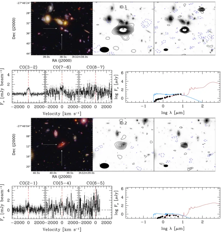
Figure 2. Top left: HST F105W/F775W/F435W RGB image of ID.1. The postage stamp is ´20 20 . Top center: HST F125W image of the same field. The map of the lowest-J accessible CO transition(in this case, CO[3–2]) is shown as contours (2, 3,¼, 20‐s[σ(ID.1)=0.78 mJy beam−1]; solid black lines for the positive isophotes, dashed blue lines for the negative). The synthesized beam is shown as a black ellipse. Top right: same as in the center, showing the 1.2 mm dust continuum. Bottom left: spectra of the CO lines encompassed in our spectral scan. Bottom right: spectral energy distribution. The red line shows the best MAGPHYSfit of the available photometry(black points), while the blue line shows the corresponding model for the unobscured stellar component. The main output parameters are quoted. Similar plots for all the sources in our sample are available in this paper.
Table1 summarizes the main optical/near-IR properties of the galaxies considered in this paper. In Figure2 we show for one of the sources the HST image compared with the CO and dust continuum maps, the CO spectra, and the SED data and modeling. Similar plots are presented for all sample galaxies in this paper.
Four of the galaxies in our sample match some of the CO lines identified in our blind search (see PaperI). The ASPECS name for these sources is also reported in Table 1. Three additional galaxies show CO emission, although at lower significance. Finally, four sources remain undetected in CO.
3.1. Notes on Individual Galaxies
ID.1 (Table 1, Figures 2 and 11) is a compact galaxy at »
z 2.5. Momcheva et al. (2016) report a grism redshift z=2.561, based on the detection of the [OII] line in the 3D-HST data. This redshift is improved by our blind detection of three CO transitions (ASPECS 3 mm.1, 1 mm.1, 1 mm.2; see PaperI), clearly pininng down the redshift to z=2.543. The HST images show a blue component in the north and a red component in the south (or possibly a single relatively blue component that is partially reddened in the south by a thick dust lane). A group of bright galaxies is present a few arcsec north of this galaxy, but their spectroscopic redshifts show that the group is in the foreground, with only one other source lying at z~2.5 (the galaxy ~ 2 west of ID.1). The starlight emission coincident with the CO detection is compact, with a scale radiusRe»1.7 kpc (van der Wel et al.2012). Chandra reveals X-ray emission associated with this galaxy. The measured X-ray flux is FX=5.7´10-17 erg s−1cm−2,
yielding an X-ray luminosity LX=3.0´1042 erg s−1 (Xue et al.2011).
ID.2(Figure11) has an HST morphology consistent with a large disk galaxy at z=1.552. Its slit redshift (z=1.552, Kurk et al.2013) matches our CO line detection well (ASPECS 3 mm.2), assuming CO(2–1). The disk has an inclination of ~60(based on the aspect ratio, van der Wel et al. 2012), with an effective radius of 8.3 kpc. The galaxy is detected with Chandra. Xue et al. (2011) report a flux of
= ´
-FX 3.6 10 15erg s−1cm−2(but2.6´10-15erg s−1cm−2 in Lehmer et al. 2005), yielding an X-ray luminosity
= ´
LX 5.5 1043erg s−1, suggesting that ID.2 hosts an active galactic nucleus(AGN).
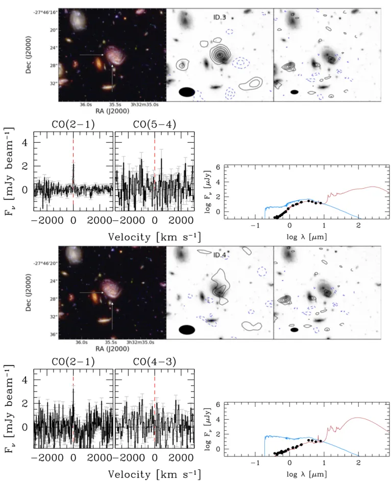
ID.3 and ID.4 (Figure 12) are the two components of an apparent pair of overlapping spiral galaxies. The southern component exibits bright [OII] emission at ∼7784 Å (see Figure3), clearly placing it at z=1.088 (in agreement with the CO redshift of ASPECS 3 mm.5); the northern component shows bright CO emission(ASPECS 3 mm.3), which could be interpreted as CO(2–1) at z=1.382. Our careful analysis of the MUSE data around 8880Å reveals faint [OII] emission (although contaminated by sky line emission), supporting the CO identification (see Figure 3). The disk of ID.4 has a scale radius of 5.8 kpc based on HST imaging (van der Wel et al. 2012); for ID.3, the estimated radius is 8.3 kpc (but the overlap with the southern component may partially affect this estimate). ID.4 appears as an upper limit in the X-ray catalog by Xue et al. (2011) (FX<6.7´10-17 erg s−1cm−2,
< ´
LX 4.3 1041erg s−1).
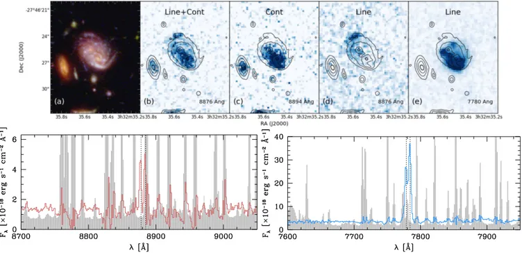
Figure 3. MUSE optical spectroscopy of the counterparts of ID.3 and ID.4. Top panels—(a) HST RGB image (see Figure2for details). (b) MUSE channel map at 8876 Ang, integrated over∼5 Å, showing the [OII] emission of the background component plus the starlight continuum from the two galaxies. The HST/F160W
contours are overplotted in black to guide the eye on the position of the sources.(c) MUSE channel map at 8894 Å, i.e., a few Å off the [OII] line, showing only the
continuum emission. The map is integrated over∼10 Å. (d) Difference between panels (b) and (d). The continuum emission is effectively subtracted, as confirmed by the disappearance of all thefield sources. The residual emission is the [OII] line emission from the background object, which thus resides at z=1.382 (consistent with
the CO redshift of ASPECS 3 mm.3). (e) Same as panel (d), but this time centered at 7780 Å, thus highlighting the [OII] emission of the foreground galaxy at
z=1.088. Bottom panels—MUSE optical spectra of the [OII] lines of the counterparts of ASPECS 3 mm.3 (left) and 3 mm.5 (right). The vertical dotted lines mark
the wavelengths corresponding to the[OII] doublet at z=zCO. The gray shading shows the noise in the spectra(which, at these wavelengths, is dominated by sky
ID.5(Figure13) and ID.8 (Figure14) lie in a crowded region of ourfield. Skelton et al. (2014) report a spectroscopic redshift z=1.047 for ID.5. However, the inspection of the MUSE data reveals two clearly distinguished line sets of the[OII] doublet at z=1.038 and z=1.098. The latter matches the redshift of two CO lines that are slightly too faint to be selected in our blind search(S/N≈4.8, see PaperI). ID.8, on the other hand, is found at another redshift (z=0.999). No CO emission is found at this position and frequency, although the lowest-J transition that we encompass is CO(4–3) at 1 mm. ID.8 is detected in the X-rays (Xue et al. 2011). Its faintness (F =8.2´10
-X 17 erg s−1cm−2, LX=4.3´1041 erg s−1)
seems consistent with a starburst rather than an AGN(Ranalli et al.2003).
ID.6 (Figure 13) is located ~ 4 east of ID.3 and probably belongs to a common physical structure (together with other galaxies with a spectroscopic z»1.09). It is detected in the
1 mm continuum, and its CO spectrum shows an∼3σ excess at the frequency of the expected CO(2–1) line. The CO(4–3) transition is also detected with similar significance, although the best Gaussian fit of the line suggests a velocity shift of ∼200 km s−1 between the two transitions. This is most likely
due to the poor S/N of the two lines.
ID.7(Figure14) appears as a very compact source ( =Re 0.7 kpc) at z=1.221. Its Chandra image reveals the presence of a bright AGN(FX=1.01´10-14erg s−1cm−2in Lehmer et al. (2005); 8.3´10-15erg s−1cm−2 in Evans et al. (2010);
´
-6.3 10 15 erg s−1cm−2 in Xue et al. 2011), yielding an
X-ray luminosity of LX=5.4´1043 erg s−1). It is not detected in the 1 mm dust continuum. A 3σ excess is measured at the expected frequency of the CO(2–1) transition.
ID.9 and ID.10 (Figure 15) are both at ~z 2.3. They are among the faintest galaxies in our sample in terms of LIR, just
above the 1011Lcut. ID.9 appears as a compact bulge. ID.10
appears as a spiral galaxy with disturbed morphology. ASPECS data cover three CO transitions in these galaxies: CO(3–2), CO(7–6), and CO(8–7). None of these lines are detected.
ID.11 (Figure 16) is a compact (Re=1.2 kpc) galaxy at
z=0.895. As for ID.8, the lowest-J CO transition in the ASPECS coverage is the CO(4–3), which remains undetected.
4. CO-BASED MEASUREMENTS 4.1. CO Luminosities and Associated H2Masses
We measure the line fluxes (or place limits) for all the CO transitions covered in both the 3 and 1 mm line scans. We extract the CO spectra at the position of the optical coordinates of the sources in our sample. We fit the lowest-J transitions accessible with ASPECS data with a Gaussian profile; in the case of a detection, wefit the higher-J lines imposing the same line width. We consider as detections those cases where the flux obtained in the Gaussian fit is >3×its uncertainty. If the line is not detected, we assume a fiducial line width of 300 km s−1 , and we use the upper boundary of the 3σ confidence range on the flux as upper limit. Table2reports the CO linefluxes, shifts compared with the nominal redshift, and the line width. The detected sources in our sample have a median CO flux of 0.19 Jy km s−1 (considering only the lowest-J transition observed in each object). For a comparison, the detected main-sequence galaxies in Tacconi et al. (2013) have a median COflux of 0.57 Jy km s−1, i.e., ´3 higher than the medianflux of our detections.
The luminosity of the lowest-J transitions observed in our molecular scans is transformed into the equivalent ground-state luminosity LCO 1 0¢ ( - ) using LCO¢ (J- -[J 1]) rJ1, where we adopt
the recent CO excitation ladder of main-sequence galaxies derived by Daddi et al. (2015): r21=0.76±0.09,
=
r31 0.42 0.07, and r41=0.310.06.30 The uncertainty
in LCO 1 0¢ ( - ) accounts for both the measured flux uncertainty
and the standard deviation in the rJ1 values in the sample
studied by Daddi et al.(2015). The molecular gas masses are then derived as a = ¢- - - M M r L K km s pc . 1 J J J H2 CO 1 1 1 2 ( ) ( [ ])
We adopt aCO = 3.6M(K km s−1pc2)−1 (Daddi et al.
2010b). This conversion factor has been demonstrated to be appropriate for main-sequence galaxies through comparisons with dynamical masses (Daddi et al. 2010b), CO line SED-fitting (Daddi et al. 2015), and detailed dust-SED modeling (Genzel et al. 2015). In Section 5.5 we further discuss the implications of our aCOassumption. Table3lists the values of
molecular gas masses that we derive for each source. We then combine these measurements or limits on the molecular gas mass with properties of the galaxies inferred from the SED
Table 2
CO Lines in the Galaxies of our Sample
ID Jup Dv Fline FWHM (km s−1) (Jy km s−1) (km s−1) (1) (2) (3) (4) (5) 1 3 −45±8 0.723-+0.0030.003 504±12 1 7 −150±120 0.786-+0.0060.006 504a 1 8 −45±70 1.098-+0.0050.005 504 a 2 2 135±9 0.443-+0.0070.007 538±13 2 5 135±45 0.502-+0.0900.090 538a 2 6 −45±45 0.820-+0.1000.100 538 a 3 2 −37±8 0.135-+0.0030.003 57±12 3 5 L <0.021 57a 4 2 52±7 0.180-+0.0060.006 82±11 4 4 L <0.121 82a 5 2 220±35 0.190-+0.0400.040 352±11 5 4 −28±40 0.390-+0.0650.065 352 a 6 2 −160±70 0.340-+0.0700.060 530±11 6 4 230±70 0.370-+0.0900.090 182 a 7 2 150±17 0.104-+0.0290.019 150±11 7 5 L <0.106 150a 8 4 L <0.059 L 9 3 L <0.076 L 9 7 L <0.012 L 9 8 L <0.230 L 10 3 L <0.048 L 10 6 L <0.144 L 10 7 L <0.465 L 11 4 L <0.015 L
Note.(1) Source ID. (2) Upper J of the CO transition. (3) Velocity shift, compared with the redshift quoted in Table1.(4) Line flux. (5) Line width, expressed as the full width at half maximum(FWHM) from the Gaussian fit.
aFixed from thefit of a lower J line.
30
Daddi et al.(2015) do not measure CO(4–3) in the galaxies in their sample. The value of r41adopted here is extrapolated from their measurements of r31
and r51, in the case of a CO ladder that peaks aroundJ»5(see their Figure 10,
fitting (in particular, the stellar mass M* and the SFR) to compute the molecular-to-stellar mass ratio MH2 M* and the
depletion timescaletdep=MH2 SFR(see Table3). 4.2. Size of the CO-emitting Region in ID.2
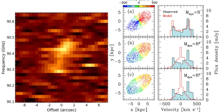
In the case of ID.2, our ALMA observations spatially resolve the CO(2–1) emission over >15 kpc, despite the relatively coarse spatial resolution of the 3 mm data. A clear velocity gradient is observed in the line emission, as shown in Figure4. While the resolution and the signal-to-noise ratio are too poor
for an accurate modeling of the gas dynamics, we obtain an estimate of the dynamical mass assuming that the gas is rotating in a disk with the inclination derived from the HST near-IR imaging (PA=−55°, inclination=60° with respect to the line of sight). We then assume a radial distribution of the mass that scales as MdynµRg, where γ=1 yields the flat
rotation curves typically observed in galaxies;γ=2 implies a constant surface density of mass in the disk, and yields
µ
vrot R ;andγ=3 corresponds to a solid rotator (vrotµR).
We then generated mock velocity maps for these three cases, assuming that the CO light traces the mass distribution; and we Table 3
CO Luminosities and CO-based Galaxy Parameters
ID z Jup L¢ LCO 1¢ (-0) MH2 MH2 M* tdepl ´109 ( Kkm s−1pc2) (´109Kkm s−1pc2 ) (´109M) (Gyr) (1) (2) (3) (4) (5) (6) (7) (8) 1 2.543 3 24.03-+0.100.10 57-+1010 206+-3434 12-+22 3.3-+0.60.7 2 1.551 2 13.71-+0.270.21 18-+22 65+-88 0.24-+0.050.05 0.9-+0.40.6 3 1.382 2 3.364-+0.080.07 4.4-+0.50.5 15.9+-1.91.9 0.30-+0.070.08 0.9-+0.30.6 4 1.088 2 2.831-+0.090.09 3.7-+0.50.5 13.4+-1.71.7 0.48-+0.110.13 0.6-+0.30.4 5 1.098 2 3.089-+0.660.70 4.1-+1.01.0 15-+44 2.5-+0.60.7 0.33-+0.090.09 6 1.094 2 5.388-+1.160.91 7.1-+1.71.5 25+-65 0.34-+0.090.10 1.6-+0.70.9 7 1.221 2 2.047-+0.570.37 2.7-+0.80.6 10-+32 0.6-+0.20.16 0.066-+0.0200.016 8 0.999 4 <0.20 <0.63 <2.3 <0.03 <0.06 9 2.447 3 <2.4 <5.6 <21 <8 <1.8 10 2.224 3 <2.2 <5.3 <19 <1.6 <0.9 11 0.895 4 <0.53 <1.7 <6.2 <0.4 <0.15
Notes.(1) Source ID. (2) Redshift. (3) Observed transition. (4) Line luminosity. (5) Equivalent CO(1–0) luminosity, assuming the rJ1ratios in Daddi et al.(2015). (6)
Molecular gas mass, assuming aCO= 3.6M(Kkm s−1pc2)−1.(7) Molecular-to-stellar mass ratio,MH2 M*.(8) Depletion time,tdep=MH2 SFR.
Figure 4. Left panel: position–velocity diagram of the CO(2–1) emission in ID.2, extracted along the major axis of the galaxy. A velocity gradient is apparent. Right panel: simulated velocity maps of ID.2, assuming that the gas is emitted in a disk geometry and that the CO(2–1) emission traces the mass distribution. The three models refer to different radial scalings of the dynamical mass:(a)MdynµR (thus vrot=const); (b)MdynµR2(i.e., constant surface mass density in the disk;
µ
vrot R); (c) MdynµR3 (i.e., constant volume mass density; vrotµR, i.e., solid rotator). All models assume a dynamical mass Mdyn=2´1011 M at
R=8.3 kpc. The expected line profiles (red histograms) are compared with the observed one (black dots). The flat rotation curve model seems to best reproduce the observed line profile.
inferred expected line profiles (see Figure4). The γ=1 case shows the typical “double-horned” profile observed in local spiral galaxies. This seems to provide a better description of the observed CO(2–1) line than the other two models, which fail to reproduce the extension of the blue wing of the line. The implied dynamical mass is Mdyn»2´1011M at
R=8.3 kpc (=the effective radius). We stress, however, that this estimate is highly dependent on the model assumptions. A firmer estimate of the dynamical mass in this galaxy requires deeper data at higher spatial resolution.
ID.2 also appears in the SINFONI Integralfield spectroscopy survey in the near-IR (SINS; Förster Schreiber et al. 2009) as GMASS-1084(see also Kurk et al.2013). SINS investigated the morphology and kinematics of ionized gas(as traced by the Hα hydrogen line) in a sample of galaxies at =z 1 3.5– . The Hα line in ID.2 is emitted on a smaller region (half-light radius
=
R1 2 3.1 1.0kpc) than the CO. The observed Hα circular velocity is 67±9 km s−1, which is corrected into 230 km s−1by assuming a low-inclination angle (~ 20 ). This yields a dynamical mass of1.2´1011
M , roughly consistent with our estimate, especially if one considers that the high level of dust reddening (AV=2.4 mag from our global MAGPHYS fit) in
this source may be responsible for suppressing Hα in parts of this galaxy. We note, however, that the SEDfit of this source in Förster Schreiber et al. (2009) yields a stellar mass of only
* = -+ ´ M 3.61 0.60 10 0.34 10 M and a high SFR=490-+31 190 M yr−1 (i.e., LIR »5.7´1012 L). This last estimate disagrees with
our dust continuum measurements: e.g., assuming a modified blackbody template withβ=1.6 andTdust =25K, such a high SFR would imply a dust-continuum flux density of 11 mJy at 1.2 mm (observed: 0.22 ± 0.02 mJy) and of 32 mJy at 160 μm (observed: 6.9 ± 0.3 mJy).
As seen from Figure4, the molecular gas, as traced through CO emission, is extended on scales of >15 kpc (> 2 at z=1.552), i.e., comparable to that of the stellar disk. On the other hand, the 1 mm dust continuum is unresolved at
´
1.5 1.0 resolution, i.e., it is significantly smaller than that of the CO (see Figure 11). This is not an effect of interferometric filtering or sensitivity of the 1 mm data. When we convolve the 1 mm continuum data to the synthesized beam of the 3 mm data, we do not recover the size seen in CO emission. This serves as a cautionary note that CO and dust sizes may not be the same. As a consequence, the masses deduced from these measurements may trace different regions or components in the galaxy(for other examples of a mismatch between CO and dust morphology in high-redshift galaxies, see Riechers et al. 2011; Hodge et al. 2015; Spilker et al. 2015). This may explain some of the differences between gas mass estimates derived from CO and dust imaging, with the gas masses derived from dust emission being typically lower than those derived from CO (see Section 5.5): At the observed wavelength (1.2 mm), dust is optically thin (with the only exception of ID.1, all the sources in our sample globally have Sgas 104Mpc−2, i.e., NH21024cm−2; this yields τ
[242 GHz] 0.1 for solar metallicities, adopting the Draine & Lee 1984 formalism). The CO low-J emission, on the other hand, is optically thick practically everywhere in galaxies.
4.3. CO Excitation
As shown in Table 1, ASPECS covers 2–3 different CO transitions in 9 out of 11 galaxies in our sample. Figure 5 shows the inferred constraints on the CO excitation ladder. In
ID.1, all three observed transitions [CO(3–2), CO(7–6), and CO(8–7)] were detected in our blind search for line emission (ASPECS 3 mm.1, 1 mm.1, and 1 mm.2, respectively). In ID.2, the CO(2–1) line appears in the results of our blind search (ASPECS 3 mm.2). The CO(5–4) and CO(6–5) lines are also observed, but because of their lower significance, they were not detected in our blind search. In particular, the CO(6–5) line is very noisy, as it is found at the high-frequency end of the 1 mm spectral scan, and it is spatially located at the edge of our mosaic. The CO(2–1) transitions in ID.3 and ID.4 are also identified in our blind search (ASPECS 3 mm.3 and 3 mm.5, respectively). However, the CO(5–4) line in ID.3 and the CO(4–3) line in ID.4 are not detected. In particular for ID.3, this places very strong limits on the CO excitation of this galaxy, significantly below the average CO ladder of the Milky Way disk (see Figure 5). In ID.5 and ID.6, we detect both CO(2–1) and CO(4–3). Finally, in ID.7 we only have a tentative detection of CO(2–1), while the CO(5–4) transition remains undetected. No other line is detected in the remainder of our sample.
In Figure5we compare our measurements and limits with the CO excitation templates of the Milky Way disk, and of the starburst in M82(Weiß et al.2007). Additionally, we compare with the average template for high-z main-sequence galaxies by Daddi et al.(2015) and with the theoretical predictions based on the SFR surface density by Narayanan & Krumholz(2014) (see Table1and the discussion in Section 5.2.2). In no case do we find starburst-like CO excitation that would be comparable with Figure 5. CO ladder for the galaxies of our sample detected in CO. Filled symbols mark the transitions detected in our blind search(see PaperI), while empty symbols mark lines that do not match the blind detection requirements. Upper limits, marked with triangles, correspond to 3σ limits. The excitation templates of the Milky Way and M82 are taken from Weiß et al.(2007), while the main-sequence galaxy template is from Daddi et al.(2015) (D15). Finally, the theoretical predictions based on the SFR surface density are based on Narayanan & Krumholz(2014) (NK14). All templates are scaled to match the observed COflux of the lowest J transition detected in ASPECS. The galaxies in our sample typically show a modest to very low CO excitation. ID.1 (=ASPECS 3 mm.1, 1 mm.1, 2) and ID.5 show slightly higher CO excitation than the template by Daddi et al.(2015), although still well below the high-excitation case of the M82 starburst template.
the center of M82(Weiß et al.2007) or with what is typically observed in high-z sub-mm galaxies (SMGs; e.g., Bothwell et al.2013; Spilker et al.2014). ID.1 shows a CO(7–6)/CO(3–2) ratio r73=0.2, consistent with a high-density photon-dominated
region(Meijerink et al.2007). On the other hand, the CO(8–7) transition appears brighter, implying that a high-excitation component of the interstellar medium (ISM) might be in place. Interestingly, ID.2 shows a lower excitation(in particular in the CO[5–4]/CO[2–1] ratio, which is consistent with Milky Way excitation). This difference in CO excitation is remarkable when we consider that ID.1 is not detected with Chandra (LX<6´1042 erg s−1), whereas ID.2 shows a bright X-ray detection, indicative of the presence of a central AGN. The X-ray emission from the AGN can boost the emission of high-J CO transitions. The CO(7–6)/CO(3–2) ratio r73 is typically
0.16–0.63 in high-density photon-dominated regions that are powered by star formation(as in ID.2), but it can reach values as high as r73=30 in the presence of intense X-ray illumination
(Meijerink et al. 2007). This might explain the higher CO excitation observed in high-z QSOs with respect to submilli-meter galaxies (Carilli & Walter2013). The lack of such high-excitation feature suggests that the central AGN activity in ID.2 has no major impact on its global CO properties. We attribute the higher excitation in ID.1 to the much more compact emission in this galaxy. As shown in Table1, ID.1 has a radius that is only ∼1/5 of that of ID.2, which translates into a difference in surface area of ∼24. Our MAGPHYS-based SFR estimates are comparable (∼70Myr−1), thus the surface density of star
formation(SSFR) is much higher in ID.1. This is also discussed
in Section 5.2 below. The increased radiation field intensity caused by the high SFR surface density and/or the higher gas density are very likely the reason for the increased CO excitation (see Narayanan & Krumholz2014).
5. DISCUSSION
In the following we discuss the sources of our sample in the broad context of gas properties in high-redshift galaxies.
5.1. Location in the Galaxy “Main-sequence” Plot The stellar masses of the galaxies in our sample range between(2.8 275– )´109
M (two orders of magnitude). The
>
LIR 1011Lcut in our sample definition selects sources with
SFR>10Myr−1. The measured SFRs range between
12–150Myr−1.31
Figure1shows the location of our galaxies in theM*–SFR
(“main sequence”) plane. We plot all the galaxies in the field with an F850LP or F160W magnitude brighter than 27.5 mag (this cut allows us to remove sources with highly uncertain SED fits). The galaxies in the present sample are highlighted with large symbols. The different redshifts of the sources are indicated by different colors. As expected from the known evolution of the“main sequence” of star-forming galaxies (e.g.,
Whitaker et al.2012; Schreiber et al.2015), sources at higher redshifts tend to have a higher SFR per unit stellar mass. Comparing with the Herschel-based results by Schreiber et al. (2015), we find that half of the galaxies in our sample (ID.1, 2, 4, 8, 9, 10) lie on the main sequence (within a factor ´3 ) at their redshift. Three galaxies (ID.5, 7, 11) are above the main sequence (in the “starburst” region), and the remaining two galaxies(ID.3 and ID.6) show an SFR ~ ´3 lower than main-sequence galaxies at these redshifts and stellar masses. Similar conclusions are reached when we compare our results with the main-sequencefits by Whitaker et al. (2012) (see Figure1).
5.2. Star Formation Law
The relationship between the total infrared luminosity(LIR, a
proxy for the SFR) and the total CO luminosity ( ¢LCO, a proxy
for the available gas mass) of galaxy samples is typically referred to as the “integrated Schmidt–Kennicutt” law (Schmidt 1959; Kennicutt1998; Kennicutt & Evans2012), or, more generally, the “star formation” law. Sometimes average surface density values are derived from these quantities, resulting in average surface SFR densities(SSFR) and gas densities (Sgas). We here
explore both relations.
5.2.1. Global Star Formation Law: IR Versus CO Luminosities In Figure6we compare the IR and CO(1–0) luminosities of our sources with respect to a compilation of galaxies both at low and high redshift from the review by Carilli & Walter (2013), and with the secure blind detections in Decarli et al. (2014). For galaxies in our sample that are undetected in CO, we plot the corresponding 3σ limit on the line luminosities. The IR–CO luminosity empirical relation motivates the LIR cut in
our sample selection, as galaxies with LIR >1011 L should
have CO emission brighter than L¢ »3´109 Kkm s−1pc2
(i.e., our typical sensitivity limit in ASPECS; see PaperI). All the galaxies in our sample should therefore be detected in CO. Wefind that most of the CO-detected galaxies in our sample lie along the one-to-one relation, followed by local spiral galaxies as well as color-selected main-sequence galaxies at1< <z 3 (Daddi et al. 2010b; Genzel et al. 2010, 2015; Tacconi et al. 2013). Only two galaxies significantly deviate: ID.5, which appears on the upper envelope of the IR–CO relation, close to high-redshift starburst galaxies; and ID.7, which is largely underluminous in CO for its bright IR emission. As discussed in the previous section, these two galaxies appear as starbursts in Figure1. Moreover, ID.7 hosts a bright AGN. If the AGN contamination at optical wavelengths is significant, then our MAGPHYS-based SFR estimate is likely in excess (since MAGPHYS would associate some of the AGN light at rest-frame optical and UV wavelengths to a young stellar population), thus explaining the large vertical offset of this galaxy with respect to the “star formation law” shown in Figure 6. Notably, out of the 4 CO non-detections in our sample, ID.9 and ID.10 are still consistent with the relation, while ID.8 and ID.11 are not. These two galaxies are located at z=0.999 and z=0.895, respectively. The lowest-J transition sampled in our study is CO(4–3). Their non-detections might be explained if the excitation in these two sources were much lower than what we assumed to inferLCO 1 0¢ ( -) ( =r41 0.31;see
Section4.1).
The sources that are also detected in the blind search for CO (ID.1, 2, 3, 4) tend to lie on the lower “envelope” of the plot.
31
We note that the FAST analysis by Skelton et al.(2014) yields consistent SFRs for ID.1, ID.3, and ID.10, but different values(by a factor ´2 or more) for ID.2 (6M yr −1), ID.4 (50M yr −1), ID.5 (21M yr −1), ID.6
(3.7M yr −1), ID.7 (230M yr −1), ID.8 (0.01M yr −1), and ID.11
(2.6M yr −1). No FAST-based SFR estimate is available for ID.9. These
differences are most likely due to (1) different assumptions on the source redshifts;(2) different coverage of the SED photometry, in particular thanks to the addition of the 1 mm continuum constraint in our MAGPHYS analysis;(3) different working assumptions in the two codes. In particular, FAST relies on relatively limited prescriptions for the dust attenuation and star formation history, and does not model the dust emission.
This is expected, as these galaxies have been selected based on their CO luminosity(x-axis).
Figure6also shows the x-axis position of the remaining CO blind detections from the 3 mm search in Paper I. The CO luminosities of these lines are uncertain (the line identification is ambiguous in many cases, and a fraction of these lines is expected to be a false positive; see Paper I); however, it is interesting to note that these sources typically populate ranges of line luminosities that were previously unexplored at z>1 (see similar examples in Chapman et al. 2008, 2015b; Casey et al.2011), and comparable with or even lower than the typical dust luminosities of local spiral galaxies. We emphasize that a significant fraction of these lines is expected to be real (see PaperI). Deeper data are required to better characterize these candidates.
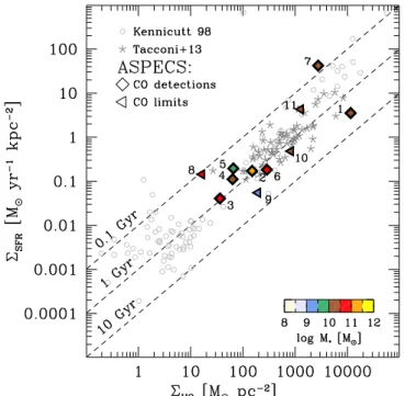
5.2.2. Average Surface Densities: SFR Versus Gas Mass We infer average estimates of SSFR and Sgasby dividing the
global SFR and MH2of the galaxy by afiducial area set by the
size of the stellar component, as CO and optical radii are typically comparable(Schruba et al.2011; Tacconi et al.2013). We thus use the information from the stellar morphology derived by van der Wel et al.(2012) and reported in Table1to infer SSFR=SFR/( p R2 e2) and SH2=MH2/( p R2 e2), where
MH2is our CO-based measurement of the molecular gas mass,
and the factor 2 is due to the fact that the Reincludes only half
of the light of the galaxy(see a similar approach in Tacconi et al.2013).
In Figure 7 we show the star formation law for average surface densities. Global measurements of local spiral galaxies and starbursts are taken from Kennicutt(1998), and corrected for the updated SFR calibration following Kennicutt & Evans (2012) and to the aCOvalue adopted in this paper. We also plot
the galaxies in the IRAM Plateau de Bure HIgh-z Blue Sequence Survey (PHIBSS; Tacconi et al. 2013), again corrected to match the same aCO assumption used in this
work, and the secure detections in Decarli et al. (2014). Interestingly, the two CO-brightest galaxies in our sample, ID.1 and ID.2, appear to populate opposite extremes of the density ranges observed in high-z galaxies: ID.1 appears very compact, thus reaching the top right corner of the plot (S » 10,000gas
M pc−2). On the other hand, in ID.2 the vast gas reservoir is spread over a large area(as apparent in Figure4), thus yielding a globally low Sgas. We alsofind that most of the sources in our
sample lie along thetdepl»1 Gyrline, in agreement with local spiral galaxies and the PHIBSS main-sequence galaxies. Only ID.7 and ID.8 lie closer to the tdepl»0.1 Gyr line. In particular, the offset of ID.7 with respect to the bulk of the sample in the context of the global star formation law(Figure6) is combined here with the very compact size of the emitting region, thus isolating the source in the top left corner of the plot Figure 6. IR luminosity as a function of the CO(1–0) luminosity for both local
galaxies (gray open symbols) and high-redshift sources ( >z 1, gray filled symbols) from the compilation in Carilli & Walter (2013). The sources in our sample are shown with large symbols, using the same coding as in Figure1. In addition, we also plot the x-axis position of the remaining CO lines found in our 3 mm blind search (downward triangles; see PaperI). The two parallel sequences of“normal” and “starburst” galaxies (Daddi et al.2010b; Genzel et al. 2010) are shown as dashed lines (in gray and red, respectively). Our sources cover a wide range of luminosities, both in the CO line and in the IR continuum. Most of the sources in our sample lie along the sequence of“main sequence” galaxies. Four sources lie above the relation: ID.5, which still falls close to the high-z starburst region; ID.7, in which the AGN contamination may lead to an excess of IR luminosity; and ID.8 and ID.11, which are undetected in CO, and which might be shifted toward the relation if we assumed very low CO excitation(as observed in other galaxies of our sample). Conversely, most of the sources detected in CO in our blind search (see Paper I) that lack an optical/IR counterpart lie significantly below the observed relation.
Figure 7. The “global” star formation law relates the average star formation rate surface density(SSFR) with the average gas density in galaxies. Here we
consider only the molecular gas phase(SH2). Each point in the plot refers to a
different galaxy. We plot the reference samples from Kennicutt (1998) (corrected for the updated SFR calibration in Kennicutt & Evans2012), as well as the PHIBSS galaxies from Tacconi et al.(2013). Data from the literature have been corrected to match the same aCO= 3.6 M(Kkm s−1pc2)−1
assumed in this work. The symbol code is the same as in Figure6. The galaxies in our sample align along thetdepl»1 Gyr, with the only exception of ID.7 and ID.8, which show a short depletion time. It is interesting to note that the two CO-brightest galaxies in our sample, ID.1 and ID.2, populate opposite extremes of the high-z galaxy distribution, with the former being very compact (thus displaying higher SFR and gas densities), and the latter being very extended(thus showing lower SFR and gas densities).
(see Figure7). Once again, a significant AGN contamination in the estimates of both the rest-frame optical/UV luminosity and in the size of the emitting region could explain such an outlier. We also caution that, in some of these galaxies, optical and CO radii might differ.
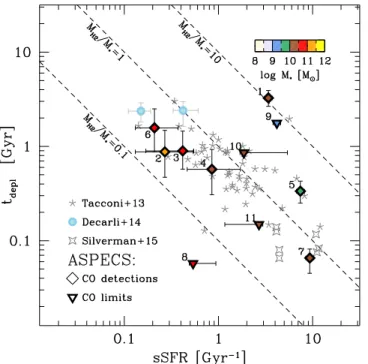
5.3. Depletion Times
Figure 8 shows the depletion time, tdepl=MH2 SFR, as a function of the specific SFR. This timescale sets how quickly the gas is depleted in a galaxy given the currently observed SFR (ignoring any gas repleneshing). Our data are compared again with the secure blind detections in Decarli et al. (2014), with the PHIBSS sample, and with the sample of starburst galaxies studied by Silverman et al. (2015) (in the latter case, we do not change the adopted value of
aCO= 1.1 M(Kkm s−1pc2)−1, as these are not main-sequence galaxies). Starburst galaxies tend to reside in the bottom right corner of the plot (they are highly star forming given their stellar mass, and they are using up their gaseous reservoir fast). Galaxies with large gas reservoirs and mild star formation populate the top left corner of the plot. Since the IR luminosity is proportional to the SFR and the CO luminosity is used to infer MH2, the y-axis of this plot conceptually
corresponds to a diagonal line (top left to bottom right) in Figure6. In addition, the diagonal lines in Figure8 mark the loci of the constant molecular-to-stellar mass ratio MH2 M*.
The sources in our sample range over almost 2 dex in sSFR and tdepl. Noticeably, ID.1 is highly star forming (it resides
slightly above the main sequence of star-forming galaxies at ~
z 2.5, see Figure1), so we would expect it to reside in the bottom right corner of Figure8; however, its gaseous reservoir is very large for its IR luminosity (see also Figure 6), thus
placing ID.1 in the top right corner of the plot(MH2 M* = 12). On the other hand, ID.2 hosts an enormous reservoir of molecular gas, but because of its even higher stellar mass (yielding low sSFR), it resides on the left side of the plot (MH2 M* =0.24). Their depletion timescales, however, are comparable(1–3 Gyr). We stress that these results are based on very high S/N CO line detections, and on very solid descriptions of the galaxy SEDs(see Figure11). The sources that populate the starburst region in Figure1and reside in the top left part of Figure 6 (in particular, ID.5 and ID.7) consistently appear in the bottom right corner of Figure8, that is, among starbursts.
5.4. Gas-to-Stellar-Mass Ratios
A useful parameter to investigate the molecular gas content in high-z galaxies is the molecular gas to stellar mass ratio,
*
MH2 M . We prefer this parameter rather than the molecular
gas fraction, fgas =MH2 (M*+MH2), as the two involved
quantities(MH2and M*) appear independently at the numerator
and denominator of the fraction, so that the parameter is well defined even when we only have upper limits on MH2. Figure9
shows the dependence ofMH2 M*on redshift in the galaxies of
our samples and in galaxies from the literature. This plot informs us of the typical gas content as a function of cosmic time, and can help us shed light on the origin of the cosmic star formation history (see, e.g., Geach et al. 2011; Magdis et al. 2012, and Paper III of this series). Color-selected star-forming galaxies close to the epoch of galaxy assembly are Figure 8. The depletion timetdepl=MH2SFRas a function of the specific star
formation rate sSFR=SFR/ *M for the galaxies in our sample, the secure
blind detections in Decarli et al.(2014), the PHIBSS sample by Tacconi et al. (2013), and the starburst sample in Silverman et al. (2015). The symbol code is the same as that in Figure6. Starburst galaxies typically reside in the bottom right corner of the plot. Our ASPECS sources cover a wide range in parameter space, highlighting the diverse properties of these galaxies.
Figure 9. Gas mass fraction (defined asMH2 M*) as a function of redshift from
various samples of galaxies in the literature(gray, from the compilation in Carilli & Walter2013), compared with the secure CO detections in Decarli et al.(2014), the PHIBSS sample (Tacconi et al.2013), the starburst sample in Silverman et al.(2015), and our results from this work. The symbol coding is the same as in Figure1. Our data seem to support the picture of a generally increasingMH2 M*ratio in main-sequence galaxies as a function of redshift, as
highlighted by the fgas =0.1´(1+z)2 green line (Geach et al. 2011;
Magdis et al.2012). In particular, ID.2 appears as a starburst with respect to its position above the“main sequence” in Figure1, and shows a highMH2 M*
ratio. On the other hand, we also point out that significant upper limits are present(triangles).
claimed to show largeMH2 M*, with reservoirs of gas as large
as(or even larger than) the stellar mass (i.e.,MH2 M* ~ 1;see, e.g., Daddi et al.2010a; Tacconi et al.2010,2013). Indeed, we find examples of very high gas fractions: ID.1 (MH2 M* =12) and the starburst galaxy ID.5 (MH2 M* = 2.5) are the most extreme cases. However, it is interesting to note that we also find galaxies with very modest gas fractions, such as ID.2 (MH2 M* =0.24). The CO-detected galaxies at1.0< <z 1.7 in our sample show an average MH2 M* ratio that is ~ ´2
lower than the average value for the PHIBSS sample at the same redshift, and closer to the global trend established in Geach et al.(2011) and Magdis et al. (2012). The non-detection of CO in ID.8 places particularly strict limits (MH2 M*<
0.03). If the lack of detection is attributed to the very low CO excitation in this galaxy, then it would take a 10×lower r41
(i.e.,r41»0.03) to shift ID.8 on the average trend reported by Geach et al.(2011).
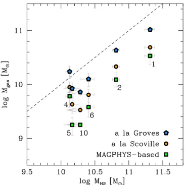
5.5. CO versus Dust-based ISM Masses
In addition to the CO line measurements, 6 of the 11 galaxies in our sample also have detections in the 1 mm dust continuum. We can thus estimate the mass of the molecular gas independently of the CO data. The Rayleigh–Jeans part of the dust emission is only weakly dependent on the dust temperature, thus it can be used to trace the mass of dust. Using the dust-to-gas scaling (see, e.g., Sandstrom et al. 2013), it is possible to infer the gas mass via the dust mass.
Groves et al.(2015) compare CO-based gas masses with the monochromatic luminosity of the dust continuum in the Rayleigh–Jeans tail. Their analysis relies on a detailed study of 37 local spiral galaxies in the KINGFISH sample(Kennicutt et al. 2011). The galaxy luminosity in the Herschel/SPIRE 500μm band is found to scale almost linearly with the gas mass, yielding n m = n M M L L 10 28.5 500 m 10 . 2 gas 10 10 ( ) ( ) We compute the rest-frame luminosity nLn(500 μm) from the
observed 1 mm continuum of the galaxies in our sample. For the k-correction, we adopt a modified blackbody with
Tdust=25 K and β=1.6 (see, e.g., Beelen et al.2006), shifted
at the redshift of each source. Since the observing frequency (242 GHz) falls close to the rest-frame 500 μm (as most of our
sources reside atz~1.2), and we are sampling the Rayleigh–
Jeans tail(which is almost insensitive to the dust temperature), the differences in the corrections due to the adopted templates are negligible for the purposes of this analysis. The adopted values for the k correction, as well as the resulting gas masses, are listed in Table4.
A similar approach was presented by Scoville et al. (2014,2016). This calibration is tuned on a set of relatively massive[(0.2 4– )´1011
M ] star-forming galaxies (30 local
star-forming galaxies, 12 low-redshift ultraluminous IR galaxies (ULIRGs), and 30 SMGs at z=1.4–3.0), all having literature observations of the CO(1–0) transition. The tight relation observed between CO(1–0) luminosity and the rest-frame 850μm monochromatic luminosity (see Figure 1 in Scoville et al.2016) suggests that a simple conversion factor can be used to derive gas masses from monochromatic dust continuum observations. By setting the dust temperature to
=
Tdust 25K(following Scoville et al. 2014), we derive from Equation(12) in their paper MISMfrom our 1 mmflux densities
as follows: ⎜ ⎟ ⎛ ⎝ ⎞⎠ ⎛ ⎝ ⎜ ⎞ ⎠ ⎟ n = + G G n - M M z F D 10 1.20 1 mJy 350 GHz Gpc , 3 ISM 10 4.8 3.8 0 RJ L 2 ( ) ( ) where Fν is the observed dust continuum flux density at the observing frequency ν (242 GHz in our case), DL is the
luminosity distance, and GRJis a unitless correction factor that
accounts for the deviation from the n2scaling of the Rayleigh–
Jeans tail. In the reference sample of local galaxies, low-redshift ULIRGs, and high-z SMGs that Scoville et al.(2014) used to calibrate Equation(3), G = G = 0.71RJ 0 . The resulting
ISM masses are listed in Table4.
Finally, we can infer an estimate of Mgasfrom the estimate of
the dust mass, Mdust, that we obtain via our MAGPHYSfit of
the available SED, simply scaled by afixed dust-to-gas mass ratio(DGR). Sandstrom et al. (2013) investigate the dust and gas content in a sample of local spiral galaxies and find DGR≈1/70. Genzel et al. (2015) and Berta et al. (2016) perform a detailed analysis of both gas- and dust-mass estimates in galaxies at0.9< <z 3.2 observed with Herschel, andfind a lower value of DGR≈1/100, which is the value we adopt here. We stress that there is a factor > ´2 scatter in the Table 4
Gas Mass Estimates Based on the Dust Continuum
ID z Fn(1.2mm) k-corr log Mgas,Groves log MISM,Scoville log Mgas,MAGPHYS
(μJy) (M) (M) (M) (1) (2) (3) (4) (5) (6) (7) 1 2.543 552.7±13.8 0.374 11.02-+0.0110.011 10.69-+0.0110.011 10.53-+0.170.17 2 1.551 223.1±21.6 0.919 10.63-+0.040.04 10.33-+0.040.04 10.09-+0.140.13 4 1.088 96.5±24.7 1.665 10.24-+0.100.13 9.95-+0.130.10 9.78-+0.200.18 5 1.098 46.4±14.9 1.641 9.93-+0.120.17 9.63-+0.170.12 9.25-+0.190.14 6 1.094 69.6±18.9 1.650 10.10-+0.100.14 9.81-+0.140.10 9.58-+0.180.17 10 2.224 36.7±13.8 0.478 9.86-+0.140.20 9.53-+0.200.14 9.25-+0.200.17
Note.Only sources detected at 1 mm in ASPECS are considered. (1) Source ID. (2) Redshift. (3) Observed 242, GHz=1.2, mm continuum flux density (see Paper II). (4) k correction, expressed as the ratio between the flux density computed at lrestframe= 500μm and the one at lobs= 1.2 mm, assuming a modified blackbody
template for the dust emission withβ=1.6 andTdust=25K.(5) Gas mass based on the 1 mm flux density, derived following Equation (2) (Groves et al.2015). (6) Gas mass based on the 1 mmflux density, derived following Equation (3) (Scoville et al.2014,2016). (7) Gas mass derived from the dust-mass estimate resulting from MAGPHYS SEDfitting, assuming a dust-to-gas ratio DGR=1/100.