Modeling an assembly line for configuration and flow management

(1)

ELSEVIER

Cbmprrter Intqratrd Manufumnrr~ .Svsrem\ Vol. I I. No. I--?, p. 15-24, IYYX 6: lYY8 I~lxxer Science Ltd. All right9 rcsavcd

Printed in ?ireat Bntan I195 I-524WYX $ -~ xc front matlcr

PII: SO951-5240(98)00005-6

Modeling an assembly line for

configuration and flow management

M Lucertini$, D Pacciarelli+ and A Pacifici

“Dipartimento di Informatica, Sistemi e Prod&one, Universitti ‘Tor Vergata: Roma, Italy

‘Dipartimento Discipline Scientifiche: Chimica e Informatica, Universit’a di Roma Tre, Roma, Italy

In its basic form the management control of a flexible production system requires to assign a set of operations to a set of machines, and to connect machines by a transporta- tion network, such that a number of constraints is satisfied and some efficiency index is optimized. The aim of the work is to give a general framework to formulate and model, in a formal way, different subproblems arising from embedding an assembly process on different configurations of a flexible production system. Because of the complexity of the overall problem, it is useful to have simple and well structured layouts and procedures that help the design and operation of flexible systems. These layouts and procedures induce additional constraints, due to the products’ and the process’ features. The paper also investigates the complexity of various subcases of the problem. 0 1998 Elsevier Science Ltd. All rights reserved

Keywords: flexible assembly systems, combinatorial optimization

Introduction weights correspond to the time needed to perform

Flexible Assembly Systems (FAS) are a class of automated systems which can be used to improve productivity in discrete parts manufacturing. For some contributions on manufacturing models see, for example’. In its basic form an FAS consists of a finite set of operations, each having a processing time and a set of precedence constraints among operations, a set of machines performing operations and a transportation network. A transportation network can be modeled as a set of positions in which machines can be placed, and a set of connections allowing parts to be moved from one machine to another. Because of the complexity of these systems, it is useful to have simple and well structured layouts and procedures that help the design and operation of FASs. These layouts and procedures induce additional constraints, due to the products and the processes features. A set N of n operations with the corresponding set A of precedence constraints can be represented as a weighted acyclic graph G(N, A) (in the following Assembly Graph), usually a tree, where the node

the operations (assumed to be the same indepen- dently on the machine used). When an assembly graph is embedded in a plant layout, with all its different types of constraints (placement, transportation, size, weight, information flow, computational, etc.), even the relatively simple structure of the tree may produce complex material flow patterns. Usual efficiency indicators (throughput, completion time, part transfers, workload balance, etc.) become difficult to evaluate and even to be formulated in logical terms or as the optimal solution of a decision problem expressed in analytical form.

The problem considered is the following: given an assembly graph, a set of machines and a transportation network, find the assignments of operations to machines and machines to physical positions, the routing of the units among machines and the sequencing of operations on each machine, such that a suitable objective function is minimized (number of part transfer, completion time, cycle time, workload balance). This problem generalizes several widely known relevant problems in production optimization:

*Corresponding author. the well known assembly line balancing problem

(2)

16 Modeling an assembly line for conjiguraion and flow management: M Lucertini et al.

@LB), the tooling, and several routing and scheduling problems. In particular, ALB is a traditional problem in industrial engineering and has been, since the first formulation by Hengelson et al. in 19542, the subject of a great number of papers. ALB falls into the class of NP-hard problems”, therefore most of the research efforts have been made to develop efficient heuristics solving large scale ALB problems (see for example4x5). As shown in Chase’s survey6 and more recently in7, ‘in spite of hundreds of works on assembly lines, only a little number of companies utilizes published techniques to balance their lines’, as in’. One of the reasons for this fact is that the models usually adopted to solve the problem suffer from substantial loss of information. In fact, little work has been done on modeling the full range of practical considerations in designing assembly lines. Moreover, the most common performance indices for this problem are the makespan and cycle time, whereas other factors may also heavily affect system performances. Some of these, such as traffic problems, transportation network congestion and set-up costs are often considered as marginal in Material Flow Management and in Assembly Line Balancing. There are a lot of meaningful cases in which the transportation network becomes the real bottleneck of the plant, due to inefficient part flow management procedures’. The part transfer minimization corresponds to a surrogate for taking into account both traffic problems and set-up costs. Other possible indices for taking into account traffic problems are the number of links in the transportation network needed to satisfy all the material flow requirements, or the existence of particular structures in the transportation network which are ‘difficult’ to manage, such as cycling of parts in the system.

The aim of this paper is to analyze several widely used architectures and material flow policies, to point out some properties useful to design decision rules and to evaluate the corresponding optimal@ bounds. In the next section we introduce the notation and a numerical example. In particular we show that a solution resulting from a compromise taking into account both production rate and traffic problems could be more attractive than the one obtained by maximizing just one of these two objectives. Then we give a formal statement of the problem in an optimization format. In a later section we will present some general properties concerning the feasibility of a solution, given certain partial decisions. In a later section we deal with the problem of optimally assigning operations to physical machines located in specified positions.

Statement of the problem

In this section we introduce the notation and give a formal statement of the problem in an optimization format.

Problem data

Acyclic assembly graph: G(N, A), where N is the set of n assembly and/or manufacturing operations. If arc (i, j)~ A then a machine k is allowed to perform operation j only when the subassembly resulting from operation i is available on machine k. Hereafter in the paper it is assumed that, if no precedence relationship exists between i and j, these operations are performed on different subassemblies and can be executed in parallel.

Set of machines: M, there are m multipurpose flexible workstations M= 1, 2, . . . m in the following denoted as ‘machines’. A machine k E A4 can execute only one operation at a time, preemption is not allowed. In the case of flexible machines we assume that the tooling is decided a priori, given the assembly graph, and no reconfiguration is allowed during the running of the production process, this case is referred to in literature as static tool alloca-

tion, see for example”. Therefore each machine can

perform a fixed subset of all the operations.

Graph of existing physical connections: E(P, C). P

is the set of positions where a machine can be placed. A directed arc (i, j) exists if and only if there is a physical connection from position i to position j.

Decision variables

Partition of operations in subsets assigned to the machines: TC = {S,, &, . . . S,}, with 71 E II; II set of feasible partitions. In the following it is assumed that each operation can be performed by a fixed subset of machines and II is simply given as the set of all partitions such that each operation is assigned to an allowed machine. Given x, each S, corresponds to a completely specified machine k. In the following, to simplify the notation, S, also denotes the subgraph of G induced by the corresponding subset of operations. Furthermore, a partition rr = {S1, SZ, . . . SJ, such that each subgraph S, is connected, and will be called

connected partition.

Assignment of the machines to the positions: 1:

M-+P, with 1 E A, set of feasible assignments. In fact

there are, in general, forbidden pairs machine- position. ;1, E P, i E N, will denote the position assigned to the machine that performs operation i. Of course, in each position there may be at most one machine and therefore if lM1 > (PI, then at most

lP/ machines will be chosen.

Routing of the units on E: p, the function p associates to each arc (i, j)wI the sequence of machines visited by the current unit passing from Ai to Aj, if such a sequence exists. Otherwise, i.e. in case there is no path from ,J to Aj in E, or 1, = 5, p associates the empty path to (i, j) EA.

Sequencing operations on the machines: w, the function w produces, for each machine, a linear ordering of the operations of each subset Si of rr, for

i= 1 ,...,m.

(3)

Modeling an assembly line for conjiguraion and flow management: M Lucertini et al. 17

d, 7 e, 5 g, 6 i, 3 k, 1

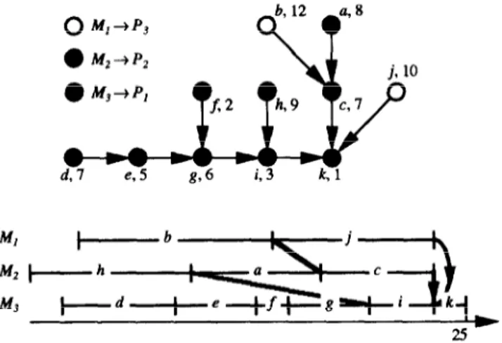
Figure 1 The assembly tree.

based on two main inputs (operations to be performed and machines available), two main sets of constraints (layout and flow management constraints) and a main goal (throughput maximization). Decisions can be conveniently introduced by imposing 7~ = {S,, SZ, . . . S,} to be a connected or a non connected partition. It is useful to note that if partition into connected components is allowed, the following results are obtained:

l if G is a tree, than the number of part transfers is minimized and, it is equal to m - 1;

l machine set-up is simplified.

A numerical example

Let us introduce the assembly tree G(N, A) in Figure 1. The 11 operations a, b, . . . , k (with the relative processing times) must be performed on three identical machines M,, M,, M3 which can perform all the operations. The transportation network E(P, C) is depicted in Figure 2.

A solution minimizing makespan is the one shown

in Figure 3 (solution 1). Here we have 7~ = {{c,d,

Figure 2 The transportation network.

0 M,+P,

e2 v”

i_.; kl 0 Ml-+P3

::‘:

d.7 e,5 g,6 i.3 k,l Figure 4 Solution 2. 2.5

h,k},{a,e,j},{b,f,g,i}} (each subset of the partition 7~

is represented by a color). ,? assigns machine M, to position P,, for i = 1,2,3. Function p trivially associates to each arc (i, ~)EA the arc (n,, ~L,)EC (that in this case always exists). Function o is depicted in the Gantt chart in Figure 3. Part transfers are highlighted by gray bold lines. In this case the makespan and the cycle time are equal to 24, while the number of part transfers equals 7. It is easy to verify that all the solutions minimizing makespan require cycling of parts in the transportation network.

The case of a solution not requiring part cycling is depicted in Figure 4. In this case the makespan equals 25. The corresponding cycle time remains equal to 24, therefore it also remains optimum. The number of part transfers is equal to 4, better than in the previous case. Notice that, by increasing the makespan by 1 (from 24 to 25) and without modifying the throughput, we can reduce the number of part transfers to 4 (solution 2).

In Figure 5 an assignment minimizing the number

of part transfers is depicted (solution 3). In this case the cycle time increases to 27, makespan is 28, whereas the number of part transfers is lowered to 2.

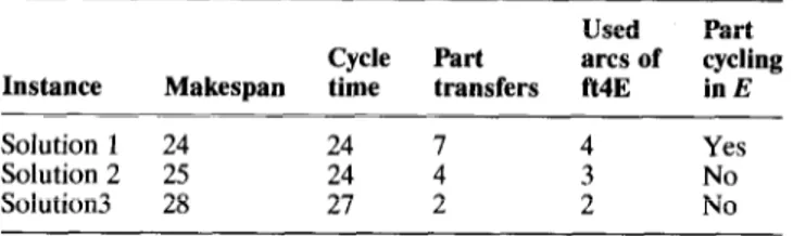
In Table 1 the numerical results for the above

example are summarized.

As shown in Table 1 the solution minimizing only one performance index (solution 1 minimizes

0 M1+P3

at”

l2

_9"'"

:::‘r;

e, 5 g. 6 i, 3 k, 1

Figure 5 Solution 3. Figure 3 Solution 1.

(4)

18 Modeling an assembly line for confguraion and flow management: A4 Lucertini et al.

Table 1 Performance of different solutions

Used Part Cycle Part arcs of cycling Instance Makespan time transfers ft4E in E

Solution 1 24 24 4 Yes

Solution 2 25 24 : 3 No

Solution3 28 27 2 2 No

makespan, solution 3 minimizes part transfer number) are not efficient with respect to the other, in particular, solution 1 leads to the necessity for part cycling in the transportation network, i.e. it may cause congestion in the transportation network. Nevertheless the solution minimizing traffic problems (solution 3) is not efficient with respect to the production rate. From an overall point of view a better solution is solution 2, which is a compromise among all the different performance indices.

General problem

Hereafter, a general statement of the problem (in the following referred to as GP) is given:

Given: G(N, A), E(P, C); Find: TC, II, p, o;

Such that:

1. the solution is feasible

2. a suitable mix of the following quantities is minimized:

(a) cycle time (b) completion time (c) number of part transfers By feasible solution we mean:

1. All the single decisions are individually feasible with respect to the initial constraints, i.e. each operation is assigned to a compatible machine and each machine is assigned to a compatible position, routing and sequencing do not violate the precedence relations expressed by the graphs E(P,C) and G(N, A) respectively.

2. The global solution is feasible, i.e. the single decisions are compatible with each other.

Clearly, the minimization of the cycle time corresponds to the maximization of the production rate of the plant. This is often equivalent to the minimization of the bottleneck machine workload. Nevertheless it is often verified in practice that it is the case that many different solutions exist, producing approxima- tely the same cycle time. In this case, other goals can be taken into account, such as the makespan or the part transfers minimization.

The minimization of the number of part transfers has currently received little attention in literature. In fact, this objective is not significant if transportation and set-up times are small with respect to the processing times. This is the case when a transportation network does not introduce delays due to the

traffic congestion problems (i.e. the number of part transfers is small and flows are ‘well structured’). On the other hand, in the case of complex material flow patterns, it is often possible to bound a priori the number of part transfers by looking for connected partitions, although this is not always feasible. In these cases part transfer minimization becomes significant (see “,“).

GP generalizes a wide set of decision problems at different levels of aggregation and with different time-spans. In practice, the conditions allowing for a solution of the whole problem are seldom verified. In a hierarchical approach some subproblems of GP are usually solved, where only a subset of decision variables are considered, while the others are either fixed or considered at a lower hierarchical level in the next stage of the solution procedure.

Let us distinguish three basic cases.

The first case is when rc is the only decision to be taken, while A is given and (p, o) are considered a

postetioti. This corresponds to the case of a given

flexible plant able to produce different types of products, typically within given families.The problem consists of assigning operations to existing machines.

The second case is when L is the only decision to be taken, while rr is given and (p, w) are considered a

post&on’. This corresponds to the case of the design

of a plant with dedicated machines, typically for large product rates of a small set of products. In this case the infrastructure to support the production (and often the transportation subsystem) are given and the problem is to assign clusters of operations, corresponding to existing machines to given positions of the plant.

The third case is when (p, o) are the only decisions to be taken, while (71, 2) are given. This corresponds to the well known scheduling problems. Depending on rc and ,J we can obtain job-shop, flow-shop or more general problems. In later sections we will deal with the first two cases.

Feasibility properties

In this section we discuss some important questions concerning the existence of a feasible solution of GP, the evaluation of its performances and, in general, the relationships between a certain decision and the performances of the resulting solutions.

In the following we will show that the first problem can be decomposed by operating separately on a subset of the decision variables rr, A, p, o rather than on the overall problem. Next we will show how these problems can be approached by representing the decisions rr, 1, p, w by suitably modifying the assembly graph G(N, A), i.e. by adding precedence constraints and dummy operations. In fact, any time a decision is taken, a new set of constraints is added to the problem data. On the resulting graph it is possible to easily evaluate performance indices such as the completion time, the cycle time and the part transfer number.

(5)

Modeling an assembly line for configuraion and flow management: M Lucertini et al. 19

More precisely, given z and 3,

l The routing decision p can be taken into account as denoted in the following: a routing is feasible if and only if:

V(i, j) E A either EL,

= 3>, or 3 a path on E from 1; to 1, _(I) Let us call intermediate machines all the machines of the sequence (if any) which are different from pi and a. We can distinguish three cases:

1. No path exists from 2, to &, in this case there is no feasible part transfer; we can represent this fact by adding to the graph G(N, A) the following set of arcs:

L = ( j, i): 3 a path on G from i to j,

lp a path on E from 1; to A,. ₍₂₎ As a consequence of the definition of L, condition (1) is equivalent to the condition L = 0.

2. If I, = 5, then no part transfer is needed and the sequence is still void.

3. If &#A, and there is a path from li to Jj, then a shortest path between the two machines is chosen: in particular if there is a directed connection then the sequence is formed by the two end-point machines only. If the sequence contains more than two machines, we must introduce a new set of k(i,j) dummy operations with zero processing time assigned to each intermediate machine. If we denote with x:,, x:,, . . . tici.” _1._I the dummy operations associated to the arc

(i,j), it is possible to build a new operation

graph from G(N, A), by denoting with N’ and A’ the new sets of nodes and arcs respectively:

N’= (NLJxl;,l <h<k(i, j) EA} ₍₃₎

A’ = (,;A i (y;;),@ X2 _)

k(i, j) = O ‘I’ ‘, , . . ., (XT’./), j) k(i,j) #O i

(4)

A new partition Z’ = {S,, S2, . . . . SL} is now introduced, due to the dummy operations introduced by p. It is clear that S: is the union of S, and the set of dummy operations assigned by p to the machine i.

l The sequencing decision w introduces a set 0 of precedence constraints between operations assigned to the same machine. These constraints simply correspond to add new arcs to the graph in such a way that m different linear orderings (one for each machine) are produced, i.e. for each pair

(i, j) of operations assigned to the same machine,

including dummy operations introduced in (3), either i precedes j or vice versa. Notice that not all the sequences lead to a feasible solution.

Eventually, let us denote with feasibility graph G’(N’,D) the graph where N’ is the new set of nodes,

introduced in (3), and D =A’ULUO. Let us consider any arc (i, j) ED. We associate to this arc a weight equal to the transfer time from i,, to 1,. Of course, in the case of iii = ,?, the arc weight will be equal to zero. It is straightforward to verify the following:

Remark 3.1. Any given solution (71, R, p, o) is feasible for GP ifund only if G’(N’, D) is acyclic.

Moreover, the different objective functions introduced in the general problem can be easily computed on the feasibility graph G’. In fact:

Part transfer number is given by the sum of the arcs cut by the partition 7~’ in the graph G’(N’, A’).

Completion time is given by the longest path (given as the sum of node and arc weights) on the graph G’.

The cycle time equals the longest path between two nodes assigned to the same machine.

Note that if G’ contains cycles the longest path is co. A necessary and sufficient condition for G’ to be acyclic, and thus for a solution to be acyclic is given in the following theorem.

Theorem 3.2. Given any acyclic graph G(N A), for any n E II, I& E A then there exist p, o such that

G’(N’, D) is acyclic if and only if the condition (1) is verified.

Proof. Necessity is trivial. In fact, by construction,

G’ acyclic implies L = 0 which is in turn equivalent to condition (1).

As sufficiency is concerned, we shall prove that if 71 E II, A E A and the condition (1) is satisfied then it is possible to find p and o such that G’ is acyclic.

Let G”(N’, A’) denote the graph obtained from G, after the decisions 7c and 1. If condition (1) is satisfied for each arc (i, j) EA, either 1, = iY or there is a path from A, to I7 in E. Therefore there is always a routing

p such that G” is acyclic.

Consider now a topological order on G”(N’, A’)

(this always exists, since G” is acyclic) and number accordingly the nodes. For each pair (i, j) of nodes of N’, such that i<j, there is no path from j to i. A feasible w can be simply obtained by sequencing the operations of N’ assigned to the same machine, respecting the topological order. This choice cannot

induce cycles in G’. 0

Remark 3.3. As feasibility is concerned, we are allowed to ignore the decisions p, o, in fact, proof of Theorem 3.2 suggests an algorithm to easily find such decisions, given rc and 1 satisfying condition (1).

Remark 3.3 allows us to focus our attention on the decisions 1. and 71, in particular, we are introducing the following two problems:

l

Given x E II, find /I E A such that condition (1) holds. We denote this problem by FP,.

Given 1, E A, find 7~ E n such that condition (1) holds. We denote this problem by FP, Since 1 is given, machines are fixed in certain positions so that problem FP;. consists in finding an assignment of operations to machines in such a way that

(6)

20 Modeling an assemb& line for configzuaion and flow management: M Lucertini et al.

operations are compatible with the machines they are assigned to and condition (1) holds.

Feasibility given 1

If G is a tree, by far the most usual situation, FP, can be solved in polynomial time with the algorithm FPOP (FP assignment of Operations to Positions)

sketched in the Figure 6. We denote by r the root of G. Quantity a(i, k) will be equal to 1 [0] if there is [not] a feasible solution in the subtree of G rooted in

i with the condition that operation i is assigned to machine k. Let M, denote the set of machines able to perform operation i, and P,, i EN, the set of predecessors of i. It is easy to find a feasible assignment of operations to positions, once a(i, k) are known for each i EN, k EM by a backward visit of the graph G.

Theorem 3.4. If G(N, A) is a tree, then FPOP either

finds a solution of FP, or prove infeasibility in 0(m2n) time units.

Proof, We will prove the theorem by induction on

the depth of the tree. We state by inductive hypothesis that FPOP applies for a tree with depth lesser or equal to k (the depth of a directed tree is the cardinality of its longest path in terms of number of arcs) and then we will show how FPOP holds for another tree with depth equal to (k + 1). It is easy to verify that FPOP applies when k = 0. We know by Theorem 3.2 that there is a feasible solution if and only if rc E n and condition (1) holds. Thus a(i, k) = 1 if and only if k EM, and for each (j, i) EA, there exists h EM such that a(j, h) = 1 and there exists the path from h to k in E.

If we consider a (k+ 1)-deep tree, the procedure FPOP applies for all the subtrees rooted in j, where j E P,. Suppose there is a feasible solution for each of

these subtrees: we can write a(r, k) = 1 if and only if

k E Mi and (1) holds for each (j, r) EA. The last one is

the condition expressed by FPOP, thus valid also for

(k + 1)-depth tree.

Step (a) of the procedure requires 0( [PiI x m xm)

time. Therefore the total cost is: C;!,lP,l xm xm

i.e. O(m*n). The proposition follows.

(7)

It is easy to show - following the proof - that, ,pf

E contains a spanning path, i.e. a directed path that contains all the nodes, the complexity of FPOP could be reduced to O(n’).

Feasibility given 7~

We are now giving some complexity results on FP,. In this section we restrict ourselves to the case of each machine compatible with each position. Given rr E II, x = {Sl, . ..) S,J it is possible to define a transporta-

tion graph T(M, R), where R = {(h, k):(i,j) EA, i ES,,

j E $1.

Theorem 3.5. FP, is NP-complete even in the case of

T(M, R) and E(e C) both trees, and if every machine is compatible with every position.

Proof. In order to prove the NP-completeness of

FP, we make use of the following NP-complete

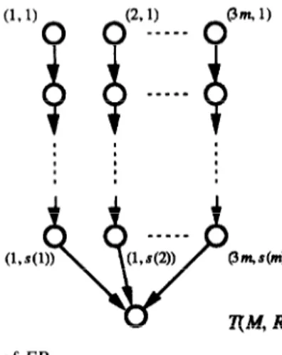
problem. 3-PARTITIONING (3P): Given a set A of

3m elements, a bound B E Z+ and a size s(a) E Z+ for each a EA such that B/4 <s(a) <B/2 and such that

znEAs(a) = mB, can A be partitioned into m disjoint

setsA,,A,, . . . . A, such that, for 1 <i I m, XasAis(a) = B (note that each A, must therefore contain exactly

three elements from A)? This problem is

NP-complete in the strong sense13. The strong NP-completeness implies the existence of a polynomial function p such that the problem 3P, restricted to only those instances i that satisfy MaxM %@-engthKl), is still NP-complete (see l3 for Procedure FPOP

Input: Assembly tree G(iV, A), set of compatible machines Mi for each operation i, A: pition of each machine in E.

Output: A feasible assignment, if any, Xi for each operation i. 1. For each leaf i E IV, let:

a&h) := 1 ifhcMi;

0 otherwise. (5)

2. Repeat the following until the root T is the only node left in Gz

(a) Consider any node i such that all its predecessors are leaves of G. Then for each k E M let:

a&k) := 1 if(kEMi)and@jEP?, 3h:o(j,h)=land~3thfromhtoIcinE);

0 otherwise.

(6) (b) Delete from G all the predecessors of node i.

3. FPA has a solution if and only if 3h E M, such that a(h,r) = 1.

(7)

Modeling an assembly line for conjiguraion and flow management: M Lucertini et al. 21

the proofs and the definitions of Max[l] and Length[q). The problem FP, is as follows: FP,: Given K E II, find 3, E A such that condition (1) is satisfied. Instance of FP, as follows: let T(M,R) and E(P,C) be both rooted trees. A rooted tree is a tree in which, for each subtree, the root is a successor of every node of the subtree. In particular, we consider the special case in which the rooted tree T(M, R) [E(P, C)] is composed by the root connected with 3m [m] chains. For each instance of 3P let us define an instance of

FP, by associating to each a EA a chain of T(M,R), composed by s(a) nodes, while each chain of E is composed by B nodes, as shown in Figure 7.

It is straightforward to observe that any instance of 3P is a yes-instance if and only if the corresponding instance of FP, is a yes-instance. Moreover, the reduction is polynomial since we can limit ourselves to the case of Max[l]~p(Length[q). Therefore FP, is NP-complete. It is also straightforward to verify that

FP, is not a number problem (see [GJ79] for the definition of number problem), therefore FP, is

NP-complete in the strong sense. 0

It is useful to consider the condensation of the graphs T(M,R) and E(P, C) as defined in 14. We say

strong component of a graph is any maximal strongly

connected subgraph. Let C,, Cz, . . ., C,, be the strong components of a graph G(N, A). The condensation of G(N, A) is a graph G*(N*, A*) having the strong components of G as its nodes, and an arc from C, to C, exists whenever there is at least an arc from a node of C, to a node of C, (see Figure 8).

Of course a condensed graph is always acyclic. Moreover the nodes are given weights equal to the cardinality IC, 1 of the corresponding strong component. In particular we denote by v(i), i E M* and w(j), j E P* the node weights in the graphs T*(M*, R*) and

E*(P*,C*), respectively. Obviously the following

equalities hold:

C!‘!;‘v(i) = CyYiw(j) = m. ₍₈₎

As a straightforward consequence of the definition above, a necessary condition for the existence of a solution of FP, is the following one.

Remark 3.6. A solution

qf

FP, exists onb if IM”I 2 IP*l.

A simple ‘fill-up’ heuristic for FP, is illustrated in

Figure 9.

Clearly, if this heuristic is repeated for all the possible topological orders of both T*(M*, R*) and

E*(P*,C*), then we are guaranteed to find a feasible

solution, if it exists. Nonetheless, in some cases we are guaranteed to find a feasible solution by applying the heuristic to only one order. In fact, if both

T*(M*, R*) and E*(P*,C*) contain a spanning path,

then there exists only one topological order for each graph, and we are done. Moreover, when E” contains a spanning path, and v(i) = 1 for each i EM* then, it is easy to see that, for any topological order induced

by T*, the fill-up heuristic finds a solution of FP,, or

proves infeasibility.

On the other hand, if the condition v(i) = 1 for each i E M* does not hold, the problem falls in the class of NP-complete problems, as shown below.

Theorem 3.7. FP, is NP-complete, even in the case of T* tree, E* path and each machine compatible with each position.

Proof We will reduce 3-PARTITIONING to our

problem. Given any instance of 3P, such that B is bounded by a polynomial function in m, we can associate the following instance of FP,: let T*(M, R)

be a star with 3m leaves, for each a EA we associate a leave of T* with weight s(a). Let E*(P,C) be a path with m nodes, each of weight B. Clearly a solution of 3P exists if and only if the corresponding solution of

FP, exists. Let us remark that the number of nodes n of the original graph T equals 3mB, therefore the reduction is polynomial. This completes the proof. n

Optimization properties

In this section, we deal with the problem of finding one or more optimal decisions for some polynomial cases of (GP), being a fixed subset of the decision variables.

In particular we consider the problem (GP) in the case of G tree, E containing a spanning path, each

(8)

22 Modeling an assembly line for con$&uraion and flow management: M Lucertini et al.

Figure 8 A graph and its condensation.

machine compatible with each position, and given 7r= {S,, . ..) S,} connected, as defined in the second section. In this case it is possible to find in polynomial time a solution o*,Iz*,p* such that the completion time, i.e. the time necessary to complete all the operations, is minimized.

Since 7c is connected, each subgraph of G induced byS,,,h=l,..., m is a tree. Therefore for each h = 1, . . ., m there is a node r(&), root of the subtree induced by S,. If there is a directed path from a node j E S, to a node i E Sk, k#h, then Y(&) belongs to this

path. Hence, the completion time C,, of operation y(,S,,), for each h = 1, . . ., m, corresponds to the completion time of all the operations assigned to machine h. Let us introduce a release date 5 for each node j of the subgraph:

rj = 0 if j has no predecessors

~rj 2 ri+Pi if j is preceded by i E N’

rj 2 C, if j is the successor of machine k ₍₉₎

Here pi denotes the processing time of operation i.

Notice that, as soon as the operations assigned to a machine are scheduled, the release dates will change according to (4), because new arcs are added to the set A’. Since dummy operations must be scheduled they will affect the completion time. A lower bound for the values of release dates and completion times can be found in the hypothesis, that no dummy

operation exists or they do not affect the system behaviour.

As we are restricting our attention to the case of E(P,C) containing a spanning path, we will deal with two main different scenarios. In the first case we consider a complete acyclic digraph E(P,C). In the second case we are concerned with a line, i.e. a digraph E(P, C) where C = {(h, h+ l), h = 1, . . . ,

lq - 11.

We will show that any intermediate situation can be viewed within these two scenarios.

We suppose the nodes of E are numbered according to the (only) topological order, then C = {(i, j): i <j}.

Case 1: E is a complete acyclic graph. In this case

the problem of minimizing the makespan is trivial: any feasible assignment 1 (see theorem on feasibility 3.2) is optimal. The decision p* simply consists of assigning no dummy operations; in fact for each pair of position h, k, either there is a directed connection or there is no path connecting them. Once il has been decided, the remaining problem is to schedule operations with given release dates, on one machine, in order to minimize completion times, so that LO* is given by processing first the operations with earliest release dates (ERD rule). The procedure R-dates (described in Figure 10) finds co* together with the smallest release dates for each operation i EN and completion times for each machine, which satisfy eqn (4). Eventually, the values of completion times will be equal to the release dates of their successors. Of course, the makespan is equal to max {C,, . . . , CJ.

Case 2: E is a line. Also in this case we can achieve the same value of makespan, as shown in Theorem 4.1. In fact, the simple dynamic programming procedure MIN_MAKESPAN described in Figure 11,

assigns machines to positions in such a way that dummy operations do not affect the overall makespan, i.e. each dummy operation always finds a machine available.

Clearly the makespan obtained in Case 1 is a lower bound of the optimal solution for any graph E, since there are no dummy operations to be scheduled.

Procedure Fill-Up

Input: Wheighted graphs T*(M’, R*) and E’(P*, C’).

Output: A solution of FP,.

1. Assign an index to each node of T*(M*, R*) and E*(P) C’) equal to its position in a top logical order (therefore the node in the last position has the maximum index).

2. Repeat the following until either a solution is found or not:

(a) Chocee the node i of T’ (M*, R’) , not yet assigned, with maximum index and the node j of E* (P’ , C’), with maximum index and weight strictly greater than zero.

(b) If w(i) > w(j) th en no solution is found, else the node i is assigned to position j and: w(j) := w(j) -v(i).

(9)

Modeling an assembly line for configuraion and flow management: M Lucertini et al. 23

Procedure Mates

Input: assembly tree G(N, A) with operations processing times, connected partition 7r and corresponding graph T(M, R) .

Output: decision w, values of minimum completion times Ch, for each subset of operations Sh (h = 1 ,.**, m).

1. Initialize release dates values: vi = 0 for each i E N. 2. Let L = {current leaves of T}.

3. If L is empty STOP.

4. For each h E L do the following:

(a) Compute Ch by scheduling operations with an ERD rule (decision u.) (b) Let T, := C,,, where 2 E N is the successor of Sh.

5. Update T, by deleting all the current leaves: A4 := M \ L.

6. Go to 2. Figure 10 Procedure R-dates.

Theorem 4.1. If G(N, A) is a tree, E(E: C) contains a spanning path and x is given and connected, then the problem of finding a solution(w*, A*, p*) minimizing

the makespan, is polynomial.

Proof. If E is a line, the procedures R-DATES and

MIN_MAKESPAN find a makespan equal to the lower bound obtained in the case of E complete acyclic graph. Therefore the solution is optimal. In any other case, we can obtain the same makespan. As regards the complexity of the procedures, it is easy to compute it in 0(n2) both for R-DATES and

MIN_MAKESPAN. This completes the proof. 0

Remark 4.2. Theorem 4.1 shows that makespan cannot be reduced by simply adding arcs to the spanning path.

If we minimize cycle time, we have a different complexity for the case of connected partition and the case of general partition 7~. It is easy to verify that, if 7~ is connected, then the cycle time minimization can be achieved by looking for a partition z minimizing the workload of the busiest machine. For

this purpose there exist efficient (polynomial) algorithms finding such a partition on paths and trees’5x’6.

Furthermore, the problem of scheduling IZ jobs on one machine, with given release dates, acyclic precedence constraints, to find the minimum completion time, is polynomial”.

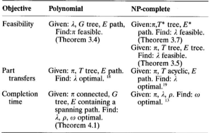
Table 2 summarizes the complexity results

concerning the optimization problem when E is a line.

Conclusions

The paper outlines and analyzes a unified framework for designing (or re-designing) the configuration of a given production plant and the corresponding network of material flows. The integrated approach could produce substantial advantages in many practical cases. However, the decision model falls into the format of a large scale integer programming model, often too difficult to solve for real size appli-

Procedure Minslakespan

Input: graphs T(M,R) (tree) and E(P,C) (line), values Ch of completion times for each subset of operations assigned to a machine h E M. (IA41 = IPI.)

Output: feasible assignment A’ minimizing makespan.

1. Assign the root T of T to the last position of the line: A*(T) := m.

2. Sort the l&l predecesso rs of the root in increasing order of completion time (C1 5 Cz 5 . . . 5 CIi%O.

3. For each h E P, perform Minmakespan for the subtree of T rooted in h (call it STh) on the part of the line E from position 2 + c:it ISTil to position 1 + & IST’il.

(10)

24 Modeling an assembly line for conjiguraion and flow management: M Lucertini et al.

Table 2 Complexity results

Objective Polynomial NP-complete

Feasibility Given: 1, G tree, E path, Find:rr feasible. (Theorem 3.4)

Part Given: rr, T tree, E path. transfers Find: 1 optimal. ” Completion Given: n connected, G

time tree, E containing a spanning path. Find: 1, p, 0 optimal. (Theorem 4.1)

Given:x,T* tree, E* path. Find: 3, feasible. (Theorem 3.7) Given: rr, T tree, E tree.

Find: 1 feasible. (Theorem 3.5) Given: rr, T acyclic, E path. Find: 1, optimal.” Given: R, d, p. Find: o optimal. ”

cations. In such cases it is possible to follow a greedy- like approach and to determine a value of the decision variables applying a sequence of different criteria. In a first step, we will find the value of rc or J on the ground of practical considerations. n can sometimes be obtained in the process-plant integrated design phase by clustering operations on a set of good existing machines. A can be sometimes obtained in the machine layout phase on the ground of machine-positions feasibility constraints. In a second step, we can solve one of the decision modules presented in the paper finding either 2 or rc (models FP, or FP, respectively). Finally, in a third step, we can find the scheduling (w, A) by some simple heuristic, in the way most managers do, or by some more sophisticated methods. This mix of practical considerations, optimization technique for configuration and flow management scheduling techniques, has been proved to be effective in many practical cases.

In the large production case, typical of car components and electronic units productions, most of the operations are assigned to dedicated machines in the design phase and only few handling operations can be done in different ways by different machines. Moreover, the strong precedence constraints among operations, introduce corresponding constraints among machine and positions.

In the FMS case, incomplete flexible machines (machines without tools) are already in position. In this case the problem of assigning machines to positions is in reality an assignment of tools to positions, generally with only a few feasible assignments. The operations to machines assignment problem is, in this case, the critical point of the production strategy. As we can see by those

examples, most of the real problems do not fall completely into the FP, or FP, format, but a wide set of decision variables do. The unified model helps in finding the right way to approach those mixed problems, and enlightens the modeling solution problems.

A next stage in the research work will be devoted to the analysis of relevant applications in order to verify the benefits of this systematic framework to approach decision problems up to now solved on the ground of ‘practical considerations’.

References

Askin RG and Standridge CR Modeling and analysis of manufacturing systems. John Wiley and Sons, New York, 1993. Helgeson WB, Salveson ME and Smith WW ‘How to balance an assemblv line’, Management Report no. Z New Caraan, Carr Press, Division for Advanced Manaiement, 1654.

Gutjahr, A. and Nemhauser, GL ‘An algorithm for the line balancing moblem’. Management Science Vol 11 No 2 (1964) 308-315- -

Baybars, I ‘A survey of exact algorithms for the simple assemblv line balancing oroblem’. Management Science Vol 32 (1986) 909-932 - 1 ’ ”

Ghosh, S and Gagnon, RJ ‘A comprehensive literature review and analysis of the design, balancing and scheduling of assembly systems’, International Journal of Production Research Vo127 No 4 (1989) 637-670

Chase, RB ‘Survey of paced assembly lines’, Industrial Engineering Vol 6 (1974)

Johnson, RV ‘Optimally balancing large assembly lines with FABLE’, Management Science Vo134 No 2 (1988) 240-253 Monden Y. Toyota production system. Norcross, GAIndustrial Engineering and Management Press.

Agnetis A, Lucertini M, Nicoletti S, Nicol’o F, Oriolo G, Pacciarelli D, Pacifici A, Pesaro E and Rossi F ‘Scheduling flexible flow lines in an automobile assembly plant’, European Journal of Operational Research Vol 97 (1997) 348-362. 10 Berrada, M and Stecke, KE ‘A branch and bound approach for

workstations load balancing in flexible manufacturing systems’, Management Science Vo132 (1986) 1316-1335

11 Lucertini M, Pacciarelli D and Pacifici A ‘Layouts in assembly problems’, Proceedings of the 1994 Japan-USA. Symposium on Flexible Automation, Kobe (Japan), 11-18 Jury 1994.

12 Lucertini, M, Pacciareili, D and Pacifici, A ‘Optimal flow management inflexible assembly systems: the minimal part transfer problem’, Systems Science Vo122 No 2 (1996) 69-80 13 Garey MR and Johnson DS. Commuters and intractability.

Freeman, 1979.

14 Harary F Graph theory. Addison-Wesley, Reading, 1969. 15 Becker, RI, Per-l, Y and Schach. SR ‘A shifting aleorithm for

min-max tree partitioning’, J.A.C.M. Vo129 (19y82) 58-67 16 Becker, RI and Perl, Y ‘A shifting algorithm for tree parti-

tioning with general weighting functions’, Journal of Algotithms vo14 (1983) 101-120

17 Lawler, EL ‘Optimal sequencing of a single machine subject to ~~_\~rce constraints’, Management Science Vol 19 (1973) 18 Adolphson, RC and Hu, A ‘Optimal linear ordering’, SIAM

Journal ofApplied Mathematics Vo125 No 3 (1973) 403-423 19 Even S and khiloach Y ‘NP-completeness of several arrange-

ment problems’, Report n. 43, Haifa, Israel: Dept of Computer Science, 1975.