Accepted Manuscript
Estimation of bathymetry (and discharge) in natural river cross-sections by using an entropy approach
G. Farina, S. Alvisi, M. Franchini, G. Corato, T. Moramarco
PII: S0022-1694(15)00296-6
DOI: http://dx.doi.org/10.1016/j.jhydrol.2015.04.037
Reference: HYDROL 20396
To appear in: Journal of Hydrology Received Date: 17 November 2014 Revised Date: 13 April 2015 Accepted Date: 18 April 2015
Please cite this article as: Farina, G., Alvisi, S., Franchini, M., Corato, G., Moramarco, T., Estimation of bathymetry (and discharge) in natural river cross-sections by using an entropy approach, Journal of Hydrology (2015), doi: http://dx.doi.org/10.1016/j.jhydrol.2015.04.037
This is a PDF file of an unedited manuscript that has been accepted for publication. As a service to our customers we are providing this early version of the manuscript. The manuscript will undergo copyediting, typesetting, and review of the resulting proof before it is published in its final form. Please note that during the production process errors may be discovered which could affect the content, and all legal disclaimers that apply to the journal pertain.
1 Estimation of bathymetry (and discharge)
1
in natural river cross-sections by using an entropy approach 2
3 4
G. Farina(1), S. Alvisi(1)*, M. Franchini(1), G. Corato(2), T. Moramarco(3) 5
(1)
Engineering Department, University of Ferrara, via Saragat, 1, 44121 Ferrara, Italy 6
(2)
Département Environnement et Agro-biotechnologies, Centre de Recherche Public Gabriel 7
Lippmann, 41 Rue du Brill, 4422 Belvaux, Luxembourg 8
(3)
Research Institute for Geo-Hydrological Protection, National Research Council, Via Madonna 9
Alta,126, 06128 Perugia, Italy 10
11
*Corresponding author: [email protected]; tel: +39 0532974849; fax: +39 0532974870 12
13
Abstract 14
This paper presents a new method for reconstructing the bathymetric profile of a cross section based 15
on the application of the principle of maximum entropy and proposes a procedure for its 16
parameterization. The method can be used to characterize the bathymetry of a cross-section based 17
on a reduced amount of data exclusively of a geometric type, namely, the elevation of the lowest 18
point of the channel cross-section, the observed, georeferenced flow widths and the corresponding 19
water levels measured during the events. 20
The procedure was parameterized and applied on two actual river cross-sections characterized by 21
different shapes and sizes. In both cases the procedure enabled us to describe the real bathymetry of 22
the cross-sections with reasonable precision and to obtain an accurate estimate of the flow areas. 23
With reference to the same two cases, we show, finally, that combining the bathymetry 24
reconstruction method proposed here and an entropy-based approach for estimating the cross-25
sectional mean velocity previously proposed (Farina et al., 2014) enables a good estimate of 26
discharge. 27
28
Key-words: bathymetry, entropy, streamflow measurements, remote sensing 29
2 1. Introduction
31
The discharge of a river, quantifiable by multiplying the mean stream velocity by the flow area of 32
the cross-section, represents a fundamental parameter for water resource management, flood control 33
and land protection. 34
In common practice, discharge is generally estimated using the velocity-area technique, in which 35
the cross-section area is discretized into an adequate number of segments, each delimited by two 36
verticals. The discharge associated with each segment is determined as the product of the segment 37
surface area and the corresponding mean velocity, the latter being obtained by means of direct 38
current-meter measurements in points within (on an axis) or on the perimeter of the segment itself; 39
finally, the total discharge is calculated as the sum of the discharges of the individual segments. 40
This procedure for estimating discharge thus entails sampling the stream velocity in points located 41
at different depths along a sufficient number of verticals distributed within the flow area; these 42
verticals are generally spaced in such a way as to provide an adequate representation of the 43
variations in velocity across the cross-section. 44
At the same time, the cross-section profile is schematically represented by connecting the bottom 45
points of the different verticals so that the flow area is the area between the cross-section profile and 46
the free surface of the stream. 47
Although this technique proves to be particularly accurate, it is not easy to implement, as it relies on 48
measurements of an episodic type that are difficult to automate, take a considerable amount of time 49
and are not very accurate in proximity to the river bed due to the presence of vegetation; moreover, 50
the strong currents that typically occur during exceptional flood events may expose operators to 51
hazards or even make it impossible to take proper flow velocity measurements. 52
Acoustic Doppler Current Profiler (ADCP) can represent an alternative, since it provides the spatial 53
distribution of velocity, but it is costly because of all the operations tied to post-processing and data 54
filtering. 55
3 Another valid alternative for estimating discharge is provided by the entropy method, which, based 56
on the principle of entropy maximization (Jaynes, 1957), was applied by Chiu (1987, 1988) to 57
reconstruct the (probability) distribution of velocity in a channel cross-section. Chiu was able to 58
identify a linear relationship, which is the function of a parameter - M - between the mean velocity 59
Ū and the maximum velocity umax of a river cross-section (Chiu, 1988; Chiu, 1991; Xia, 1997), i.e., 60
u M
f
U max, .
61
In practical terms, starting from a single measurement of the cross-sectional maximum velocity umax 62
- easily determinable as it generally manifests itself in the upper-middle portion of the flow area 63
(Chiu,1991; Chin and Murray, 1992; Chiu and Said 1995; Moramarco et al., 2004), which remains 64
easily accessible for sampling even during substantial flooding - it is possible to arrive at an 65
estimate of the mean velocity Ū and then, by multiplying the latter by the flow area of the cross-66
section, at an estimate of the discharge. 67
However, the parameter M must first be estimated in order to convert the maximum observed 68
velocity umax into the cross-sectional mean velocity Ū; this dimensionless parameter does not vary 69
with the velocity (or discharge) and represents a typical constant of a generic cross-section of a 70
channel/river (Xia, 1997; Moramarco et al., 2004). The parameter M is generally estimated by linear 71
regression performed on a substantial set of pairs of values umax-Ū, which are obtained by means of 72
the velocity-area method; hence, numerous current-meter measurements taken during multiple flood 73
events are required. Indeed, these latter are the same measurements typically required for building a 74
stage-discharge relationship. 75
However, some recently proposed procedures (Farina et al., 2014) enable the parameter M to be 76
estimated relying on a more limited set of velocity measurements; these range from current-meter 77
measurements across the entire flow area to one measurement of surface maximum velocity alone. 78
In short, once the parameter M has been estimated by means of these procedures, it will be possible, 79
4 as already stated, to estimate the mean velocity, and then multiplying the latter by the flow area of 80
the cross-section, to have an estimate of discharge. 81
However, it should be observed that in order to be able to estimate the discharge using the entropy-82
based approach just outlined, we need to know the geometry of the river cross-section for the 83
purpose first of estimating the parameter M and then of estimating discharge (quantification of the 84
flow area). The problem to be confronted, therefore, is to reconstruct the cross-section geometry. 85
In order to determine the cross-section geometry we can presently rely on various bathymetric 86
survey techniques, depending on the size of the cross-section we are investigating. The active bed 87
of non-navigable rivers (water less than 1 meter deep) can be surveyed simply by wading and taking 88
direct measurements of points at the gage site or using GPS measurements; if, during exceptional 89
flood events, the depth increases to such an extent that it is no longer possible to stand in the water, 90
it will be necessary to rely on an ultrasonic bathymeter or an ADCP connected to a GPS survey 91
system which can provide a precise, real-time survey of the course of the float it is mounted on 92
(Costa et al., 2000; Yorke & Oberg, 2002). In addition to providing a spatial distribution of 93
velocity, this technology makes it possible to have a high-definition map of the bed investigated, 94
but as previously observed it is both time-consuming and costly because of all the operations tied to 95
post-processing, data filtering, graphic rendering and inputting data to the databases. 96
Several authors have therefore sought to determine the bathymetric profile indirectly by analytic 97
means based on the measurement of surface velocity, as this parameter can be easily determined by 98
using latest-generation non-contact radar sensors (Costa et al., 2006; Fulton & Ostrowski, 2008). 99
The method developed by Lee et al. (2002) is based on the assumption of a logarithmic velocity 100
profile, but it requires knowledge of such hydraulic variables as the energy slope and Manning’s 101
roughness, which are very often not known. In a manner analogous to what Chiu (1987, 1988) did 102
for velocity, Moramarco et al. (2013) applied the principle of maximum entropy to estimate the 103
probability density function of water depth and the flow depth distribution along the cross-section, 104
5 assuming a priori that the cumulative probability distribution function increases monotonically with 105
the surface flow velocity. 106
In this paper we describe the theoretical development and practical application of a new analytical 107
method that is likewise derived from the principle of maximum entropy, but is able to dissociate the 108
bathymetry estimate from the surface velocity measurement. Using the proposed method, in fact, 109
we can describe the bathymetric profile of the cross-section investigated on the basis of a smaller 110
amount of information, exclusively of a geometric character, namely, the elevation of the lowest 111
point of the channel cross-section and the georeferenced flow width (i.e. a flow width whose end 112
coordinates are known) associated with a precise water level recorded during a sufficient number of 113
flood events. 114
Below we shall start off by presenting a summary overview of what is already known from the 115
literature concerning the entropy concept and the principle of maximum entropy, as they represent 116
the theoretical assumptions underlying this paper. We shall then illustrate the method for 117
reconstructing the bathymetry of a river cross-section and show how this method can be 118
parameterized for operational purposes. The proposed procedure is applied in two case studies, one 119
regarding the Ponte Nuovo gage site along the Tiber River in central Italy and the other the Mersch 120
gage site along the Alzette River in Luxembourg. Making reference to the same two sites, we then 121
show how the cross-sections thus reconstructed can be effectively used to estimate discharge by 122
combining (multiplying) the estimate of the flow area with the cross-sectional mean velocity as 123
determined using the entropy approach proposed by Chiu (1987,1988). We conclude the paper by 124
presenting some final considerations. 125
126
2. Entropy and the principle of maximum entropy (POME) 127
The entropy of a system was first defined by Boltzmann (1872) as “a measure of our degree of 128
ignorance as to its true state”. In his information theory, Shannon (1948) introduced what is today 129
6 called “entropy of information” or also Shannon entropy, defining it quantitatively in probabilistic 130
terms for a discrete system as: 131 132
j ln j j H X
p X p X (1) 133 134where p(Xj) represents the (a priori) probability mass function of a system being in the state Xj,
135
belonging to the set
Xj, j1, 2,...
. 136If the variable X is continuous, the entropy is expressed as: 137 138
ln
H X
p X p X (2) 139 140where p(X) now represents the probability density function. 141
The Principle of Maximum Entropy (Jaynes, 1957) affirms that, in the presence of data and/or 142
experimental evidence regarding a given physical phenomenon, for the purpose of estimating the 143
associated probability distribution it will be sufficient to choose a model that is consistent with the 144
available data and at the same time has the maximum entropy. 145
From a strictly mathematical viewpoint, the form of the probability density function p(X) which 146
maximizes the entropy H(X) defined by eq. (2) and subject to a number m of assigned constraints in 147 the form: 148 149
,
1, 2,... b i i a G
X p dX i m (3) 150 151can be obtained by solving the following equation: 152
7
1 ln , 0 m i i i p p X p p p
(4) 154 155where λi is the i-th Lagrange multiplier (Vapnyarskii, 2002).
156
The principle of maximum entropy was applied by Chiu (1987, 1989) to describe the two-dimensional
157
flow velocity distribution in a channel cross-section based on the cross-sectional maximum velocity umax
158
and the dimensionless parameter M, and by Moramarco et al. (2013) to estimate the probability density
159
function of water depth and the flow depth distribution along the cross-section, assuming a priori 160
that the cumulative probability distribution function increases monotonically with the surface flow 161
velocity. In a similar manner, below we outline a method for determining the geometry of a natural
162
channel that uses the entropy maximization principle, but is independent of the surface velocity
163
measurement.
164 165
3. Reconstruction of the bathymetry of a river cross-section 166
Let us consider a generic cross-section of a river with a free surface flow and let D be the maximum 167
depth in the cross-section; assuming a Cartesian reference system whose origin is fixed on the 168
surface at the top of the vertical where the depth is greatest, the coordinate y in Figure 1 represents 169
the depth and x the horizontal distance from the vertical where we have the maximum depth D; 170
moreover, let h be the water depth (relative to the surface), corresponding to a vertical at a 171
horizontal distance x from the reference vertical of the system. Finally, let us assume that the depth 172
h decreases monotonically along the transverse direction, going from the maximum value D at the 173
reference vertical (x=0) to 0 on the river bank x=L (see Figure 1). 174
175
Figure 1 approximate location 176
8 Assuming that the depth h represents a random variable, let F(h) be the corresponding cumulative 178
probability distribution function and p(h) the probability density function given by: 179 180 ( ) ( ) dF h p h dh (5) 181 182
In particular, the probability density function p(h) to be identified must satisfy the unity constraint: 183 184 0 ( ) 1 D p h dh
(6) 185 186where D is the maximum depth, i.e., the maximum value of h at the point in which x=0. 187
An additional constraint on the flow depth distribution is represented by the mean value Hm of the
188
depth h, which can be expressed as: 189 190 0 ( ) D m h p h dhH
(7) 191 192If the cross-section geometry is not known, nor will the corresponding probability density function 193
p(h) be known; however, it can be estimated by applying the principle of maximum entropy through 194
the constrained maximization of the entropy (see eq. (4) with 1 p h
and 2 h p h
):195 196
1 2 ( ) ln ( ) ( ) ( ) 0 p h p h p h h p h p p p (8) 197 198The solution of eq. (8) provides the expression of the probability density function: 199
9 200 1 1 2 ( ) h p h e e (9) 201 202
On the basis of eq. (9), eq. (5) becomes:: 203 204 1 1 2 ( ) h F h e e h (10) 205 206
which relates the depth h to the corresponding cumulative probability function F(h). 207
By substituting eq. (9) in the first constraint equation (6) and integrating and substituting the result 208
in eq. (10) and integrating, the following expression is obtained: 209 210
2
2 1 ( ) ln 1 D 1 ( ) h x e F h x (11) 211 212which gives us the depth h of a cross-section at a point corresponding to a vertical at a distance x 213
from the vertical where we have the maximum depth. This expression is clearly a function of the 214
cumulative probability distribution F(h) and, therefore, in order to be able to estimate the shape of 215
the cross-section it is necessary to formulate an expression with which to quantify F(h). 216
To this end, Moramarco et al. (2013) assume for the cumulative probability distribution function 217
F(h) an expression given by the ratio between the surface velocity us(x) and the maximum surface
218
velocity usmax. However, as also assumed in Moramarco et al. (2013), since the link existing
219
between the two variables x and h is monotonic, the probability that the depth h(x) will remain less 220
than or equal to a given value h* coincides with the probability that the x coordinate will be greater 221
than or equal to the corresponding x*: 222
10
*( *)
( *) ( *) 1 ( *) 1 * / F h x P hh P xx P xx x L (12) 224 225Therefore, eq. (11) can be rewritten as: 226 227
( ) Dln W W 1 x h x e e W L (13) 228 229where W
2D is a dimensionless parameter characteristic of the river cross-section. 230Eq. (13) thus enables us to describe the bathymetry pattern of a cross-section once the parameter W 231
is known. 232
Since at this point F(h), and thus p(h), are formally known, the solution of integral in eq. (7) 233
produces the following result: 234 235 1 ( ) 1 W m W e H D W D e W (14) 236 237
It is worth observing, incidentally, that the value of the parameter W varies from very small values 238
(close to zero) for triangular cross-sections (that is, where Hm/D0.5) up to very high values for
239
approximately rectangular cross-sections (that is, where Hm/D1). Theoretically, the parameter W
240
could thus be estimated by linear regression performed on a substantial set of pairs of values Hm-D
241
(Moramarco et al., 2013), but this approach would entail carrying out a bathymetric survey across 242
the entire river cross-section in order to quantify Hm.
243
In the paragraph below we describe a new procedure for estimating the dimensionless parameter W 244
that does not require any bathymetric survey to be conducted and is based only on a reduced 245
amount of information of an exclusively geometric type. 246
11 247
3.1 Estimate of the parameter W
248
Let us suppose that n (with n ≥ 2) flood events have occurred over time in the river cross-section 249
whose geometry we want to reconstruct and that observed, georeferenced flow width (i.e. whose 250
extremes have known coordinates) and water level data are available for every case. Let us consider 251
the flood event during which the maximum water level was observed and set the origin of the 252
Cartesian reference system on the free surface associated with that event, in the point of maximum 253
depth, implicitly assuming that the elevation of the deepest point of the cross-section is known. For 254
all practical purposes, the point of maximum depth (x=0) can be positioned in correspondence of 255
the vertical in which the maximum surface velocity is observed. 256
257
Figure 2 approximate location 258
259
Based on the available geometric data, and once the aforesaid reference system has been defined, it 260
will be possible to quantify (see Figure 2): 261
the maximum depth D, i.e., the largest distance between the river bed and the free surface of the 262
event; 263
the coordinates (ll,i, δi) and (lr,i, δi) of the extremes, respectively on the left and right banks, of 264
the flow width corresponding to each event, with the exception of the largest (i=1,2…n-1) 265
(given that δi represents the depth associated with the i-th water surface/flow width relative to 266
water surface/flow width associated with the largest/maximum flood event); 267
the distances Ll and Lr of the extremes of the flow width of the largest flood relative to the
268
vertical of the reference system, respectively on the left and right banks. 269
Eq. (13), which describes the variation in the depth h (calculated relative to the free surface of the 270
largest flood event) along the horizontal coordinate x, can thus be rewritten to the left and right of 271
the reference vertical by setting L=Ll and L=Lr, respectively:
12 273
( ) ln 1 0 ( ) ln 1 0 W W l l l l l W W r r r r r x D h x e e with x L W L x D h x e e with x L W L (15) 274 275In this manner we describe two functions, both constrained to passing through two fundamental 276
points, namely, the lowest point of the channel cross-section (xl= xr=0 , h=D) and the extreme
277
corresponding to the greatest flow width (xl=Ll, h=0 on the left and xr=Lr, h=0 right banks of the
278
river, respectively). The combination of these two functions delineates the bathymetric profile of 279
the entire cross-section, which, for given values of D, Ll and Lr, varies its shape with variations of
280
the parameter W. 281
Let xl,i and xr,i be the coordinates, respectively on the left and right banks, obtained by rearranging
282
eq. (15) and imposing h=δi (i=1,2…n-1); that is, xl,i and xr,i represent the coordinates of the
283
bathymetric profile described by eq. (15) at the depth associated with the flow widths of the n-1 284
events (see Figure 2) calculated starting from the flow width associated with the maximum event: 285 286
/ , / , 1, 2,.. 1 1 1, 2,.. 1 1 i i W D W l l i W W D W r r i W L x e e with i n e L x e e with i n e (16) 287 288It should be noted that a variation in the parameter W is reflected in the shape of the bathymetric 289
profile and, consequently, in the coordinates xl,i and xr,i. It is assumed, therefore, that the optimal
290
estimate of W is the one whereby the profile defined by eq. (15) best reproduces the entire cross-291
section, i.e., the value that minimizes the sum of horizontal deviations (in absolute value) between 292
13 the profile itself and the extremes of the flow widths of the n-1 events at an equal depth δi defined
293 as follows: 294 295 1 , , , , 1 (W) n l i l i r i r i i err l x l x
(17) 296 297 4. Case studies 298The proposed method for reconstructing bathymetry and estimating the parameter W was applied 299
and verified using data regarding the Ponte Nuovo gage site located along the Tiber River (Central 300
Italy) and the Mersch gage site located along the Alzette river (Luxembourg) (see Figure 3). 301
302
Figure 3 approximate location 303
304
The basin closed at Ponte Nuovo drains an area of around 4135 km² and is equipped/monitored with 305
a cableway that enables current-meter velocity measurements to be made at different depths and 306
depth measurements on different verticals. 307
The Mersch station subtends a more limited drainage area, about 707 km², and velocity 308
measurements are performed with an Acoustic Doppler Current Profiler. 309
Figure 3 shows a map of the two basins subtended by two river cross-sections concerned and their 310
positions, while Figure 4 shows the bathymetric survey data. In particular, for Ponte Nuovo section 311
the bathymetry shown in Figure 4 was obtained by a topographic survey done in 2005, whereas for 312
Mersch was obtained by elaboration of the ADCP measurements done during the most severe flood 313
event occurred in 2006. 314
315
Figure 4 approximate location 316
14 As can be seen from the figure, the sites under examination are characterized by cross-sections of 318
different size and shape; in particular, the Ponte Nuovo cross-section has a trapezoidal shape, while 319
the shape at the Mersch site more closely resembles a triangle. Topographic surveys and flow depth 320
measurements conducted at the sites over a number of years have shown no significant 321
modifications in geometry, which can thus be considered as unchanged over time. 322
The data set for the Ponte Nuovo site consists of n=9 flood events recorded from December 1999 to 323
April 2004, whereas data for the Mersch site consists of n=14 flood events recorded from December 324
2004 to July 2007. The main hydraulic characteristics of the events are provided in Table 1 and 325
Table 2 for the Ponte Nuovo and Mersch site respectively. For each event the discharge Q, the 326
maximum water depth D, the flow width Ltot=Ll+Lr, the flow area A and the ratio of the mean and
327
maximum water depth Hm/D are provided. In particular, the discharge Q was calculated on the basis
328
of point velocity measurements using a variant of the Mean-Section Method (UNI EN ISO 748, 329
2008). As can be observed the events considered are characterized by a broad range of discharge 330
values, between 6.70 and 427.46 m3/s for Ponte Nuovo and between 2.27 and 37.25 m3/s for 331
Mersch. Furthermore, it is worth noting that Ponte Nuovo is characterized by higher values of the 332
Hm/D ratio (0.8-0.9) than Mersch (0.62-0.7), in agreement with the trapezoidal and nearly triangular
333
shapes of the two cross-sections respectively, given that the ratio Hm/D varies from 0.5 for
334
triangular section up to 1 for rectangular section. 335
Based on numerous pairs of values of Hm-D, Moramarco et al. (2013) estimated by means of a least
336
squares linear regression W values equal to 6.6 and 2.2 for Ponte Nuovo and Mersch respectively. 337
These two values of W were taken as reference values with which to compare the corresponding 338
values furnished by the method for estimating the parameter W proposed here. 339
Below we present and discuss the results we obtained in our estimation of the parameter W, as well 340
as the reconstruction of the bathymetry for each of the two cross-sections considered. The results in 341
terms of the discharge estimates obtained by combining the flow areas estimated using the method 342
15 proposed here with the cross-sectional mean velocities estimated by applying the method proposed 343
by Farina et al. (2014) are also presented for both sites. 344
345
5. Analysis and discussion of results 346
5.1 Analysis and discussion of results of bathymetry reconstruction 347
For both cross-sections under examination, the bathymetry was reconstructed using eq.(13) after the 348
parameter W had been estimated using the procedure described in section 3.1. In particular, for the 349
purpose of estimating the parameter W, eq.(17) was minimized using the “fmincon” function from 350
the optimization toolbox available in the MatlabTM environment based on Sequential Quadratic 351
Programming (Powell, 1983, Schitlowski, 1985). Making reference to the entire set of data 352
available for the two gage sites, the optimal value of W was computed to be 6.5 for the Ponte Nuovo 353
cross-section and 1 for the Mersch cross-section; these values are in line with those typically 354
representative of trapezoidal/rectangular and triangular cross-sections, respectively, and with those 355
obtained by linear regression of the pairs of Hm-D values (Moramarco et al., 2013) and taken here
356
as a reference, equal to 6.6 and 2.2, respectively. 357
Figure 5 shows a comparison between the actual bathymetry and the bathymetry estimated by 358
means of the proposed procedure for both cross-sections considered; Figure 5 also shows, by way of 359
example, the bathymetry obtained for the same cross-sections with the procedure proposed by 360
Moramarco et al. (2013), that is, taking the reference values of W estimated through the linear 361
regression previously mentioned and using the surface velocity profiles measured and modeled by 362
means of a parabolic function. 363
364
Figure 5 approximate location 365
366
As can be observed for both cross-sections, the proposed procedure provides a reasonable 367
approximation of the actual bathymetry. In particular, in the case of Ponte Nuovo, the bathymetry 368
16 reconstruction resulted in a percentage error of just over 6% in the estimation of the flow area for 369
the most severe event, versus an error of between 9% and 11% when we considered the cross-370
section obtained with the procedure proposed by Moramarco et al. (2013), using the measured and 371
modeled surface velocity profiles, respectively. Similarly, in the case of the Mersch site, the 372
procedure proposed here resulted in a percentage error of about 11% in the estimation of the flow 373
area for the most severe event, versus a percentage error of between 12% and 14% when we applied 374
the procedure proposed by Moramarco et al. (2013) using the measured and modeled surface 375
velocity profiles, respectively. 376
In both cases, the bathymetry reconstructed with the procedure proposed here enables an accurate 377
estimate of the flow area that provides an improvement over previous efforts (e.g. Moramarco et al. 378
(2013)), with no assumptions being made on the relationship between the flow depth distribution 379
and the surface velocity. 380
It should be observed, however, that the estimate of the parameter W resulting from the procedure 381
described in par. 3.1 depends on the number and characteristics of the events for which there are 382
observed flow widths. In this regard, two sensitivity analyzes were performed to determine the 383
sensitivity of the procedure for estimating the parameter W a) to the number n of events and b) to 384
the characteristics of the events. First of all, for each of the two gage sites, the procedure was 385
repeated n-1 times, considering only the two largest events (n=2) to begin with and eventually all 386
the n available events, added one at a time. That is, once the flow width corresponding to the most 387
severe event had been fixed, the immediately less severe event - or rather, the corresponding flow 388
width - was added and so on until all n available events had been considered. For both cross-389
sections, Figure 6 shows the trend in the value of W obtained with changes in the number n of 390
events used to estimate it, whilst Figure 7 shows a comparison between the n estimated flow areas 391
and the corresponding observed flow areas with changes in the number n of events used to estimate 392
the parameter W. 393
17 Figure 6 approximate location
395 396
Figure 7 approximate location 397
398
With reference to the case of Ponte Nuovo, it can be observed (see Figure 6a) that the value of the 399
parameter W varies, and specifically it increases with an increasing number n of events used for its 400
estimation, going from a minimum of W=1.2 with n=2 to W=6.5 with n=9. In practical terms, this 401
means that for Ponte Nuovo if a smaller number of events (n≤7) is considered, the value of the 402
parameter W will be underestimated and so will the corresponding flow areas (see Figure 7a). 403
Indeed, it is worth noting that, given the criteria used to add the events (from the most severe to the 404
less severe event), small number n of events also imply that the corresponding observed flow widths 405
are mainly located in the upper portion of the cross-section. The change of the value of the 406
parameter W with n is thus understandable if we look at Figure 8a, which shows, by way of 407
example, the flow widths and reconstructed cross-section in the case of n=3. 408
409
Figure 8 approximate location 410
411
As may be observed, the Ponte Nuovo cross-section, though substantially trapezoidal in shape, 412
shows a variation in the bank slope: the lower part of the banks slopes more steeply (nearly 413
rectangular cross-section), whereas in the upper portion of the cross-section the bank slope is less 414
steep. If we consider a reduced number of events characterized by high flow depths and flow widths 415
prevalently determined by the geometry of the upper part of the cross-section, the estimation 416
method tends to assume the “observed” portion of the cross-section with a gentler bank slope to be 417
representative of the entire cross-section, thus clearly leading to an underestimation of W and hence 418
of the flow area. 419
18 In the case of Mersch, on the other hand, the estimation of the value of the parameter W remains 420
practically constant irrespective of the number n of flow widths (see Figure 6b) and an analogous 421
observation may thus be made for the flow area (see Figure 7b). Moreover, at the latter gage site, 422
the bank slope does not vary significantly with depth and hence even with a very limited number of 423
events and corresponding flow concentrated in the upper portion of the cross-section (see Figure 8b) 424
the procedure enables us to correctly estimate the shape of the entire cross-section and the value of 425
the parameter W. 426
These considerations are confirmed also by the second sensitivity analysis performed. In this case n 427
was kept fixed equal to 2, and different combinations of observed events were considered. More 428
precisely, the flow width associated with the largest/maximum observed flood event was used as 429
reference, whereas the second event (and its corresponding flow width) varied. Thus, the analysis 430
was performed considering different values of , where represents the depth of the water 431
surface/flow width of generic flood event with respect to the water surface/flow width associated 432
with the largest/maximum observed flood event (see Figure 2). The results obtained, shown in 433
Figure 9 substantially confirm the findings of the previous analysis. In fact, the analysis shows that 434
for Ponte Nuovo section (Figure 9a), given its variation in the bank slope, it is important to consider 435
flow widths corresponding to rather different flow events in order to be representative of the entire 436
cross-section. In fact, for values lower than 2-3 m the value of the parameter W is clearly 437
underestimated. In the case of Mersch (Figure 9b), given its cross-section shape characterized by a 438
bank slope that does not vary significantly with depth, the estimation of the value of the parameter 439
W remains much more constant. 440
Finally, it is worth observing that in any case, in order to successfully apply the proposed approach, 441
the observed flow events should pertain to a time window during which the cross-section shape 442
does not change significantly, as in the case study here considered. Indeed, the prosed approach is 443
not aimed at modeling the temporal evolution of the cross-section shape due to sediment load and 444
19 transport as done for example by more complex numerical flow models (see for example Lisle et 445
al., 2000; Olsen, 2003; May et al., 2009). 446
447
Figure 9 448
449
5.2 Analysis and discussion of the results regarding discharge estimation 450
As previously observed, discharge, which represents a parameter of real practical interest in many 451
hydraulic engineering and hydrological applications, can be estimated by multiplying the flow area 452
by the cross-sectional mean velocity. Therefore, to conclude our analysis of the effectiveness of the 453
proposed procedure for reconstructing bathymetry, we shall analyze the discharge estimate that can 454
be obtained by combining the flow area estimated using the proposed bathymetry reconstruction 455
procedure with the cross-sectional mean velocity U f
umax,M
estimated using the entropy 456approach proposed by Chiu (1987,1988). 457
In order to apply the entropy-based approach to estimate the cross-sectional mean velocity, we first 458
had to estimate the parameter M. For this purpose we relied on Method 3 proposed by Farina et al. 459
(2014). The method requires solely a measurement of the maximum surface velocity uDi of the i-th
460
event with i=1,2…n and assumes the hydrometric geometry of the cross-section concerned to be 461
known. We shall point out, therefore, that the estimated (not observed) cross-section geometry was 462
used not only to quantify the flow area to be adopted for the purpose of estimating discharge, but 463
also at a preliminary stage to estimate the parameter M. 464
In practical terms, the parameter M was determined using the same dataset as was employed to 465
estimate W in the first sensitivity analysis: more specifically, we used the n maximum surface 466
velocities recorded during the n events considered and the estimated cross-section, the latter being a 467
function of the optimal value of W corresponding to the same number n of events. Therefore, as in 468
the case of W, the calculation of M was performed n-1 times, starting from the two most significant 469
20 events (n=2) and adding one by one the immediately less severe events until eventually considering 470
all the n available events. 471
Once M was known, for each of the n events we converted the maximum observed surface velocity 472
into the cross-sectional maximum velocity based on a velocity profile derived from the entropy 473
model (Farina et al., 2014) and then estimated the corresponding cross-sectional mean velocity; 474
finally, we calculated the discharge by multiplying the latter by the flow area of the reconstructed 475
cross-section. 476
Figure 10 shows a comparison, for both real-life cases, between the discharges estimated within the 477
framework of the first sensitivity analysis previously described and those observed, given an 478
increasing number n of events. 479
480
Figure 10 481
482
As can be observed for both cross-sections, the points fall around the diagonal representing a 483
perfect correspondence between observed and simulated data, with values of the Nash-Sutcliffe 484
(NS) index (Nash and Sutcliffe, 1970) of 0.92 and 0.96 and a mean percentage error in the 485
discharge estimate of about 10.54% and 15.13%, respectively, for the Ponte Nuovo and Mersch 486
gage sites. It is moreover worth pointing out that the estimate of the discharge values was obtained 487
relying on relatively little information and measurements: (1) the elevation of the lowest point of 488
the channel cross-section, (2) the observed, georeferenced flow widths occurring during different 489
flood events and (3) the corresponding water levels measured while the event was in progress, used 490
to estimate the bathymetry. The maximum surface velocity measured during the same flood events 491
was the only data added to the other three parameters in order to estimate the cross-sectional mean 492
velocity. 493
From a practical viewpoint, therefore, combining the method proposed here for estimating W and 494
reconstructing bathymetry with the entropy-based approach for estimating cross-sectional mean 495
21 velocity - including the method proposed by Farina et al. (2014) for estimating M - represents a 496
valid tool for determining discharge in a river cross-section where only the elevation of the lowest 497
point of the cross-section and observed, georeferenced flow widths and corresponding water levels 498
occurring during different flood events are available to characterize its geometry. Incidentally, 499
among these data, the most difficult to obtain is represented by the elevation of the lowest point in 500
the cross-section. In the case this elevation was not available, it could be estimated by using the 501
regression approach recently proposed by Moramarco (2013) (see also Tarpanelli et al., 2014) 502
which requires only measurement of water levels and corresponding maximum velocity observed 503
for several events. 504
505
6. Conclusions 506
Relying on the principle of maximum entropy, we have developed a relationship for reconstructing 507
the bathymetry of a river cross-section and proposed a method for estimating the parameter W. 508
Unlike the method proposed by Moramarco et al. (2013) for reconstructing bathymetry, which is 509
similarly based on the principle of entropy maximization, the approach we propose here does not 510
require measurement of the surface velocity for bathymetry reconstruction. The parameter W can be 511
estimated on the basis of a smaller amount of information, exclusively of a geometric type, i.e., the 512
elevation of the lowest point of the channel cross-section, the observed, georeferenced flow widths 513
occurring during different flood events and the corresponding water levels (from which we derive 514
the estimate of D, or maximum depth in the cross-section). 515
The application of the method to two different natural river cross-sections showed it to be effective. 516
By relying on a sufficient number of georeferenced flow widths and corresponding water levels, we 517
can in fact accurately estimate the parameter W and arrive at a reasonable reconstruction of the 518
bathymetry and estimate of the flow area. It was also observed, however, that the accuracy of the 519
estimate of the parameter W diminishes as the amount of field information used to estimate it 520
decreases, above all where such information refers to events of an analogous entity, that is, events 521
22 characterized by similar water levels and flow widths. For this reason, the events for which 522
georeferenced flow width and water level data are available should preferably be very different, 523
especially in the case of a small number of events. The need to rely on multiple measurements taken 524
during different flood events is all the greater when the cross-section considered is characterized by 525
a change in bank slope. In such a case, in fact, in order to correctly estimate the parameter W it is 526
necessary to have observed flow width data for various portions with a different slope. If, on the 527
other hand, the slope of the river banks does not vary significantly, even only a few measurements 528
will suffice to ensure good accuracy in the estimation of the parameter W. 529
Also, we observed that by combining the proposed method for estimating the flow area with the 530
entropy-based method, parameterized according to the approach proposed by Farina et al. (2014) 531
for estimation of the cross-sectional mean velocity, we can provide an accurate estimate of 532
discharges, thus allowing the definition, on the basis of several events, of a stage-discharge curve 533
relating the water surface elevation to discharge. This curve is certainly obtained with a smaller 534
effort than that necessary when the section is directly detected and the discharge is estimated 535
through point measurements as in the case of the mean-section method. 536
Finally, it worth noting that the methodology proposed has the potentiality of being easily coupled 537
with remote sensing systems, considering that the main parameters it is based on, namely, 538
maximum surface velocity and georeferenced flow widths, can be easily measured by the new non-539
contact radar sensors (see for example Moramarco et al., 2011; Fulton and Ostrowski, 2008) and/or 540
satellites (see for example Smith, 1997; Barrett, 1998; Bjerklie et al., 2003). This aspect represents 541
an interesting topic to be analyzed and the necessary investigations will be developed in the next 542 future. 543 544 545 Acknowledgments 546
23 The Authors are grateful to the reviewers for their precious remarks, which made it possible to 547
improve the quality of the paper. This study was carried out under the framework of Terra&Acqua 548
Tech Laboratory, Axis I activity 1.1 of the POR FESR 2007-2013 project funded by Emilia-549
Romagna Regional Council (Italy) 550 (http://fesr.regione.emilia-romagna.it/allegati/comunicazione/la-brochure-dei-tecnopoli). 551 552 553 554 References 555
Barrett, E. (1998), Satellite remote sensing in hydrometry. In: Herschey, (Ed.), Hydrometry: 556
Principles and Practices, Second ed., Wiley, Chichester, 199 – 224. 557
Bjerklie, D.M., Dingman, S.L., Vorosmarty, C.J., Bolster, C.H., Congalton, R.G. (2003), Evaluating 558
the potential for measuring river discharge from space, Journal of Hydrology, 278, 17-38. 559
Chiu, C.L. (1987), Entropy and probability concepts in hydraulics. Journal of Hydraulic 560
Engineering 113 (5), 583–600. 561
Chiu, C.L.. (1988), Entropy and 2-D velocity in open channels. Journal of Hydraulic Engineering 562
114 (7), 738–756. 563
Chiu, C.L. (1989), Velocity distribution in open channels. Journal of Hydraulic Engineering 115 564
(5), 576–594. 565
Chiu, C.L. (1991), Application of entropy concept in open channel flow study. Journal of Hydraulic 566
Engineering 117 (5), 615–628. 567
Chiu, C.L. and Murray, D.W. (1992), Variation of velocity distribution along non-uniform open-568
channel flow. Journal of Hydraulic Engineering 118 (7), 989–1001. 569
Chiu, C.L. and Abidin Said, C. A. (1995), Maximum and mean velocities and entropy in open-570
channel flow. Journal of Hydraulic Engineering 121 (1), 26–35. 571
24 Chiu, C.L. and Tung, N. (2002), Maximum Velocity and Regularities in Open-Channel Flow. J. 572
Hydraul. Eng. 128, Special issue: stochastic hydraulics and sediment transport, 390–398. 573
Costa, J. E., Spicer K. R., Cheng R. T., Haeni F. P., Melcher N. B., Thurman E. M., Plant W. J. & 574
William C. Keller (2000), Measuring stream discharge by non-contact methods: A Proof-of-575
Concept Experiment. Geophysical Research Letters, v. 27, n. 4, p. 553-556. 576
Costa, J. E., Cheng, R. T., Haeni, F. P., Melcher, N., Spicer, K. R., Hayes, E., Plant, W., Hayes, K., 577
Teague, C. & Barrick, D. (2006), Use of radars to monitor stream discharge by noncontact methods. 578
Water Resources Research 42. 579
Farina G., Alvisi S., Franchini M., Moramarco T. (2014), Three methods for estimating the entropy 580
parameter M based on a decreasing number of velocity measurements in a river cross-section. 581
Entropy, v.16, p. 2512-2529. 582
Fulton, J. & Ostrowski, J. (2008), Measuring real-time streamflow using emerging technologies: 583
radar, hydro-acoustics, and the probability concept. Journal of Hydrology 357, 1–10. 584
Jaynes E. T. (1957), Information theory and statistical mechanics. I. Phys. Rev., 106, 620-630. 585
Lee M.C., Lee J.M., Lai C.J., Plant W.J., Keller W.C. & Hayes K. (2002), Non-contact flood 586
discharge measurements using an X-band pulse radar (II) Improvements and applications. Flow 587
Measurement and Instrumentation, v. 13, n. 5, p. 271-276(6). 588
Lisle, T. E., J. M. Nelson, J. Pitlick, M. A. Madej, and B. L. Barkett (2000), Variability of bed 589
mobility in natural, gravel-bed channels and adjustments to sediment load at local and reach scales, 590
Water Resour. Res., 36, 3743–3755. 591
May, C. L., B. Pryor, T. E. Lisle, and M. Lang (2009), Coupling hydrodynamic modeling and 592
empirical measures of bed mobility to predict the risk of scour and fill of salmon redds in a large 593
regulated river, Water Resour. Res., 45, W05402, doi:10.1029/2007WR006498 594
Moramarco T., Saltalippi C., Singh V.P. (2004), Estimation of mean velocity in natural channels 595
based on Chiu's velocity distribution equation, Journal of Hydraulic Engineering, 9(1), 42-50. 596
25 Moramarco T., Saltalippi C., Singh V.P. (2011), Velocity profiles assessement in natural channels 597
during high floods, Hydrology Research, 42(2-3),162-170. 598
Moramarco, T. and Singh, V. (2010), Formulation of the Entropy Parameter Based on Hydraulic 599
and Geometric Characteristics of River Cross Sections. J. Hydrol. Eng., 15(10), 852–858. 600
Moramarco T., Corato G., Melone F. & Singh V.P. (2013), An entropy-based method for 601
determining the flow depth distribution in natural channels. Journal of Hydrology, v. 497, p. 176-602
188. 603
Moramarco, T. (2013), Monitoraggio della portata sulla base della velocità massima superficiale e 604
in assenza di batimetria, Giornate dell’Idrologia della Società Idrologica Italiana 2013, in Italian. 605
Olsen, N. (2003). Three-Dimensional CFD Modeling of Self-Forming Meandering Channel. J. 606
Hydraul. Eng., 129(5), 366–372. 607
Shannon, C.E., The mathematical theory of communications, I and II. Bell System Technical 608
Journal, 1948a, 27, 379-423. 609
Singh V.P., Rajagopal A.K. & Singh K. (1986), Derivation of some frequency distributions using 610
the principle of maximum entropy (POME). Advances in Water Resources, v.9, Issue 2, p. 91-106. 611
Smith, L.C. (1997), Satellite remote sensing of river inundation area, stage, and discharge: a review. 612
Hydrological Processes, 11, 1427 – 1439. 613
Tarpanelli A., Brocca L., Barbetta S., Faruolo M., Lacava T., Moramarco T. (2014) Coupling 614
MODIS and radar altimetry data for discharge estimation in poorly gauged river basin. IEEE 615
Journal of Selected Topics in Applied Earth Observations and Remote Sensing, 616
http://dx.doi.org/10.1109/JSTARS.2014.2320582. 617
UNI EN ISO 748, (2008), Hydrometry, Measurement of liquid flow in open channels using current-618
meters or floats. 619
Vapnyarskii I.B., Lagrange multipliers in Encyclopaedia of Mathematics, Springer and European
620
Mathematical Society, 2002.
26 Xia, R. (1997), Relation between mean and maximum velocities in a natural river. Journal of 622
Hydraulic Engineering 123 (8), 720–723. 623
Yorke T. H. & Oberg K. A. (2002), Measuring river velocity and discharge with acoustic Doppler 624
profilers. Flow Measurement and Instrumentation, v. 13, 5–6, p. 191–195. 625
27 Tables
627 628
Table 1. Main hydraulic characteristics of the flood events observed at Ponte Nuovo cross-section. 629 630 ID Date Q [m3/s] D [m] L [m] A [m2] Hm/D 1 16/12/1999 427.46 5.88 58.44 274.95 0.80 2 20/04/2004 397.70 4.78 51.09 214.69 0.88 3 30/01/2001 316.67 3.98 49.44 174.60 0.89 4 30/03/2000 274.25 3.88 49.28 169.67 0.89 5 07/11/2000 227.72 3.50 48.66 151.06 0.89 6 27/11/2003 108.27 2.60 47.20 107.92 0.88 7 16/06/2000 29.55 1.51 45.42 57.45 0.84 8 14/01/2004 16.60 1.28 45.05 47.04 0.82 9 25/09/2000 6.70 1.00 44.59 34.49 0.78 631
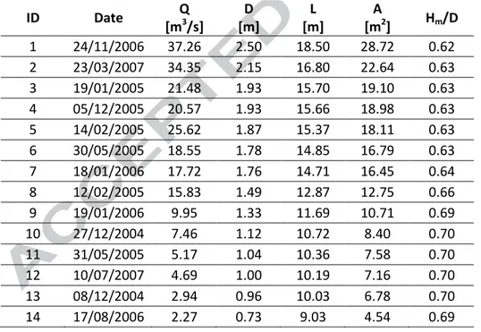
Table 2. Main hydraulic characteristics of the flood events observed at Mersch cross-section. 632 633 ID Date Q [m3/s] D [m] L [m] A [m2] Hm/D 1 24/11/2006 37.26 2.50 18.50 28.72 0.62 2 23/03/2007 34.35 2.15 16.80 22.64 0.63 3 19/01/2005 21.48 1.93 15.70 19.10 0.63 4 05/12/2005 20.57 1.93 15.66 18.98 0.63 5 14/02/2005 25.62 1.87 15.37 18.11 0.63 6 30/05/2005 18.55 1.78 14.85 16.79 0.63 7 18/01/2006 17.72 1.76 14.71 16.45 0.64 8 12/02/2005 15.83 1.49 12.87 12.75 0.66 9 19/01/2006 9.95 1.33 11.69 10.71 0.69 10 27/12/2004 7.46 1.12 10.72 8.40 0.70 11 31/05/2005 5.17 1.04 10.36 7.58 0.70 12 10/07/2007 4.69 1.00 10.19 7.16 0.70 13 08/12/2004 2.94 0.96 10.03 6.78 0.70 14 17/08/2006 2.27 0.73 9.03 4.54 0.69 634 635
28 Figures
636
Figure 1. Example of a generic half cross-section and associated reference system. 637
638
Figure 2. Parameters used to estimate the parameter W. 639
640
Figure 3. Areas of study: (a) Upper Tiber basin and (b) Alzette basin. 641
642
Figure 4. Topographical survey of the analyzed river sites. 643
644
Figure 5. Comparison between the observed bathymetry and the bathymetry reconstructed by means 645
of the proposed procedure (eq. 13) and by means of the procedure proposed by Moramarco et al. 646
(2013) (n: number of flood events for which observed, georeferenced flow width and water level 647
data were used for parameterization of eq.13). 648
649
Figure 6. Trend in the parameter W versus the number of events n used for its estimation. 650
651
Figure 7. Comparison between observed and estimated flow areas. 652
653
Figure 8. Comparison between the observed bathymetry and the bathymetry reconstructed by means 654
of the proposed procedure (eq. 13) (n: number of flood events for which observed, georeferenced 655
flow width and water level data were used for parameterization of eq.13). 656
657
Figure 9. Trend in the parameter W versus (depth of the water surface of generic flood event with 658
respect to the water surface associated with the largest/maximum observed flood event). 659
660
Figure 10. Comparison between observed and estimated discharges. 661
662 663
Figure1
Figure2
Figure3
Figure4
Figure5
Figure6
Figure7
Figure8
Figure9
Figure10
1 Highligths
A new method for estimating the cross-section bathymetric profile is proposed.
We apply the principle of maximum entropy to describe the depth distribution.
The parameterization of the procedure requires exclusively few geometric data.