Efficient Feasibility Analysis of Real-Time
Asynchronous Task Sets
Rodolfo Pellizzoni
Universit`a di Pisa and Scuola Superiore S. Anna, Pisa, Italy [email protected]
Abstract
Several schedulability tests for real-time periodic task sets scheduled under the Earliest Deadline First algorithm have been proposed in literature, in-cluding analyses for precedence and resource constraints. However, all avail-able tests consider synchronous task sets only, that are task sets in which all tasks are initially activated at the same time. In fact, every necessary and sufficient feasibility condition for asynchronous task sets, also known as task sets with offsets, is proven to be NP-complete in the number of tasks. We propose a new schedulability test for asynchronous task sets that, while being only sufficient, performs extremely better than available tests at the cost of a slight complexity increase. The test is further extended to task sets with resource constraints, and we discuss the importance of task off-sets on the problems of feasibility and release jitter. We then show how our methodology can be extended in order to account for precedence constraints and multiprocessor and distributed computation applying holistic response time analysis to a real-time transaction-based model. This analysis is finally applied to asymmetric multiprocessor systems where it is able to achieve a dramatic performance increase over existing schedulability tests.
Contents
Abstract iii
1 Introduction 1
2 System Model 5
2.1 Simple task model . . . 5
2.1.1 Resource usage . . . 8
2.2 Scheduling algorithms . . . 9
2.3 Transaction model . . . 11
3 Feasibility analysis for asynchronous task sets 13 3.1 Introduction . . . 13 3.1.1 Motivation . . . 14 3.2 System model . . . 15 3.3 Feasibility analysis . . . 15 3.4 Algorithm . . . 23 3.5 Experimental evaluation . . . 26 3.6 Conclusions . . . 28
4 Resource usage extension 31 4.1 Introduction . . . 31
4.2 Test extension . . . 32
4.3 Busy period length . . . 34
5 Offset Space Analysis 35 5.1 Introduction . . . 35
5.2 Task model and basic facts . . . 35
5.3 Phase-space construction and conversions . . . 37
5.4 Phase-space representation correctness . . . 40
5.5 Feasibility applications . . . 41
5.6 Conclusions . . . 45
6 Minimization of output jitter 47 6.1 Introduction . . . 47
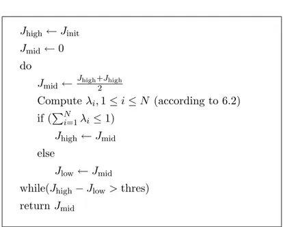
6.2 Polynomial time bounds . . . 49
6.3 Pseudo-polynomial time minimization . . . 50
6.4 Experimental evaluation . . . 51
6.5 Conclusions . . . 54
7 Response time analysis for EDF 55 7.1 Introduction . . . 55
7.2 Variation of the Palencia-Gonz`alez’s method . . . 56
7.3 New offset method . . . 60
8 Improved holistic analysis 63 8.1 Introduction . . . 63
8.2 Holistic Analyses . . . 64
8.3 Implementation Issues . . . 73
8.4 Experimental evaluation . . . 77
8.5 Deadline selection . . . 81
9 Heterogeneous multiprocessor systems 83 9.1 Introduction . . . 83
9.2 Multiple Coprocessors . . . 84
9.3 Preemptive Coprocessor . . . 85
9.4 Non Preemptive Coprocessor . . . 87
9.5 Resource usage . . . 91
9.5.1 Busy period length . . . 92
9.6 Deadline search algorithm . . . 93
9.7 Conclusions . . . 95
List of Figures
2.1 Transaction model. . . 11
3.1 Example of busy period. . . 16
3.2 Example synchronous task set . . . 17
3.3 Example task set, τ1(φ = 1, C = 2, D = 3, T = 4), τ2(φ = 0, C = 2, D = 3, T = 6) . . . 18
3.4 Example task set, τ1(φ = 0, T = 3), τ2(φ = 1, T = 4), τ3(φ = 2, T = 6) . . . 19
3.5 Sample code, 1 fixed task . . . 24
3.6 Sample code, 2 fixed tasks . . . 25
3.7 6 tasks, gcd = 10, deadline ∈ [0.3, 0.8]T . . . 27 3.8 6 tasks, gcd = 10, deadline ∈ [0.5, 1.0]T . . . 27 3.9 6 tasks, gcd = 5, deadline ∈ [0.3, 0.8]T . . . 29 3.10 10 tasks, gcd = 10, deadline ∈ [0.3, 0.8]T . . . 29 3.11 10 tasks, gcd = 10, deadline ∈ [0.5, 1.0]T . . . 30 3.12 20 tasks, gcd = 10, deadline ∈ [0.5, 1.0]T . . . 30 5.1 5 tasks, deadline ∈ [0.5, 1.0]T . . . 44 5.2 5 tasks, deadline ∈ [0.3, 0.8]T . . . 45
6.1 Sample code, polynomial time method . . . 50
6.2 10 tasks, 10 minimized jitters . . . 52
6.3 10 tasks, 5 minimized jitters . . . 52
6.4 10 tasks, 3 minimized jitters . . . 53
6.5 5 tasks, 5 minimized jitters . . . 53
8.1 Example of jitter extension. . . 66 vii
8.2 Holistic analysis example. . . 68
8.3 CDO iteration step. . . 71
8.4 Sample code, algorithm WCDO . . . 74
8.5 Sample code, algorithm MDO . . . 74
8.6 Sample code, algorithm NTO . . . 75
8.7 Sample code, algorithm TO . . . 76
8.8 5 transactions, 5 tasks per transaction, single processor . . . . 79
8.9 5 transactions, 5 tasks per transaction, two processors . . . . 79
8.10 5 transactions, 10 tasks per transaction, four processors . . . 80
8.11 5 transactions, 5 tasks per transaction, two processors . . . . 80
9.1 5 DSP tasks, dedicated coprocessors . . . 86
9.2 10 DSP tasks, dedicated coprocessors . . . 86
9.3 5 DSP tasks, shared preemptible coprocessor . . . 87
9.4 10 DSP tasks, shared preemptible coprocessor . . . 88
9.5 5 DSP tasks, shared non preemptible coprocessor . . . 90
List of Tables
3.1 Mean number of cycles, gcd = 10, deadline ∈ [0.3, 0.8]T . . . . 28 8.1 Mean number of steps, 5 transactions . . . 81
Chapter 1
Introduction
Real-time systems are computing systems that must react within precise time constraints to external events. Real-time systems are gaining more and more importance in our society since an increased number of control systems relies on computer control. Examples of such applications include production processes, automotive applications, telecommunication systems, robotics and military systems. The correct behaviour of a real-time system depends not only on computation results but also on the time at which the result is provided [32, 9]. Moving an actuator at the wrong time can be as disastrous as moving it in the wrong direction.
It is important to note that real-time computing does not correspond to fast computing. While the objective of fast computing is to minimize the average response time of each task, the objective of real-time computing is to meet the timing constraints of each task in the system. The most typical timing constraint for a task is a deadline, that is the maximum time at which the task must complete execution. In particular, a real-time system is said to be hard if missing a deadline may cause catastrophic consequences on the environment under control. Obviously, the average response time of the system has no effect on its correct behaviour in a real-time system.
A key world in real-time system theory is predictability [33]. In other words, we must be able to predict, based on hardware and software spec-ifications, the evolution of each task. Specifically, a hard real-time system must guarantee that all tasks remains feasible (meet their deadlines) even in the worst possible scenario. Unfortunately, most optimization techniques used for fast computing, especially on the hardware side, do not work well on real-time systems since they affect predictability. While deep proces-sor pipelining and caching enhance a task’s execution speed on average, in
the worst case they may actually introduce further delays. Furthermore, an increase of computational power or a decrease of execution time do not necessarily improve feasibility, at least in multiprocessor systems [17].
A real-time system typically consists of a set of concurrent tasks that compete over processor time. The system must thus implement a scheduling
algorithm that decides which task must be scheduled (executed) at each
time slot. In order to achieve predictable guarantees, schedulability tests must be developed for each scheduling algorithm. A schedulability test is an algorithm that given a task set returns a positive answer if the task set can be feasibly scheduled under its associated scheduling algorithm. This work introduces new schedulability tests for the well-know Earliest Deadline First (EDF) scheduling algorithm [24].
Chapter 2 introduces the system models that we will use in our work and presents a brief survey of available scheduling algorithms. We present both the standard periodic task model used in literature and the transaction model introduced in [25].
Chapter 3 presents our new schedulability test for asynchronous periodic task sets. Our main idea is the exploitation of task offsets; the offset of each task is the first time instant at which it is activated in the system. As we show by means of experimental evaluations, our technique clearly outper-forms the available tests in literature, although its computation complexity is also slightly higher.
Chapter 4 provides an extension of the test developed in Chapter 3 to the case of tasks sharing resources. In order to preserve predictability, a real-time system must implement a real-time resource access protocol that gives guarantees on the maximum time that a task may be blocked waiting for a resource. Our discussion is based on the widely used Stack Resource Protocol (SRP) [2].
Chapter 5 provides more insight into the relation between task offsets and feasibility. We presents a new offset representation and try to develop heuristics to choose task offsets in a quasi-optimal way. However, we debate that solving the latter problem is probably impossible, at least in polynomial time.
Chapter 6 presents a relevant problem in the field of real-time control systems, that of task output jitter. The test developed in Chapter 3 is then applied to the problem and compared to existing approaches.
In Chapters 7 and 8 we extend the offset methodology applied in Chapter 3 to the transaction model. This system model is particularly suitable to
3 represent systems in which a task may suspend itself for a certain time, and for distributed and multiprocessor systems. Since the schedulability test for this system model is quite complex, we split the discussion into two chapters. Chapter 7 covers the problem of response time analysis for transaction systems scheduled under EDF, while Chapter 8 is about the holistic analysis of transaction sets with dynamic offsets. In both chapters we present our original contribution to the problem and in Chapter 8 we even show experimental results.
In Chapter 9 the transaction-based test is applied to the case of
heteroge-neous multiprocessor systems, or asymmetric multiprocessors. Experimental
evaluations show how our test, combined to suitable heuristics, is able to dramatically outperforms all other analysis known so far.
Finally, in Chapter 10 we offer some conclusive thoughts about our major results and possible future work.
Chapter 2
System Model
We will start our discussion by introducing system models and general def-initions that will be needed in the rest of our work. We will basically use two different models: a simple task model, which is very similar to the stan-dard literature real-time task set model, and a transaction model, which was first introduced in [25] and is suitable to represent a variety of situations in which dependencies between tasks arises. These two models will be covered in Section 2.1 and 2.3, while in Section 2.2 we will provide a quick overview of the main results about feasibility for both fixed and dynamic priority scheduling.
2.1
Simple task model
We will now introduce our basic task model. We assume that a task set T made of N different tasks {τ1, . . . , τN} must be scheduled in a hard real-time
system. Barring exceptions, we will suppose that all tasks are executed on a single processor.
Each task τi consists of an infinite series of jobs {τi1, . . . , τij, . . .}. Each
job τij consists of a thread of execution that must run for at most Ci time units; such value is called the worst-case computation time of task τi, and we suppose that it does not change between jobs of the same task. A task is said to be periodic if each successive job τij is activated (i.e., presented to the system) at a fixed time interval Ti, which is called the task’s period. A task is said to be aperiodic if it is not periodic. Note that we can’t provide any guarantee about aperiodic tasks since no bound on the interval between successive activations of an aperiodic task is provided; any number
of jobs may be activated inside a time interval of any length. Therefore, in order to introduce aperiodic tasks in a hard-real time system we must execute them inside a special periodic task that is typically called a server. We will not be concerned with servers in the remainder of this work. A special case of aperiodic tasks worth mentioning is that of sporadic tasks. Successive jobs of a sporadic task are activated at intervals that are at least equal to a given minimum inter-arrival time Ti. In this case the lower bound on the interval permits to develop real-time guarantees on the system, therefore we are not forced to execute sporadic tasks inside a server; note, however, that in general a sporadic task performs worse than a periodic task of period equal to the minimum inter-arrival time of the sporadic task, meaning that analyses developed for periodic tasks (such as those introduced in the following chapters) cannot be always extended to sporadic tasks. In what follows we will be mainly interested in the study of periodic task sets.
A task is characterized by a tuple (φi, Ci, Ti, Di, Ji), where:
• φi is the task’s offset. The offset is the first time at which a job of the task is activated.
• Ci is the worst-case execution time of the task; note, however, that in most practical applications computing Ci is far from being easy.
• Tiis either the task’s period (for periodic tasks) or the task’s minimum inter-arrival time (for sporadic tasks).
• Di is the task’s relative deadline. A job is feasible only if it finishes at most Di time units after its activation.
• Ji is the task’s release jitter.
Each job τij is thus activated at time aij = φi + jTi and must finish before or at its absolute deadline dij = aij+ Di. If we let fij be the time at which job τij finishes execution (called the finishing time or the completion
time of the job), the feasibility condition for the task set becomes: ∀1 ≤ i ≤ N, ∀j ≥ 1, fij ≤ dij. Each task τi can further experience a release jitter Ji. If the release jitter is not zero, then the release time of job τij (i.e., the time at which the task is ready to be scheduled) is different from its activation time, being comprised between aij and aij + Ji. If not told otherwise, we will suppose that all release jitters are equal to zero, and thus the release time of a job corresponds to its activation time; in this case we will use the two terms interchangeably.
2.1. SIMPLE TASK MODEL 7 A task set is said to be incomplete if the task offsets are not specified. This basically means that we are required to make a pessimistic assumption on offsets. A task set is said to be complete if task offsets are given; it is also called a task set with offsets. In this case, the task set is said to be
synchronous if all offsets are equal to zero. A task said is asynchronous if
it is not synchronous. Note that given an asynchronous task set T we can always define the corresponding synchronous task set as T0 = {τ0
1, . . . , τN0 }, where for every task τi0 : φ0i= 0, Ci0 = Ci, Ti0= Ti, Di0 = Di, Ji0= Ji.
We will suppose that all task parameters are expressed by integer num-bers. It can be proven that in this case, if a feasible schedule exists, then a feasible integer schedule (i.e. a schedule in which all preemption times are expressed by integer numbers) exists too [4]; this property is known as the integral boundary constraint. We can thus restrict ourselves to consider only integer schedules. A schedule will thus be a function σ : N → T ∪ {∅} that assigns to each time slot t a task τi, or the symbol ∅ to indicate that the processor is idle. Note that considering all task parameters and thus all activation and preemption times to be integer is not a major limitation for at least two reasons. The first one is that, if some parameters were originally expressed by rational numbers, we can always reduce them to integers mul-tiplying them by their common denominator; there seems to be no reason to choose irrational values. The second one is that all time values inside the system, due to practical implementation, must be multiples of a basic clock tick.
We further define:
1. Ui = CTii is the utilization of task τi; the utilization is a measure of how much computation time the task requires.
2. U =PNi=1Ui is the total utilization of task set T . 3. Φ = max{φ1, . . . , φN} is the largest offset.
4. function gcd(Ti, Tj) is the greatest common divisor between two peri-ods Ti and Tj; gcd(Ti, . . . , Tj) is the same among periods T1, . . . , Tj. 5. function lcm(T1, Tj) is the least common multiple between two periods
T1, Tj, and lcm(Ti, . . . , Tj) is the same among periods T1, . . . , Tj. 6. H = lcm{T1, . . . , TN} is the hyperperiod of T . 7. ηi(t1, t2) = ³j t2−φi−Di Ti k − l t1−φi Ti m + 1 ´
τi with release time greater than or equal to t1 and deadline less then or equal to t2 [5].
Also, notation (x)0 will be used as an abbreviation of max(x, 0).
An essential concept is that of busy period. A busy period [t1, t2) is an interval of time in which the processor is always busy, that is: ∀t ∈ [t1, t2), σ(t) 6= ∅.
In all the figures showing a schedule, we represent the execution of each task on a separate horizontal line. Upward arrows represent release times while downward arrows represent absolute deadlines.
2.1.1 Resource usage
In our simple task model, tasks can be synchronized using shared resources. This synchronization model is commonly used in shared memory systems, as many real-time systems and most embedded systems are. We consider a set R of R shared resources ρ1, . . . , ρR. To simplify our presentation, only single-unit resources are considered, although there are ways to consider the case of multi-unit resources [2].
Any task τi is allowed to access shared resources only through mutually exclusive critical sections. Each critical section ξij is described by a 3-ple (ρij, φij, Cij), where:
1. ρij is the resource being accessed;
2. φij is the earliest time, relative to the release time of job τij, that the task can enter ξij;
3. Cij is the worst-case computation time of the critical section.
Critical sections can be properly nested in any arbitrary way, as long as their earliest entry time and worst-case computation time is known. Note that our model, which was first proposed in [23], is actually slightly different from the classic one in literature in that it requires earliest entry time to be known. We feel, however, that such a request should not pose too great a problem in practical applications.
Since critical sections must be executed in a mutually exclusive way to guarantee synchronization, a task can’t enter a critical section using a resource ρk if another task is using the same resource. This means that a task can be forced to wait until another one finishes executing a critical section before restarting execution. Such a task is said to be blocked by the task holding the resource.
2.2. SCHEDULING ALGORITHMS 9
2.2
Scheduling algorithms
Two classes of scheduling algorithms have been proposed in literature: fixed
priority scheduling (FPS) and dynamic priority scheduling (DPS). Note that
all the following results are valid if no resource synchronization is considered. In fixed priority scheduling, each task τiis assigned a fixed priority value. At each time instant, the scheduler schedules the active task with the highest priority (a task is said to be active if its current job has been released but has not finished yet and it is not blocked). Under the Rate Monotonic algorithm (or briefly RM), each task is assigned a priority that is inversely proportional to its period. Rate Monotonic is proven to be optimal (meaning that if a task set is schedulable under any algorithm, it is schedulable under RM) among all fixed priority algorithms in the case where task deadlines are equal to task periods [24]. In the case in which deadlines are less than or equal to the periods, the Deadline Monotonic algorithm (or DM), where each task is assigned a priority inversely proportional to its relative deadline, is optimal instead [22].
In dynamic priority scheduling, each task is also assigned a priority value, but such value can be dynamically adjusted. For example, under the Earliest Deadline First algorithm (or briefly EDF), each task is assigned a priority inversely proportional to the absolute deadline of its current job; priorities are thus changed each time a new job is activated. EDF is proven to be optimal among all scheduling algorithms [13].
If deadlines are equal to the periods, than the condition U ≤ 1 is a necessary a sufficient feasibility condition under EDF. Such a condition is only sufficient if deadlines are less than the periods. Under RM, two similar feasibility bounds on utilization can be provided [24, 8]:
U ≤ N (2N1 − 1)
and Y
1≤i≤N
(Ui+ 1) ≤ 2 but these conditions are only sufficient.
Necessary and sufficient feasibility conditions exists for both DM and EDF when deadlines are less than or equal to the periods and the task set is synchronous [4, 1]. The EDF schedulability test, known as
proces-sor demand criterion, will be analyzed in Chapter 3. While these tests are
more extensive in terms of computation time. The computation complexity of a schedulability test is usually computed as a function of the number of tasks. The sufficient and necessary tests for both DM and EDF have
pseudo-polynomial complexity, meaning that they have complexity pseudo-polynomial in
the number of tasks but also proportional to some task parameters. Intu-itively, a pseudo-polynomial complexity is somehow worse than a polynomial one but better than an exponential one.
Scheduling is much more complex when tasks are allowed to share re-sources. In fact, if plain EDF or RM/DM are applied, a higher priority task can be blocked indefinitely by lower priority tasks. In order to provide real-time guarantees, the scheduling algorithm must be modified to include a resource access protocol. The protocol usually gives an upper bound Bi, called the maximum blocking time, to the time a task τi can be blocked waiting for lower priority tasks. Many different resource synchronization protocols have been proposed for both EDF and RM/DM [2, 12, 19, 29].
Given a maximum blocking time Bi for each task τi, the previous schedu-lability tests can be updated to include the effect of blocking times. The feasibility condition based on utilization for EDF becomes:
∀1 ≤ i ≤ N, X
1≤j≤i
Uj+BTi i
≤ 1
where tasks are assumed to be ordered by increasing relative deadline. The same holds for RM, except that the bound is not 1 but i(21i−1). In Chapter
4 we will see how the processor demand criterion can be applied to the case of resource usage.
In general, DPS offers better results over FPS in term of feasibility. The main drawback of dynamic priority scheduling is in its increased conceptual complexity over fixed priority scheduling. This is the main reasons why most if not all commercially available real-time systems today implement only FPS. Secondary DPS problems include a slightly increased scheduling overhead and worse predictability in case of overloading (an overload occurs if for some reason a task executes longer than its worst-case computation time). However, dynamic priority scheduling is progressively gaining im-portance and most new research operating systems typically offer a choice between RM/DM and EDF scheduling.
In the remainder of this work, EDF is assumed as the scheduling algo-rithm.
2.3. TRANSACTION MODEL 11 ai3 ai2 ai1 ai Ti Ci3 Ci2 Ci1 Ji3 Ji2 Ji1 Ti di3 φi3 di2 φi2 di1 φi1
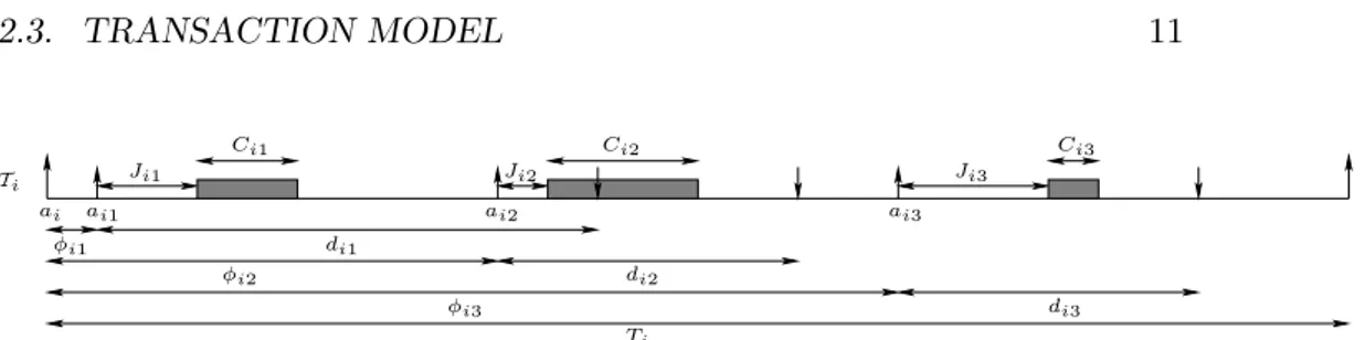
Figure 2.1: Transaction model.
2.3
Transaction model
In this section we introduce a general transaction model that will be used in Chapter 7 and in Chapters 8 and 9 with small changes.
We will consider a real-time system made of M sets of periodic tasks that we will name transactions. Each transaction Ti is characterized by period
Ti and offset φi such that the kth instance of each transaction is activated at time ak
i = φi + kTi. Furthermore, each transaction Ti is composed of
Ni tasks τi1, . . . , τiNi. Each task τij is characterized by an offset φij, a
computation time Cij, a relative deadline dij and a release jitter Jij. The
kth instance (that is, the kth job) of task τ
ij, that we will denote τijk, has an activation time ak
ij = aki + φij, but its release time can be delayed up to a maximum release jitter Jij. The job takes up to Cij units of computation times to be completed and must be finished before its absolute deadline
ak
ij + dij. We will further define Dij to be the global relative deadline of task τij, that is the deadline relative to the activation time of transaction
Ti: Dij = dij + φij. We will assume that tasks are statically assigned to be scheduled on P different processors: in particular, tasks pertaining to the same transaction may be executed on different processors. Figure 2.1 shows the model for a transaction Ti.
The worst-case relative response time rij of a task is the greatest differ-ence between the finishing time of a job τk
ij and its activation time akij. The worst-case global response time Rij is the greatest difference between the finishing time of a job of τij and the activation time of its transaction, thus
Rij = rij+ φij. Note that a real-time transaction system is feasible if and only if for all tasks of all transactions, the worst-case relative response time is less than or equal to the relative deadline.
Tasks are allowed to share resources in mutually exclusive way using critical section as addressed in Section 2.1.1. Each critical section ξijk is described by a 3-ple (ρijk, φijk, Cijk), where:
1. ρijk is the resource being accessed;
2. φijk is the earliest time, relative to the activation time of τijk, that the task can enter ξijk;
3. Cijk is the worst-case computation time of the critical section.
The effect of resource usage is that a task running on one processor can be blocked by both lower priority tasks running on the same processor and by tasks running on a different processor; the maximum blocking time for task
Chapter 3
Feasibility analysis for
asynchronous task sets
3.1
Introduction
As we said in the previous Chapter 2, in single processor systems the Earliest Deadline First scheduling algorithm is optimal [13], in the sense that if a task set is feasible, then it is schedulable by EDF. Therefore, the feasibility problem on single processor systems can be reduced to the problem of testing the schedulability with EDF.
The feasibility problem for a set of independent periodic tasks to be scheduled on a single processor has been proven to be co-NP-complete in the strong sense [21, 5]. Leung and Merril [21] proved that it is necessary to analyze all deadlines from 0 to Φ + 2H. Baruah et al. [5] proved that, when the system utilization U is strictly less than 1, the Leung and Merril’s condition is also sufficient.
Under certain assumption, the problem becomes more tractable. For example, if deadlines are equal to period, a simple polynomial test has been proposed by Liu and Layland in their seminal work [24]. If the deadlines are less than or equal to the periods and the task set is synchronous (i.e. all tasks have initial offset equal to 0), then a pseudo-polynomial test has been proposed by Baruah et al. [4, 5].
In the case of asynchronous periodic task sets, any necessary and suf-ficient feasibility test requires an exponential time to run. However, it is possible to obtain a sufficient test by ignoring the offsets and considering the task set as synchronous. Baruah et al. [5] showed that, given an
chronous periodic task set T , if the corresponding synchronous task set T0 (obtained by considering all offsets equal to 0) is feasible, then T is feasible too. However, if T0 is not feasible, no definitive answer can be given on
T . In some case this sufficient test is quite pessimistic, as we will show in
Section 3.5.
The basic idea behind Baruah’s result is based on the concept of busy
period. A busy period is an interval of time where the processor is never idle.
If all tasks start synchronously at the same time t, the first deadline miss (if any) must happen in the longest busy period starting from t. Unfortunately, when tasks have offsets, it may not be possible for them to start at the same time. Hence, in case of asynchronous task sets, we do not know where the deadline miss might happen in the schedule.
In this chapter, a new sufficient pseudo-polynomial feasibility test for asynchronous task set is proposed. Our idea is based on the observation that the patterns of arrivals of the tasks depend both on the offsets and on the periods of the tasks. By computing the minimum possible distance between the arrival times of any two tasks, we are able to select a small group of critical arrival patterns that generate the worst-case busy period. Our arrival patterns are pessimistic, in the sense that some of these patterns may not be possible in the schedule. Therefore, our test is only sufficient. However, experiments show that our test greatly reduces pessimism with respect to previous sufficient tests.
3.1.1 Motivation
The problem of feasibility analysis of asynchronous task sets can be found in many practical applications. For example, in distributed systems a
trans-action consists of a chain of tasks that must execute one after the other
and each task can be allocated to a different processor. A transaction is usually modelled as a set of tasks with offsets, such that the first task in the chain has offset 0, the second task has an offset equal to the minimal response time of the first task, and so on. Furthermore, each task is assigned a non-zero release jitter. In this way, the problem of feasibility analysis of the entire system is divided into the problem of testing the feasibility on each node. The holistic analysis [34, 31] iteratively computes the worst-case response time of each task and updates the start time jitter of the next task in the chain, until the method converges to a result. The methodology has been recently extended by Palencia and Gonz´alez Harbour [26], and will be further explored in Chapter 7 and 8.
3.2. SYSTEM MODEL 15 Another important field of application is concerned with the problem of minimizing the output jitter of a set of periodic tasks. The output jitter is defined as the distance between the response time of two consecutive in-stances of a periodic task. Minimizing the output jitter is a very important issue in control systems. Baruah et al. [3] presented a method for reducing the output jitter consisting in reducing as much as it is possible the rela-tive deadlines of the tasks without violating the feasibility of the task set. However, tasks are considered synchronous. In Chapter 6 we will extend the method to asynchronous task sets.
3.2
System model
The simple task model introduced in Section 2.1 is used in this chapter. Task set are supposed to be complete with no release jitter and deadlines less than or equal to the periods; no resource constraint is considered. The analysis proposed in this chapter will be extended to the case of resource usage in the following Chapter 4.
3.3
Feasibility analysis
In this section, we will first show the fundamental results for the problem of feasibility analysis of periodic task sets on single processor systems. Then we present our idea and prove it correct.
Our analysis is based on the processor demand criterion [5, 9]. The
processor demand function is defined as df (t1, t2) =
N X i=1
ηi(t1, t2)Ci.
It is the amount of time demanded by the tasks in interval [t1, t2) that the processor must execute to ensure that no task misses its deadline. Intuitively, the following is a necessary condition for feasibility:
∀ 0 ≤ t1 < t2 : df (t1, t2) ≤ t2− t1.
In plain words, the amount of time demanded by the task set in any interval must never be larger than the length of the interval.
Now, we report two fundamental results on the schedulability analysis of a periodic task set with EDF. The proofs of these results are not the original
τ1
τ2
τ3
t1 t2
Figure 3.1: Example of busy period.
ones. They have been rewritten for didactic purposes. In fact, by following the proofs, the reader will understand the basic mechanism underlying our methodology.
We will now start by reproducing the following important lemma. Lemma 1 ([5]) Task set T is feasible on a single processor if and only if:
1. U ≤ 1, and
2. ∀ 0 ≤ t1 < t2≤ Φ + 2H : df (t1, t2) ≤ t2− t1. Proof.
Both conditions are clearly necessary. By contradiction. Suppose both conditions hold but T is not feasible. Consider the schedule generated by EDF. It can be proven [5, 21] that since U ≤ 1 and the task set is not feasible, some deadline in (0, Φ + 2H] is missed. Let t2 be the first instant at which a deadline is missed, and let t1 be the last instant prior to t2 such that either no jobs or a job with deadline greater than t2 is scheduled at
t1 − 1. By choice of t1, it follows that [t1, t2) is a busy period and all jobs that are scheduled in [t1, t2) have arrival times and deadlines in [t1, t2] (see Figure 3.1). It also follows that at least one job with deadline no later than
t2 must be released exactly at t1, otherwise either a job with deadline greater than t2 or no job would be scheduled at t1. Since there is no idle time in [t1, t2) and the deadline at t2 is missed, the amount of work to be done in [t1, t2) exceeds the length of the interval. By definition of df , it follows that
df (t1, t2) > t2− t1, which contradicts condition 2. 2
By looking at the proof, it follows that it is sufficient to check the values of df (t1, t2) for all times t1 that corresponds to the release time of some job. In the same way, we can check only those t2 that correspond to the absolute deadline of some job.
We will now prove that for a synchronous task set the first deadline miss, if any, is found in the longest busy period starting from t1 = 0. Thus, it
3.3. FEASIBILITY ANALYSIS 17 τ1 τ2 τ3 τ1 τ2 τ3 t1+0 5 10 15 20 25 t02 t2 30 31
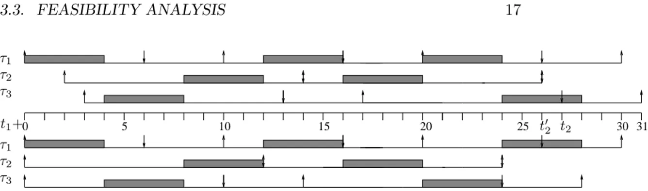
Figure 3.2: Example synchronous task set
suffices to check all deadlines from 0 to the first idle time. The idea is that, given any busy period starting at t1, we can always produce a “worst-case” busy period “pulling back” the release times of all tasks that are not released at t1, so that all tasks are released at the same time. Figure 3.2 shows the idea for a task set of N = 3 tasks with τ1(C = 4, D = 6, T = 10), τ2(C = 4, D = 12, T = 12), τ3(C = 4, D = 10, T = 14) where task τ1 is released at
t1. In the lower part of the figure, we show the situation where tasks τ2 and
τ3 are “pulled back” until their first release time coincides with t1.
Theorem 1 ([5]) A synchronous task set T is feasible on a single processor
if and only if:
∀L ≤ L?, df (0, L) ≤ L
where L is an absolute deadline and L? is the first idle time in the schedule. Proof. The condition is clearly necessary. By contradiction. Consider the schedule generated by EDF. Suppose that a deadline is missed, and let [t1, t2) be a busy period as in the previous lemma. We already proved that there is at least one task that is released exactly at t1. Let τi be one such task, so that t1 = aim for some m, and τk be the task whose deadline dkp is not met (note that it could be i = k). By following the same reasoning as in Lemma 1, we obtain df (t1, t2) > t2− t1.
Now consider a task τj, j 6= i, k, and suppose that the first release time of a job of τj is ajl> t1. The new schedule generated by “pulling back” all releases of task τj of ajl− t1 is still unfeasible. In fact, since all absolute deadlines of task τj are now located earlier, the number of jobs of τj in [t1, t2] could be increased: ηj0(t1, t2) ≥ ηj(t1, t2). Thus
PN
i=1,i6=jηi(t1, t2)Ci+
η0
j(t1, t2)Cj ≥
PN
i=1ηi(t1, t2)Ci > t2− t1 (see task τ2 in Figure 3.2). Now consider task τk, and suppose that k 6= i. Let akl be the first release time
τ1
τ2
0 1 2 3 4 5 6 7 8 9 10 11 12 13
Figure 3.3: Example task set, τ1(φ = 1, C = 2, D = 3, T = 4), τ2(φ = 0, C = 2, D = 3, T = 6)
of τk after t1. By moving all releases back of akl− t1, we also move back its deadlines. Let d0
kp ≤ dkp be the new deadline. We shall consider two possible cases. First, suppose that for each deadline djq ≤ dkp, j 6= k, it
still holds djq ≤ d0kp. Then df (t1, t02 = d0kp) = df (t1, t2) > t2− t1 > t02− t1 and the new task set is not feasible. Second, suppose that djq is the largest deadline in [t1, t2] such that d0kp< djq ≤ dkp. Consider the new busy period [t1, t02 = djq). Then df (t1, t20) = df (t1, t2), but we obtain t02 ≤ t2 and thus the new task set is not feasible (see Figure 3.2, where k = 3 and j = 1).
Therefore, by moving back all tasks such that their first release time is at t1 we obtain an unfeasible schedule where all tasks are released at t1. Thus if a deadline is not met inside any busy period, then a deadline must not be met inside the busy period starting at 0. Since this contradicts the hypothesis, the theorem holds. 2
Baruah et al. [5] showed that for U < 1 the analysis has complexity
O
³
N1−UU maxNi=1{Ti− Di} ´
.
The previous theorem does not hold in the case of an asynchronous task set. It still gives a sufficient condition, in the sense that if the hypothesis holds for the corresponding synchronous task set, than the original asyn-chronous task set is feasible. However the condition is no longer necessary. Consider the feasible task set in Figure 3.3. It is easy to see that no instant
t1 exists such that both tasks are released simultaneously. We can still use a pessimistic analysis by considering the corresponding synchronous task set, but in the case of Figure 3.3 this wouldn’t work since it can be easily seen that the corresponding synchronous task set is not feasible. Checking all busy periods in [0, Φ + 2H] is possible but would imply an exponential complexity.
Our main idea is as follow. Since there is always an initial task that is released at t1, we build a new task set Ti0 for each possible initial task
τi, 1 ≤ i ≤ N . Since τi is released at the beginning of the busy period, we fix φ0
3.3. FEASIBILITY ANALYSIS 19 τ1 τ2 τ3 a11 a12 a13 a14 a15 a21 a22 a23 a24 a31 a32 a33 0 1 2 3 4 5 6 7 8 9 10 11 12 13 14
Figure 3.4: Example task set, τ1(φ = 0, T = 3), τ2(φ = 1, T = 4), τ3(φ = 2, T = 6)
can then “pull back” each other task τj by setting φ0j to the minimum time distance between any activation of τi and the successive activation of τj in the original task set T . We will use the following Lemma:
Lemma 2 Given two tasks τi and τj, the minimum time distance between
any release time of task τi and the successive release time of task τj is equal
to: ∆ij = φj− φi+ l φi− φj gcd(Tj, Ti) m gcd(Tj, Ti)
Proof. Note that for each possible job τim and τjl, ajl− aim = φj− φi+
lTj− mTi. Thus ∀l ≥ 0, ∀m ≥ 0, ∃K ∈ Z, ajl− aim= φj− φi+ K gcd(Tj, Ti). By imposing ajl≥ aim, we obtain K ≥ l φi−φj gcd(Tj,Ti) m . By simple substitution, we obtain the lemma. 2
Definition 1 Given task set T , T0
i is the task set with the same tasks as T
but with offsets:
φ0i = 0
φ0j = ∆ij ∀j 6= i, 1 ≤ j ≤ N
Consider the example of Figure 3.4. By setting i = 1 we obtain φ0 1 = 0, φ02 = a23− a14= 0 and φ03 = a31− a11= 2.
We will now prove that, to assess the feasibility of T , it suffices to check that, for every task set T0
i, all deadlines are met inside the busy period starting from time 0.
Theorem 2 Given task set T with U ≤ 1, scheduled on a single processor,
if ∀ 1 ≤ i ≤ N all deadlines in task set T0
i are met until the first idle time,
Proof. By contradiction. Consider the schedule generated by EDF. Sup-pose that a deadline is not met for task set T , and let [t1, t2) be the busy period as defined in Lemma 1. We already proved that there is at least one task that is released at t1, let it be τi. From Lemma 2, it follows that for every τj, j 6= i, the successive release time is ajl ≥ t1+ ∆ij. By following the same reasoning as in Theorem 1, we can “pull back” every task so that its first release time coincides with its minimum distance from t1, and the resulting schedule is still unfeasible. Let σi(t) be the new resulting schedule. Now, observe that, from t1 on, the new schedule σi(t) is coincident with the schedule σ0
i(t) generated by task set Ti0 from time 0: ∀t ≥ t1 : σi(t) =
σ0i(t − t1). Therefore, there is a deadline miss in the first busy period in the schedule generated by T0
i, against the hypothesis. Hence, the theorem follows. 2
Note that Theorem 2 gives us a less pessimistic feasibility condition that Theorem 1. As an example, consider the task set in Figure 3.3. According to Theorem 2 the task set is feasible, while Theorem 1 gives no result.
However Theorem 2 gives only a sufficient condition. For example, con-sider the following task set: τ1(φ = 0, C = 1, D = 2, T = 5), τ2(φ = 1, C = 1, D = 2, T = 4), τ3(φ = 2, C = 1, D = 2, T = 6). By analyzing the schedule, it can be seen that it is feasible, but Theorem 2 fails to give any result. The reason can be easily explained. When we “pull back” the tasks to their min-imum distance from τi, we are not considering the cross relations between them. In other words, it may not be possible that the pattern of release times analyzed with Theorem 2 are found in the original schedule of T . We are considering only N patterns, but they are pessimistic.
In order to reduce the pessimism in the analysis, we can generalize The-orem 2 in the following way. Instead of fixing just the initial task τi, we can also fix the position of other tasks with respect to τi and then minimize the offsets of all the remaining tasks with respect to the fixed ones. The following lemma provides more insight into the matter.
Lemma 3 The time distance between any release time ail of task τi and the
successive release time ajp of task τj assumes values inside the following set: ½ ∆ij(k) | ∀ 0 ≤ k < gcd(TTj i, Tj) ¾ where ∆ij(k) = » φi+ kTi− φj Tj ¼ Tj− (φi+ kTi− φj)
3.3. FEASIBILITY ANALYSIS 21 Proof. Consider release time ail and let ajp be the first successive release time of task τj. Since ajpis greater than or equal to ail, it must be φj+pTj ≥
φi+lTi. But since ajpis the first such release, we obtain p = l φi+lTi−φj Tj m and ajp−ail= » φi+lTi−φj Ti ¼
Tj−(φi+lTi−φj). To end the proof it suffices to note that the value of ajp− ail as a function of l is periodic of period Tj
gcd(Ti,Tj). In fact: » φi+(l+Kgcd(Ti,Tj )Ti )Ti−φj Tj ¼ Tj − ³ φi + ³ l + K Tj gcd(Ti,Tj) ´ Ti ´ + φj = » φi+lT+Kgcd(Ti,Tj )Tj Ti −φj Tj ¼ Tj− ³ φi+ lTi+ K TjTi gcd(Ti,Tj) ´ + φj = ajp− ail. 2 Therefore, after fixing the first task τi we can fix another task τj to one of the values of Lemma 3. Now, if we want to fix a third task, we must be careful to select a time instant that is compatible with the release times of both τi and τj. The basic idea, explained in the following lemma, is to consider τi and τj as a single task of period lcm(Ti, Tj) and offset φi+ kTi. To generalize the notation, we denote with i1 the index of the first task that is fixed, with i2 the index of the second task, and so on, until iM that denotes the index of the last task to be fixed.
In what follows, notation lcmijdenotes the least common multiple among periods Ti, . . . , Tj, and gcdij will be used in the same way for the greatest common divisor.
Lemma 4 Let ai1l1 be any release time of task τi1, and let ∆i1i2(k1) be the
distance between ai1l1 and the successive release time of task τi2. The time
distance between ai1l1 and the successive release time of task τi3 assumes
values inside the following set:
½ ∆i1i2i3(k2) | ∀ 0 ≤ k2 < Ti3 lcm(Ti3, gcd(Ti1, Ti2)) ¾ where ∆i1i2i3(k2) = » φi1 + k1Ti1 + k2lcm(Ti1, Ti2) − φi3 Ti3 ¼ Ti3−(φi1+k1Ti1+k2lcm(Ti1, Ti2)−φi3)
Proof. Since the time difference between ai1l1 and the successive release
time ai2l2 of τi2 must be equal to ∆i1i2(k1), not all values of l1are acceptable.
Indeed, it must hold l1 ≡ k1mod ³
Ti2 gcd(Ti1,Ti2)
´ .
Let τi1i2 be a task with period Ti1i2 = Ti1
Ti2
gcd(Ti1,Ti2) = lcm(Ti1, Ti2) and
offset φi1i2 = φi1 + k1Ti1. All acceptable release times ai1l1 correspond to
the release times of task τi1i2. We can then apply Lemma 3 to τi1i2 and τi3
obtaining ∆i1i2i3. 2
Lemma 5 The time distance between any release time ai1l1 of task τi1 and the successive release time of task τip, given ai2l2−ai1l1 = ∆i1i2(k1), . . . , aip−1lp−1−
ai1l1 = ∆i1...ip−1(kp−2), assumes values inside the following set:
½ ∆i1...ip(kp−1) | ∀ 0 ≤ kp−1< Tip lcm(Tip, gcdi1ip−1) ¾ where ∆i1...ip(kp−1) = » φi1+ Pp−1 q=1kqlcmi1iq− φip Tip ¼ Tip− (φi1+ p−1 X q=1 kqlcmi1iq− φip)
Proof. The proof can be obtained by induction, reasoning in the same way as in Lemma 4. 2
Lemma 6 The minimum time distance between any release time ai1l1 of task τi1 and the successive release time of task τj, given ai2l2 − ai1l1 =
∆i1i2(k1), . . . , aiMlM − ai1l1 = ∆i1...iM(kM −1), is equal to:
∆i1...iMj = φj−φi1− M −1X q=1 kqlcmi1iq+ »φ i1 + PM −1 q=1 kqlcmi1iq − φj gcd(Tj, lcmi1iM) ¼ gcd(Tj, lcmi1iM)
Proof. Reasoning in the same way as in Lemma 4 and 5, all acceptable release times ai1l1 must correspond to the release times of a task τi1...iM with
period Ti1...iM = lcmi1iM and offset φi1...iM = φi1+
PM −1
q=1 kqlcmi1iq. We can
then apply Lemma 2 to τi1...iM and τj obtaining ∆i1...iMj. 2
Following the same line of reasoning as in Theorem 2, we now define task set T0
i1...iMk1...kM −1 in the same way as T
0
i before. Definition 2 Given task set T , T0
i1...iMk1...kM −1 is the task set with the same
tasks as T but with offsets: φ0i1 = 0
3.4. ALGORITHM 23 .. . ... ... φ0ip = ∆i1...ip(kp−1) .. . ... ... φ0iM = ∆i1...iM(kM −1) φ0j = ∆i1...iMj ∀j 6= i1, . . . , iM, 1 ≤ t ≤ N
Finally, we generalize Theorem 2 to the case of M fixed tasks.
Theorem 3 Given task set T with U ≤ 1, to be scheduled on a single
pro-cessor, let M be a number of tasks, 1 ≤ M < N . If ∀τi1, 1 ≤ i1 ≤ N, ∀τi2 6= τi1, 1 ≤ i2 ≤ N, . . . , ∀τiM 6= τi1, τi2, . . . , τiM −1, 1 ≤ iM ≤ N, ∀k1, 0 ≤ k1 < Ti2 gcd(Ti1, Ti2), ∀k2, 0 ≤ k2 < gcd(T Ti3 i3, lcm(Ti1, Ti2)) , . . . , ∀kM −1,0 ≤ kM −1 < TiM gcd(TiM, lcmi1iM −1)
, all deadlines in task set T0
i1...iMk1...kM −1 are met until
the first idle time, then T is feasible.
Proof. By contradiction. Consider the schedule generated by EDF. Sup-pose that a deadline is missed and let [t1, t2) be the busy period as in the proof of Lemma 1. We choose i1 such that t1 = ai1l1 for some l1. Next, we
choose any distinct indexes i2, . . . , iM and any values k1, . . . , kM −1as in Lem-mas 3, 4, 5, and compute the corresponding distances ∆i1i2(k1), . . . , ∆i1...iM(kM −1)
from t1. These tasks are fixed and will not be “pulled back”. For the re-maining tasks, we “pull back” their release times as much as it is possible: for every non-fixed task τj we set the distance from t1 equal to ∆i1...iMj. By
following the same reasoning as in Theorem 2, it can be easily proven that a deadline is still missed in the new generated schedule σ(t). Note that, from
t1 on, the schedule σ(t) is coincident with the schedule σ0(t) generated by task set T0
i1...iMk1...kM −1 from time 0: ∀t ≥ t1 : σ(t) = σ
0(t − t
1). Hence, a deadline is missed in the first busy period of σ0(t), against the hypothesis.
2
3.4
Algorithm
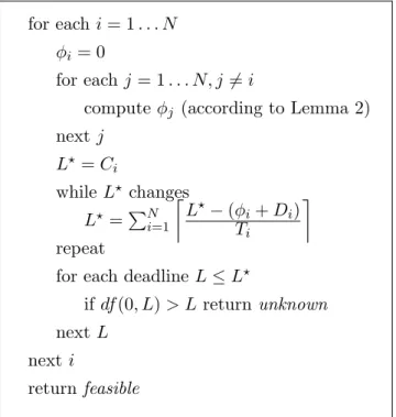
Theorem 2 gives us a new feasibility test for asynchronous task sets with
U < 1 on single processor systems. For each initial task τi we first compute the minimal offset φj for each j 6= i and the length L? of the busy period.
for each i = 1 . . . N
φi= 0
for each j = 1 . . . N, j 6= i
compute φj (according to Lemma 2) next j L? = C i while L? changes L?=PN i=1 » L?− (φi+ Di) Ti ¼ repeat
for each deadline L ≤ L?
if df (0, L) > L return unknown next L
next i
return feasible
Figure 3.5: Sample code, 1 fixed task
Then we check that each deadline L less than or equal to L? is met. The pseudo code is given in Figure 3.5.
Note that the recurrence over the length of the busy period L?(t + 1) = PN i=1 l L?(t)−(φ i+Di) Ti m
converges in pseudo-polynomial time if U < 1 [30]. Since we must execute the algorithm for each initial task τi, the test has a computational complexity that is N times that of Barauh’s synchronous test: O
³
N2 U
1−U maxNi=1{Ti− Di} ´
.
We can obtain a less pessimistic test, at the cost of an increased computa-tion time, by using Theorem 3. As the number of fixed tasks M increases, we can expect to obtain higher percentages of feasible task sets, but the compu-tation complexity rises quickly. If we select M fixed tasks, the complexity is bounded by O ³ NM +1maxN i,j=1 n Ti gcd(Ti,Tj) oM −1 U
1−U maxNi=1{Ti− Di} ´
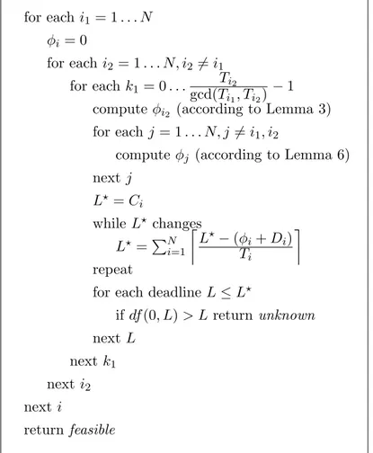
. The pseudo code for M = 2 is given in Figure 3.6.
3.4. ALGORITHM 25 for each i1 = 1 . . . N φi = 0 for each i2= 1 . . . N, i2 6= i1 for each k1 = 0 . . .gcd(TTi2 i1, Ti2) − 1
compute φi2 (according to Lemma 3)
for each j = 1 . . . N, j 6= i1, i2
compute φj (according to Lemma 6) next j L? = Ci while L? changes L? =PN i=1 » L?− (φi+ Di) Ti ¼ repeat
for each deadline L ≤ L?
if df (0, L) > L return unknown next L next k1 next i2 next i return feasible
3.5
Experimental evaluation
In this section, we evaluate the effectiveness of the proposed tests against Baruah’s sufficient synchronous test described by Theorem 1 and against the exponential test executed by checking the demand function for every dead-line until Φ + 2H. For each experiment, we generated 2000 synthetic task sets consisting of 6, 10 and 20 tasks, respectively, and with total utilization ranging from 0.8 to 1.
Each task set was generated in the following way. First, utilizations Ui were randomly generated according to a uniform distribution, so that the total utilization summed up to the desired value. Then periods were gener-ated uniformly between 10 and 200 and the worst-case computation time of each task was computed based on utilization and period. Finally, relative deadlines were assigned to be either between 0.3 and 0.8 times the task’s period or between half period and the period, and offsets were randomly generated between 0 and the period.
We experimented with two types of task sets. In the first case, we gen-erated the periods so that the greatest common divisor between any two tasks were a multiple of 5. In the second case, we chose the gcds as multi-ples of 10. The basic idea is that, if the gcd between two periods is 1, the distance between the release times of the two tasks can assume any value, 0 included. In the limit case in which all tasks’ periods are relatively prime, it is possible to show that the synchronous test is necessary and sufficient also for asynchronous task sets. Note that in the real world, a situation in which the task periods are relatively prime is not very common.
In each experiment we computed the percentage of feasible tasks using Baruah’s synchronous test, our test with one, two and three fixed tasks respectively, and the exponential test. In the following we will denote these tests with sync, 1-fixed, 2-fixed, 3-fixed and exponential, respectively. The results are presented in Figures 3.7, 3.8, 3.9, 3.10, 3.11, 3.12.
Figures 3.7, 3.8 and 3.9 shows the results for 6 tasks, with a minimum gcd of 10 in Figures 3.7 and 3.8 and a minimum gcd of 5 in Figure 3.9. In the first two figures, 1-fixed accepts a number of task sets up to 10% higher then the sync test. Performances are clearly lower with gcd = 5, as shown in Figure 3.9. Also note that the 2-fixed and 3-fixed tests do not achieve significant improvements over the 1-fixed test. In fact, increasing the number of fixed tasks seems to be beneficial only if the number of fixed tasks M is comparable to the number of total task N , but in that case the test obviously becomes not tractable (note that for M = N − 1 the test is
3.5. EXPERIMENTAL EVALUATION 27 0.8 0.82 0.84 0.86 0.88 0.9 0.92 0.94 0.96 0.98 1 0 0.1 0.2 0.3 0.4 0.5 0.6 total utilization
percentage of feasible task sets
synchronous 1 fixed task 2 fixed tasks 3 fixed tasks exponential
Figure 3.7: 6 tasks, gcd = 10, deadline ∈ [0.3, 0.8]T
0.8 0.82 0.84 0.86 0.88 0.9 0.92 0.94 0.96 0.98 1 0.2 0.3 0.4 0.5 0.6 0.7 0.8 0.9 1 total utilization
percentage of feasible task sets synchronous 1 fixed task 2 fixed tasks 3 fixed tasks exponential
synchronous 1 fixed task exponential
6 tasks 40 67 2233
10 tasks 122 387 461356
20 tasks 639 6341 42781200
Table 3.1: Mean number of cycles, gcd = 10, deadline ∈ [0.3, 0.8]T equivalent to the exponential one). The same considerations can be applied to Figures 3.10 and 3.11 where we show the results for 10 tasks and gcd = 10. The 1-fixed test again achieves very good results. For high computational loads, the improvement over the sync test is more than 10%. The 2-fixed and 3-fixed tests seem even less beneficial. The same holds in Figure 3.12 for 20 tasks and gcd = 10.
We also computed the mean number of simulation cycles needed to test a task set. Table 3.1 shows the results for gcd = 10 and deadline between 0.3 and 0.8 times the period for the sync, 1-fixed and exponential test. Notice that the number of cycles needed for the 1-fixed test is only one order of magnitude greater than the sync test. As the number of tasks increases we can appreciate that the growth in the number of cycles for the 1-fixed test is still acceptable compared to the corresponding growth of the exponential test.
3.6
Conclusions
In this chapter, we presented a new sufficient feasibility test for asynchronous task sets and proved it correct. Our test tries to take into account the offsets by computing the minimum distances between the release times of any two tasks. By analyzing a reduced set of critical arrival patterns, the proposed test keeps the complexity low and reduces the pessimism of the synchronous sufficient test. We showed, with an extensive set of experiments, that our test outperforms the synchronous sufficient test.
As future work, we are planning to extend our test to the case of relative deadline greater than the period.
3.6. CONCLUSIONS 29 0.8 0.82 0.84 0.86 0.88 0.9 0.92 0.94 0.96 0.98 1 0 0.05 0.1 0.15 0.2 0.25 0.3 0.35 0.4 0.45 0.5 total utilization
percentage of feasible task sets
synchronous 1 fixed task 2 fixed tasks 3 fixed tasks exponential
Figure 3.9: 6 tasks, gcd = 5, deadline ∈ [0.3, 0.8]T
0.8 0.82 0.84 0.86 0.88 0.9 0.92 0.94 0.96 0.98 1 0 0.1 0.2 0.3 0.4 0.5 0.6 0.7 0.8 total utilization
percentage of feasible task sets
synchronous 1 fixed task 2 fixed tasks 3 fixed tasks exponential
0.8 0.82 0.84 0.86 0.88 0.9 0.92 0.94 0.96 0.98 1 0.4 0.5 0.6 0.7 0.8 0.9 1 total utilization
percentage of feasible task sets synchronous 1 fixed task 2 fixed tasks 3 fixed tasks exponential
Figure 3.11: 10 tasks, gcd = 10, deadline ∈ [0.5, 1.0]T
0.8 0.82 0.84 0.86 0.88 0.9 0.92 0.94 0.96 0.98 1 0.75 0.8 0.85 0.9 0.95 1 total utilization
percentage of feasible task sets synchronous 1 fixed task 2 fixed tasks 3 fixed tasks exponential
Chapter 4
Resource usage extension
4.1
Introduction
In the previous Chapter 3, we developed sufficient schedulability tests for asserting the feasibility of asynchronous task sets under EDF. However, no resource constraints have been considered. In this chapter, we will extend the 1-fixed task test to cover the problem of resource usage.
The same task model as in the previous chapter is considered, but tasks are assumed to share resources as described in Section 2.1.1
Different resource access protocols have been proposed to bound the maximum blocking time of tasks due to mutual exclusion under EDF. We base our discussion on the Stack Resource Protocol proposed by Baker [2], which is the most frequently used. Under SRP, each task is assigned a static preemption level πi= 1
Di. In addition, each resource ρk is assigned a static
ceiling ceil(ρk) = maxi{πi|∃j, ρij = ρk}. A dynamic system ceiling is then defined as follows:
Πs(t) = max({ceil(ρk)|ρkis busy at time t} ∪ 0)
The scheduling rule is the following: a job is not allowed to start execu-tion until its priority is the highest among the active jobs and its preempexecu-tion level is strictly higher then the system ceiling.
Among the many useful properties of SRP, we are manly interested in two of them:
Property 1 Under SRP, a job can only be blocked before it starts execution;
once started, it can only be preempted by higher priority jobs.
Property 2 A job can only be blocked be one lower priority job.
In the following Section 4.2 we will introduce our modified test and prove it correct, while in Section 4.3 we will show how to compute a bound on the length of the busy period when resources are taken into account. The proposed analysis follows the one provided in [23].
4.2
Test extension
In order to prove our modified test, we now need to introduce some prelim-inary concepts.
Lemma 7 Given two tasks τi and τj, the minimum time distance between
any release time of task τi and the successive release time of task τj that is
greater or equal to some value q + 1 is equal to:
∆qij = φj− φi+l φigcd(T+ q + 1 − φj j, Ti)
m
gcd(Tj, Ti)
Proof. The proof is a simple extension of Lemma 2; it is sufficient to see that the condition on q is equivalent to considering τi being released q time units later. 2
Definition 3 Given task set T0
i, we define the following dynamic
preemp-tion level:
πi(t) = min({πj|φ0j+ Dj ≤ t} ∪ 2)
Note that instead of the constant 2 we could have used any numeric value that is strictly greater than any possible system ceiling (2 is clearly ok since no task can have a preemption level greater than 1).
Definition 4 Given task set T0
i, we define the following dynamic maximum
blocking time:
Bi(t) = max({Cjk− 1|Dj > t + ∆φjk
ji ∧ ceil(ρjk) ≥ πi(t)} ∪ 0) We can now prove our theorem:
4.2. TEST EXTENSION 33 Theorem 4 Given task set T with U ≤ 1, if ∀ 1 ≤ i ≤ N, ∀ L ≤ L?:
df (0, L) + Bi(L) ≤ L
where L is an absolute deadline of task set T0
i and L? is the first idle time
in the schedule of T0
i, then T is feasible.
Proof. By contradiction. Consider the schedule generated by EDF. Sup-pose a deadline is not met for task set T . Let t2 be the first instant at which a deadline is not met, and let t1 be the last instant prior to t2 such that no job with deadline less than or equal to t2 is active at t1− 1. Note that following this definition the busy period [t1, t2) is the same as in Lemma 1 if there are no blocking times, since all tasks that execute inside [t1, t2) must be released at or after t1 and have deadlines at or before t2. We will call A the set of all such tasks.
If blocking times are introduced, then it is possible for a single job τjp with deadline greater than t2 to be executed inside [t1, t2). For this to be possible, the job must be inside a critical section at time t1, since it must block some other job in A. Note that there can be only one such job; otherwise some job in A would be blocked by two lower priority jobs, which is impossible due to Property 2.
Now consider job τjp. Since it is inside a critical section at t1, it must hold ajp+ φjk < t1 for some k, and ajp+ Dj > t2 since its deadline is greater than t2. Now, there is surely a task τi that is release at t1. If the above conditions can hold, than they surely hold if we choose t1 − ajp = ∆φjk
ji , since it is the minimum possible time difference. Note that in any case the maximum blocking time induced by critical section ξjk is equal to Cjk− 1, since τjp can always be delayed by other tasks so that it enters ξjk at t1− 1. τjp must also be able to block some job in A, thus ceil(ajk) must be at least equal to the minimum preemption level of tasks in A. This proves that
Bi(t2 − t1) is indeed the worst-case blocking time.
To end the proof, it suffices to note that if we ”pull back” all jobs in A as in Theorem 2, the resulting schedule is still unfeasible. In fact, the tasks in A do not change, while since the new deadline t0
2 is less or equal than t2, the maximum blocking time is greater or equal than before. Finally, note that a task τj is in A if and only if φ0j+ Dj ≤ t02, thus πi(t) is in fact the minimum preemption level of tasks in A. 2
4.3
Busy period length
Note that the recurrence over the length of the busy period for task set T0 i: L? = N X j=1 » L?− (φ0j + Dj) Tj ¼
is no longer valid when blocking times due are considered. In fact, a task
τj whose offset is greater than or equal to the maximum length computed in this way, may still contribute to the busy period by adding a blocking time. The recurrence must thus be modified by adding the blocking time contribution: L?= N X j=1 » L?− (φ0j+ Dj) Tj ¼ + B?j(L?) where B?i(t) = max({Cjk− 1|φ0j ≥ t ∧ ceil(ρjk) ≥ π?i(t)} ∪ 0) and πi?(t) = min({πj|φ0j < t} ∪ 2)
![Figure 3.7: 6 tasks, gcd = 10, deadline ∈ [0.3, 0.8]T](https://thumb-eu.123doks.com/thumbv2/123dokorg/5665227.71470/37.892.156.593.211.571/figure-tasks-gcd-deadline-t.webp)
![Figure 3.9: 6 tasks, gcd = 5, deadline ∈ [0.3, 0.8]T](https://thumb-eu.123doks.com/thumbv2/123dokorg/5665227.71470/39.892.156.600.211.570/figure-tasks-gcd-deadline-t.webp)
![Figure 3.12: 20 tasks, gcd = 10, deadline ∈ [0.5, 1.0]T](https://thumb-eu.123doks.com/thumbv2/123dokorg/5665227.71470/40.892.226.681.202.978/figure-tasks-gcd-deadline-t.webp)
![Figure 5.1: 5 tasks, deadline ∈ [0.5, 1.0]T](https://thumb-eu.123doks.com/thumbv2/123dokorg/5665227.71470/54.892.225.742.175.603/figure-tasks-deadline-t.webp)
![Figure 5.2: 5 tasks, deadline ∈ [0.3, 0.8]T](https://thumb-eu.123doks.com/thumbv2/123dokorg/5665227.71470/55.892.153.668.171.601/figure-tasks-deadline-t.webp)