Issues in Environmental Economics: Sustainability and Eco-efficiency

Dipartimento di Scienze Economiche e Statistiche

Dottorato di Ricerca in Economia del Settore Pubblico

(XIII Ciclo – Nuova Serie)

Tesi di Dottorato

Issues in Environmental Economics:

Sustainability and Eco-efficiency

Coordinatore

Prof. Sergio Pietro Destefanis

Relatore

Candidata

Prof. Sergio Pietro Destefanis

Dott.ssa Maria Carmen Papaleo

Issues in Environmental Economics:

Sustainability and Eco-efficiency

Introduction

First Essay

Eco-efficiency, Energy and Air pollution: a NUT 3 analysis for Italy

1. Introduction

2. Defining eco-efficiency

3. The institutional set-up

3.1. The measurement of efficiency

4. The econometric set-up

4.1 The econometric model

4.2 The data

5. The econometric evidence

Concluding remarks

References

Second Essay

How much land does it take to support each person?

The Ecological Footprint and the Sustainability

1. Introduction

2. Ecological Footprint

3. Methodology

4. Carrying capacity and growth rate of population

5. Data analysis in Europe

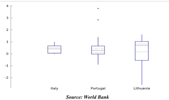
5.1 Growth rate of population

5.2 Urban population

5.3 Rural population

5.4 CO

emissions

6. Results and Conclusions

References

Sitography

Third Essay

Methane emissions and rice production: evidence from a large set of countries

1. Introduction

2. Data collection and methodology

3. Results

This thesis deals empirically with various research questions in environmental

economics. In particular the issues of sustainability and eco-efficiency are approached on

three different data-sets. The first paper deals with the analysis of eco-efficiency for 103

provincial (NUTS 3 - Nomenclature of Units for Territorial Statistics 3) capitals of Italy

throughout 2000-2008. It focuses on the link among economic growth, energy consumption

and air pollution, modeling cities as territorial units that ought to promote growth, while at

the same time minimising its environmental impact. Subsequently, the eco-efficiency of this

panel of provincial capitals is measured through panel estimates of an input-distance

function. Within this procedure, considering some environmental control variables, the

paper evaluates if environmental best practices correspond either to those municipalities that

adopt environment-friendly policies or to cities characterised by a particular urban context.

The evidence points to the existence of a significant link between economic development,

energy consumption and air pollution at the provincial capital level. The most ecoefficient

provincial capitals are also among the wealthier, which is consistent with an Environmental

Kuznets Curve.

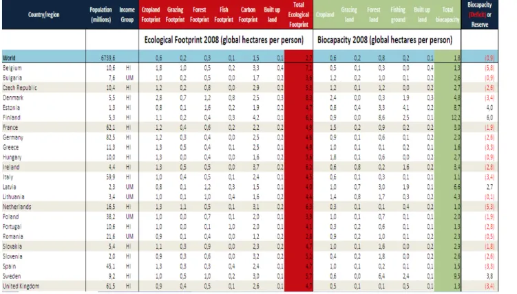
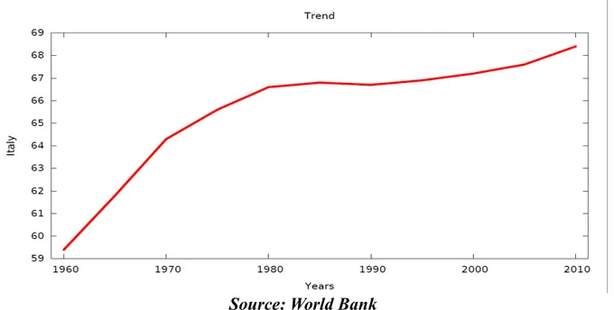
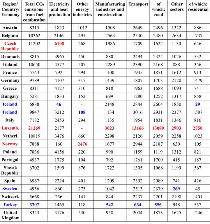
The second paper investigates the Ecological Footprint indicator by focusing on the

notion of sustainable development and then of carrying capacity of land. The impact of man

on nature is explored through an empirical analysis of the growth rate of population, and the

percentage of urban and rural population, in Europe. The level of CO

emissions per

inhabitant in the EU is compared with that of developing countries. Through a sectoral

approach, the total CO

emissions per capita from fuel combustion, electricity and heat

production, manufacturing industries and construction, transport and other sources are

separately appraised.

The third paper studies the relationship between rice production and methane

emissions. Rice farming is believed to be a major anthropogenic source of methane

emissions, which are measured emissions at both country and world levels of aggregation. It

presents a quantitative estimation of the statistical relationship between rice production

dynamics and methane emissions with regression estimates computed (country-wise and

globally) over a large set of countries. The evidence only partly validates the expectation of

a positive statistical influence of rice production on methane emissions. In fact a

Eco-Efficiency, Energy

and Air pollution:

Eco-Efficiency, Energy and Air pollution: a NUTS 3

analysis for Italy

Abstract

The aim of this paper is the analysis of ecoefficiency for 103 provincial (NUTS 3 -Nomenclature of Units for Territorial Statistics 3) capitals of Italy throughout 2000-2008. We focus on the link among economic growth, energy consumption and air pollution, modeling cities as territorial units that ought to promote growth, while at the same time minimising its environmental impact. Subsequently, we empirically assess the eco-efficiency of this panel of provincial capitals and, considering some environmental control variables, we evaluate if environmental best practices correspond either to those municipalities that adopt environment-friendly policies or to cities characterised by a particular urban context. Estimation is carried out through a parametric input-distance function. Our results confirm the existence of a significant link between economic development, energy consumption and air pollution at the provincial capital level. The most eco-efficient provincial capitals are also among the wealthier, providing evidence consistent with an Environmental Kuznets Curve. On the other hand, evidence in favor of a role of environment-friendly policies is insignificant.

Keywords: eco-efficiency; energy use; environment-friendly policy; air pollutants; Kuznets curve.

1. Introduction

The leitmotif of sustainable economic policies is to protect and to enhance the environment in the process of economic development for the benefit of a greater economic and environmental efficiency. In this paper we deal with these issues analysing the eco-efficiency of 103 Italian provincial capitals (the province being a NUTS 3 Nomenclature of Units for Territorial Statistics 3 -territorial jurisdiction, akin to a British county) throughout the 2000-2008 period. The motivation for this territorial level of analysis comes from the increasing importance taken by the concept of sustainability with respect to the issue of urban growth. Urban areas are increasingly becoming a nodal space within the global economy, in fact the city is an important generator of: wealth, employment opportunities, productivity growth, and a driving force for each national economy. At the same time, the city is also a generator of strong environmental pressures. So, the concept of urban eco-efficiency attracts attention and assumes a central role in analysis and policy evaluation.

The paper proceeds as follows. In the next section we deal with the definition of eco-efficiency, and subsequently with the construction of a function within the economic-environmental and economic territorial systems. The construction of an "environmental function" must have as its objective the rationalization in the use and management of natural resources and the preservation of the environment in connection with economic objectives related to the idea of development, and not in conflict with that. Economy and environment are closely interconnected with each other just like it is possible to see in the concept of sustainable development. Sustainable development is “development that meets the needs of the present without compromising the ability of future

generations to meet their own needs” (Bruntland Report, 1987).

In the third section we describe our institutional set-up. As we want to evaluate whether the best environmental practices correspond to those provincial capitals that have adopted

environment-choice of production set and measures of efficiency. The fifth section sets out the empirical counterpart of this approach, describing our data-set. The sixth section presents a comparative analysis of our regression results for various models (Not-per capita and Per capita models). Some concluding remarks are offered in the last section.

The fundamental contribution of Fare et al. (1989) analysed the harmful effects of the observed activities on the environment, taking into account the presence of undesirable outputs of the economic processes (output-environmental perspective) using econometric techniques. In particular, the most significant contributions are: Fare et al. (1989), Fare et al. (1993), Ball et al. (1994), Lovell et al. (1995).

An alternative to the classical approach is adopted by the input-environmental literature. This consists in including environmental harmful inputs in the set of production possibilities, in order to assess the environmental effects of bad inputs (input- environmental perspective). In this strand of the literature, the most significant contribution is the approach of Reinhard (1999). An alternative approach to the Reinhard (1999) model is the work of Kortelainen and Kuosmanen (2004b).

2. Defining eco-efficiency

In general terms, eco-efficiency is the optimal use of resources compatibly with the environment and involves minimizing environment-damaging while maximizing the economic outcome of production processes. Eco-efficiency reflects the capacity of a given unit (a firm, a territorial area, etc.) to transform inputs in outputs in an optimal way with respect to a benchmark, while considering at the same time also the environmental impact, through more recycling, lesser use of energy and natural resources, elimination of dangerous emissions. The definition of eco-efficiency hence naturally considers both economic and environmental parameters.

In the case of territorial systems, the areas of application of the eco-efficiency concept can be different: transport, greenhouse gases emissions and air pollution, waste, water, the share of renewable energy, investments for environmental protection. In this paper we refer to the eco-efficiency of the provincial capitals of Italy with respect to a series of environmental variables referring to energy consumption and air pollution. We model cities as territorial units that are assumed to promote economic development, while at the same time minimizing its environmental impact in terms of energy consumption and air pollution.

Urban areas are increasingly becoming a nodal space within the global economy. All along history, one of the main functions of the city has been its ability to catalyse economic activities and attract population. The city is an important generator of wealth, employment opportunities, productivity growth, and a driving force for each national economy; at the same time, the city is also a generator of strong environmental pressures. Cities in fact produce a significant part of a country GDP and, in most cases, large cities per capita GDP is higher than the national average. Cities gather half of the world population, even if they occupy only 2% of the Earth's surface, using 75% of the natural resources of the world (UNDP, 2003). However, this acceleration of urbanization in the world, albeit strengthening the economic importance of the city, and causing the concentration of population, economic activities, social and leisure facilities in the cities themselves, also generates a continuous pressure on the surrounding environment with negative externalities (OECD, 2006). For this reason, it is necessary to make cities drivers of the local economy in an environmentally sustainable manner.

Our paper proposes an econometric analysis of the features of urban environmentally sustainable growth, focusing on the economic and environmental performance of the provincial

capitals of Italy, as far as energy consumption and air pollution are concerned. We aim to assess whether environmental best practices correspond either to those municipalities that adopt environmentally sustainable policies or to cities characterized by a particular urban context. One question we want to answer in this paper is if the most economically developed cities of the Italian economy have become, in the course of time, also the most environment-friendly or have, on the contrary, paid their development in terms of environmental damage. We rely on a large data-set, mostly based upon official data, covering 103 provincial capitals of Italy throughout the 2000-2008 period.

3. The institutional set-up

The aim of our research is the analysis of eco-efficiency for the provincial (NUTS 3) capitals of Italy. The Nomenclature of Units for Territorial Statistics (for French “Nomenclature des unités

territoriales statistiques”) is a standard geocode (3 is for provinces). More information about the

Italian provinces is provided in Appendix A (see Figure A.1 in particular). We want to evaluate the economic and environmental performance of provincial capitals in a sustainable development perspective, in order to identify eco-friendly capitals adopting an effective and efficient political-environmental governance. Therefore, focusing on the link between economic development and its environmental impact in terms of energy consumption and air pollution, we assess the 2000-2008 period to gauge whether environmental best practices correspond to those provincial capitals that they have adopted environment-friendly policies (detailed below) or to cities characterized by a particular urban context, from an economic or territorial point of view (presence of industries, weather-climate situation, population density).

The empirical basis for our investigation is constituted by the annual provincial data for 103 provincial capitals of Italy, on a time span ranging from 2000 to 20081_{. Our attention is focused on}

urban centres as the main actors in a model of sustainable development. In fact, they are important generators of wealth, opportunities of employment and productivity growth, but at the same time they are also strong generators of environmental pressures.

We now proceed to describe the set of environment-friendly policies that is of interest for our purposes (PEC and PUT). PEC stands for Piano Energetico Comunale (Municipal Energy Plan). Law no. 10, 1991 includes an obligation for municipalities with population of more than 50,000 inhabitants to prepare an Energy Plan. This Plan seeks to identify strategic guidelines in the energy sector, to verify the existence of conditions and resources for their implementation and to monitor over time their effective implementation. PUT stands for Piano Urbano del Traffico (Urban Traffic Plan). It is an administrative tool "aimed to obtain the improvement of traffic conditions and road safety, the reduction of noise and air pollution and saving energy, in agreement with the existing urban instruments and transport plans, and with respect for environmental values, establishing the priority and timing of implementation of the interventions. The urban traffic plan resorts to appropriate technological systems on the information basis of traffic regulation and control, as well as verification of the slowdown in speed and parking deterrence aimed also to allow changes to the traffic flows that they may be required with respect to the objectives to pursue" (Art. 36, Legislative Decree no. 285, 1992). The adoption of PUT is mandatory for municipalities with a resident population of more than 30,000 inhabitants. PUT should be updated every two years to adapt it to the general objectives of the socio-economic and territorial planning.

3.1 The measurement of efficiency

Currently, the issue of sustainability, especially at the local level, concerns the relationship between economic growth and environmental protection in terms of containment of polluting emissions generated by anthropogenic activities. Subsequently, we jointly consider the economic and environmental performances of the provincial capitals of Italy. Each human activity gives rise to a joint production of desirable and undesirable outputs obtained by the application of an input set. Hence the first step toward the measurement of efficiency in our analysis is the specification of the relevant inputs, good outputs and bad outputs for the provincial capitals of Italy. We assume that the main function of urban centres with an institutional and socio-economic importance is their attractor function for population and economic activities. Concentration of population and their activities generate economic development, but also determine strong environmental pressures. We model this in the following manner.

We take as good outputs (good Y), population, as a proxy of employment opportunities, and bancarization (the sum of banking loans2 _{divided by the resident population), as an income proxy.}

This choice of proxies is essentially dictated by considerations of data availability.

In addition to these good outputs, our model incorporates some bad outputs: the environmental-damaging variables. Our undesirable output (bad Y) will consist of environmental pressures due to atmospheric emissions resulting from human activities in the phase of consumption (energy consumption and transport in particular), since the greater environmental impact at the local level is determined by the resident consumption. It is estimated that about 75% of the Italian population lives in urban areas where it consumes more than 70% of energy and from where it comes more than 80% of anthropogenic emissions of greenhouse gases. The incidence of this phenomenon allows to measure the economic development and social cohesion policies, the sustainable strategies and actions by the cities, and the global challenges of the struggle against climate change3 _{(ISPRA, 2008). The decision to focus on anthropogenic pressures in the}

consumption phase, and not also in the production phase, mainly derives from the availability of the relevant data. Yet, consider that the major environmental pressures at the municipal level are generally ascribable for 40% to the residential sector, 35% to transport and only for 20% to industry (Cittalia-ANCI, 2010). In our particular case, therefore, we consider the environmental pressures with respect to air pollution derived from two sources of pollution: road transport and residential energy consumption. More precisely, the negative environmental pressures to the atmospheric level that we will consider in our empirical analysis are: PM10 surpluses4, methane gas consumption and electricity

consumption. The latter are proxies for CO2 emissions that contribute to global warming. We would

like to have measures of other fuel consumption, or, even better, direct measures of CO2 emissions,

but data of this kind are not readily available.

Obviously, cities are supposed to maximize good Y, while at the same time minimizing bad Y

and inputs. There has not been so far any reference to a conventional input, and there will not be

any. In fact, in accordance with the hypothesis of Lovell et al. (1985), we assume that each provincial 2 _{A more usual definition of the bancarisation index is the sum of banking loans and deposits, divided by the}

resident population. We tried in estimation both definitions and retained the more significant one.

3 _{Climate change is determined by anthropogenic activities and it is generated by gas greenhouse effect. The}

main GHG (greenhouse gases) associated with global climate change, are: CO2 (carbon dioxide), CH4

(methane), N2O (nitrous oxide), CO (carbon monoxide). Currently, climate experts predict a trend to the

acceleration of the changes in temperature and that the average temperature will increase by 2100 of 1.4°-5.8°C globally and by 2°-6.3°C at the European level.

4 _{This indicator is the number of days when PM}

10 emissions were above their warning level in the municipal

capital has a fixed-amount capability “to be a provincial capital” (the so-called “ability of the helmsman”, supposed as fixed for each unit of analysis, and modeled as a constant term).

Finally, the ability to transform inputs into good Y, while at the same time minimizing bad Y can be affected by given policies as well as the type of “urban environment”. Such control or context variables (Z) will also be included in our production set, as they have an influence on the economic and environmental performances of the different territorial units. We consider the following Z variables: the eco-friendly policies (PEC, PUT), the local temperature (lowest, highest and average temperatures), the population density and the share of industry (local employment in industry over total local employment)5_.

The relationships singled out by our model of the environmentally sustainable production process of the Italian provincial capitals of Italy are displayed in Figure 3.1.

Figure 1: Environmentally Sustainable Production Process of Italian Provincial Capitals.

After having defined the production set, we need to proceed to a suitable definition of efficiency. We consider a very general concept of eco-efficiency: the relationship between inputs and outputs compared with a benchmark of optimality, also allowing for the environmental impact of the production process (this broad definition is consistent with a very large literature: Reinhard et al., 1999; Kortelainen and Kuosmanen, 2004a, 2004b; Nissi and Rapposelli, 2005; Zhou et al., 2008). As hinted above, cities are then supposed to maximize good Y, while at the same time minimizing bad Y

and inputs. Best-practice cities will be defined as efficient, and underperforming cities as inefficient.

In our analysis we make two important choices: we rely on a parametric frontier approach, and model bad outputs as inputs. The motivation for the first choice mainly comes from the desire to take advantage of the panel structure of our data (more details about this are of course provided below) to deal with unobserved heterogeneity, as well as from the need to allow in the analysis for a rather rich set of control variables. The second choice, which takes the cue from some previous

studies (Korhonen and Luptacik, 2004; Growitsch et al., 2005), comes from the idea that cities aim to minimise environment-damaging variables in the same manner as inputs must be usually minimized in the analysis of productive efficiency. Using this simplifying hypothesis should not be misleading when considering the outcome of aggregated decisions (as we are doing at the city level), and, as shown in Growitsch et al. (2005), lends itself straightforwardly to the parametric analysis of efficiency. Given this assumption, provincial capitals will be (eco-)efficient if they maximize their good outputs for a given level of bad outputs, or, conversely, if they minimize their bad outputs for a given level of good outputs (naturally, the control variables will impinge upon this process, and must be duly allowed for).

4. The econometric set-up

4.1 The Econometric Model

Once we have identified the variables of our production set, in order to bring this model to the data, we need to specify for it an appropriate functional form.

Summing up, our production set includes two (good) outputs: population (Y1) and the index

of “bancarization” (Y2); three proxies (modeled as inputs) of the atmospheric environmental

pressures represented by PM10 surpluses (P1), methane gas consumption (P2), electricity

consumption (P3); seven control variables: eco-policies “PEC” (Z1), “PUT” (Z2); the mean, highest and

lowest local temperature (Z3, Z4 and Z5), population density (Z6) and the industry share (Z7).

We choose to model this production set econometrically through an input distance function, similar to the one in Growitsch et al. (2005), and we estimate it through a panel fixed-effect model, including idiosyncratic time trends for each provincial capital. The inclusion of these trends allows for existence of time-varying efficiency in the production process. This is a very important point because it allows measurement of the eco-efficiency over time, while most existing empirical studies in the eco-efficiency literature use cross-sectional data. Reliance on panel data allows to investigate the changes in performance and efficiency over time, as well as to deal successfully with the possible correlation between efficiency terms and regressors.

In general terms the distance function can be written as:

f (y1, y2)= f (p1..., pn, z1... zn) + εit (1)

where the y represent the conventional outputs, the p the environment-damaging proxies (modelled as inputs), and the z the control variables that affect the production process of the local systems. This is our baseline model.

Following common practice, we now assume a translog functional form for the input distance function

y

x

x

x

x

y

y

y

D

l n

l n

2

1

l n

l n

2

1

l n

l n

l n

2

1

l n

l n

 

 

































Imposing suitable restrictions (homogeneity, symmetry and monotonicity), the translog distance function can be specified as follows:

i t m i K I k i k m K i l i K I k i k l i K k i K = k k n i m i m n M = n M = m m i M = m m 0 K i

u

y

x

x

δ

+

x

x

x

x

β

+

x

x

β

+

y

y

α

+

y

α

+

α

=

)

( x

















l n

l n

2

1

l n

l n

2

1

l n

l n

l n

2

1

l n

l n

Where the u terms stands for inefficiency, and for the sake of generality we opt for a model with no input-output separability. Following the literature, the translog distance function becomes, in presence of panel data with time-varying efficiency:

m i t K i t k i t k m K i t l i t K i t k i t k l K i t k i t K = k k n i t m i t m n M = n M = m m i t M = m m i t K i

y

x

x

δ

+

x

x

x

x

β

+

x

x

β

+

y

y

α

+

y

α

+

α

=

)

( x

l n

l n

2

1

l n

l n

2

1

l n

l n

l n

2

1

l n

l n















Where t = 1, ...,T, are time periods and, as shall be explained below,

it t it  u

 . In our

empirical analysis, we extend this model through the inclusion of the control variables, z:

sit s S = s s 0 i

=

λ

+

λ

λ

z

m

ln



in order to allow for their role in the determination of eco-efficiency.

As already said, we estimate this function through a panel fixed-effects model under the hypothesis of efficiency variability over time. Once singled out the best practice frontier from the multi-input multi-output translog input distance function model we compute the efficiency scores as deviations from this frontier. Following Cornwell et al. (1990), we estimate coefficients

, , , ,   

and technical efficiency through a within estimator. In this model each provincial capital has its own intercept, that changes over time according to a linear trend with unit-specific time-variation coefficients. The technical inefficiency of a provincial capital in a particular period is obtained from the estimated intercepts through a normalization operation.

The time-variation structure is the same for each

it

α and is specified as:

it i it  'z   (6) where: i

 = vector of time-variation coefficients of individual intercepts

_z

₍

₁

_,

_t

_,

_t

₎

it



t

θ

+

θ

+

θ

=

α

Note that the time-variation pattern becomes specific for each provincial capital, because coefficients vary across them. After estimating

it

α , the normalization operation is carried out, finally obtaining:

 







max

u









3.4.2 The data

Subsequently to our definition of inputs and outputs, we construct a panel data-set (through 2000-2008) for 103 Italian provincial capitals, mainly based upon the Indicatori Ambientali Urbani data-set of Istat). In particular, we recover the data from the following sources:

 The Indicatori Ambientali Urbani - Urban Environmental Indicators (ISTAT)6 _for

environment-damaging proxies (PM10 surpluses, and residential energy

-methane gas and electricity - consumption), and for some control variables (PEC, PUT, industry share, population density);

 The Andamento meteo-climatico in Italia – Weather and Climate Trend in Italy (ISTAT)7 _{for the context variables related to local temperatures (lowest, highest}

and mean local temperatures);

 The Atlante Statistico dei Comuni - Statistical Atlas of Municipalities (ISTAT)8 _for

the population and the bancarisation variables (for 2008, this information was complemented by data from the Bollettino Statistico - Statistical Bulletin; Bank of Italy);

 The Sistemi locali del lavoro (Local Labour Systems) database from ISTAT9 _{for the}

industry share.

Summing up, all the data are at provincial capital level, but for the industry share, which is measured at the local labour system level. In the construction of the data-set, the main problem was to integrate the missing data of the PM10 surpluses. For this purpose we adopted an imputation

procedure based upon the MCMC method (Cameron and Trivedi, 2005)10_{, to complete the series}

with the imputed values of PM10 from 2000 to 2002 for all territorial units and in some cases for other

years, where it was necessary. In this imputation procedure we used as regressors the PM10

surpluses of the following two years, the motorisation rate, and the local lowest temperature. However, for seven provincial capitals (Chieti, Foggia, Crotone, Cosenza, Catanzaro, Trapani, Ragusa) it was not possible to make any imputation for the total missing data.

For the electricity measures, we computed total consumption of electricity multiplying the 6 _{http://www.istat.it/it/archivio/67990}

7 _{http://www.istat.it/it/archivio/5679} 8 _{http://www.istat.it/it/archivio/113712}

9 _{http://www.istat.it/it/archivio/sistemi+locali+del+lavoro. The Sistemi locali del lavoro (Local Labour Systems)}

are groups of municipalities (akin to the UK’s Travel-to-Work-Areas) adjacent to each other geographically and statistically comparable, characterised by common commuting flows of the working population. They are an analytical tool appropriate to the investigation of socio-economic structure at a fairly disaggregated territorial level.

10 _{For an application of this technique to the imputation of missing values when measuring efficiency in the}

public sector, see Destefanis and Ofrìa (2009). This imputation obtains estimates of the missing values by regressing the variables of interest (for the available observations) on some correlated variables that, for the

per-person values provided by ISTAT (kwh for inhabitant) by the resident population. The same applies to the methane consumption: after excluding four provincial capitals whose gas measures are non-existent or abnormal (Nuoro, Oristano, Reggio Calabria, Sondrio), we calculate total gas consumption multiplying the ISTAT per capita values (m³ per capita) by the resident population.

3.5. The econometric evidence

We now take our model to the data11_{. To repeat, our sample is composed of 103 provincial}

capitals observed from 2000 to 2008: the total number of observations is therefore of 927 observations, being a balanced panel. We already stressed that the panel nature of our analysis allows us to deal with changes in the efficiency levels. More particularly, we consider here the hypothesis of time-varying efficiency, both through idiosyncratic time trends and the influence of context variables changing over time.

In order to better evaluate eco-efficiency and its variations over time, in addition to the baseline model (also to labelled below as the Not-per capita model), we analyse an additional model for purposes of comparison, a Per capita model12_{. The Per capita model considers only one output}

(bancarisation) and takes all the bad outputs in terms of per capita variables. In fact, the baseline Not-per capita model should be in principle more informative, allowing us to measure the eco-efficiency in a more articulated way. However, we have observed some anomalies in its results, suggesting the advisability of further comparisons. The choice to rely upon the Per capita model stems from the possibility (to be expounded below) that there are measurement problems linked to population growth.

All the three models are estimated through the input distance function with fixed-effects and idiosyncratic time trends for each provincial capital (we finally relied upon a linear time trend specification, as the quadratic term was not significant).

Table 3.1: Specification of Not-per capita, Per-capita and Without PM10 models.

VARIABLES Not-per capita Per capita Without PM10

Good Outputs

Population X X

Bancarisation X X X

Bad Outputs (Inputs)

PM10 surpluses X X

Gas consumption X X X

Electricity consumption X X X

Control Variables

PEC X X X

11_{The econometric analysis is carried out through STATA 12.}

12 _{We also estimated a Without PM10 model, not considering the PM10 surpluses among the bad outputs. This}

Without PM10 model finds its justification in the problems of data collection about this pollutant. We wanted to

Table 3.2: Specification of Not-per capita, Per-capita and without PM10 models.

VARIABLES Not-per capita Per capita Without PM10

PUT X X X

Local temperatures X X X

Population density X X

Industry share X X X

Note: in this model not only bancarisation, but also the bad outputs are expressed in per capita

terms.

We will now present the main results of the estimates (the detailed results are provided in Appendix A). Broadly speaking, we find that the translog distance function seems to work well. There is a significant link between economic development, energy consumption and air pollution at the provincial capital level, and the input and output coefficients have the right signs. The evidence from the Not-per capita and Per capita models ranks is broadly compatible, also as far as the lack of significance of the policy variables and the other controls is concerned. None of the latter turns out to be significant. In the estimates reported in Appendix A, we want to highlight the scant role played by the eco-friendly plans (PEC and PUT). To verify the relevance of eco-plans in the process of city and eco-efficiency development, we considered not only intercept dummies but also trend dummies for PEC and PUT. We never found significant values for these variables. There was even some evidence (see Table A.1) of PEC coming out with the “wrong” sign.

An important point is that we do not want to rely, when interpreting the evidence, upon fixed effects that are affected by many unobserved geographical and institutional (fixed) factors. This leads us to consider only time-varying eco-efficiency in our following comments. In Appendix B, we report in detail the results for the idiosyncratic efficiency trends, all provinces departing from a conventional value of 100 for year 2000. We also single out some best practices, labeling as eco-efficient the municipalities that have in 2008 a score above the value of 101 for the Not-per capita model and above the value of 104 for the Per capita model.

As shown in Figure 3.2, the 2008 eco-efficiency values from the Not-per capita and Per capita models are pretty close.

Figure 2: Not-per capita and Per capita Eco-efficiency, 2008.

Not-per capita model must be preferred for its goodness of fit, perusal of the results elicits some perplexities about this model. For some observations, e.g. in Naples and Bologna, the eco-efficiency results of the Not-per capita model are not confirmed in the Per capita model. This leads us to speculate that the Not-per capita model may be affected by some distortions. Arguably population is connected to some relevant institutional factors such as the substitution by methane of other fuel. A larger population is likely to be correlated with a larger users/population ratio for methane gas, and a with a smaller users/population ratio for other fuel. The neglect of this important link creates a measurement error for population and gas consumption that affects estimation of our baseline model. The data at our disposal not allow, however, to take account of the substitution of other fuel by methane in the provincial capitals. Hence, even if the Not-per capita model makes more econometric sense (it has higher goodness of fit), we prefer to draw our final comments of the evidence mainly referring to the Per capita model.

Indeed, from the comparative analysis in Appendix B of our two models (Not-per capita and Per capita), it clearly appears that the Per capita ranking is more informative because it highlights not only the best practices, but also a more understandable regional pattern for these success cases. The best performers overwhelmingly show up in North-eastern Italy: Trentino Alto Adige, Emilia Romagna and eastern Lombardy, with two outsiders represented by Biella and Siena (yet Siena, the headquarter of the important Montepaschi bank, may have unduly benefited from the inclusion of the bancarisation among outputs). More in detail, the most eco-efficient provincial capitals of Italy are: Bergamo, Biella, Bologna, Bolzano, Brescia, Cagliari, Lecco, Naples, Parma, Piacenza, Reggio nell'Emilia, Sassari, Siena, Trento and Verona. The analysis of these best practices with respect to the energetic plans does not show so much (recall that the PEC is compulsory for the municipalities with at least 50,000 inhabitants and the PUT for municipalities with at least 30,000 inhabitants). However, it is also true two eco-efficient municipalities (Lecco and Biella) have adopted the PEC without it being compulsory for them. All in all, our analysis seems to imply that if a greater wealth implies more consumption and emissions, on the other hand more economic resources probably also allow the realization of eco-friendly policies that lead to a greater eco-efficiency. This would explain why the more eco-efficient Italian capital provinces belong to the more economically advantaged regions of Italy. This impression is validated by an exploratory statistical analysis. Table 3 below provides Spearman rank correlation coefficients for the level of eco-efficiency in 2008 Not-per capita and Per capita, the (natural log of the) provincial value added per capita (these are mean values for 2000-2007, taken from ISTAT territorial statistics), and a provincial index of social capital (taken from Santini, 2005). Notice that value added per capita and social capital are available for provinces, not provincial capitals.

Table 3: Spearman correlations among eco-efficiency and other variables

Not-per c. e.e. Per-c. e.e. y per c.

Per-c. e.e. 0.8258

y per c. 0.2890 0.4591

social K 0.1801 0.3296 0.7321

Clearly, there is a sizable correlation between our Not-per capita and Per-capita eco-efficiency measures (as well as between value added and social capital). Some correlation also emerges between eco-efficiency and the other indicators (especially value added per c.).

Yet, when allowance is made for the simultaneous influence of value added per c. and social capital over eco-efficiency, correlation between the later and social capital apparently

regressions (Verardi and Croux, 2009) including the above considered variables that rather support this story.

Table 4: Robust regressions among eco-efficiency and other variables

Non-per c. Eco-eff. on y per c., social K

Coeff t-ratio

y per c. 8.778637 2.11

social K -13.29471 -0.83

pseudo-R sq 0.04

Per-c. Eco-eff. on y per c., social K

Coeff t-ratio

y per c. 15.34428 4.37

social K -3.466137 -0.21

pseudo-R sq 0.19

The above results (strongly supported by standard OLS regressions, available upon request) are of course consistent with the approach of the Environmental Kuznets Curve (for recent analyses of this approach, see Halkos and Tzeremes, 2013; Carillo and Maietta, 2014). Greater wealth is likely to bring about stronger claims for protection of the environment, and possibly to more environmentally sustainable behaviours. The results from Table 3.4 also validate our former contention to the effect that the Per-capita measure of eco-efficiency is much less noisy.

Concluding Remarks

In this paper we have analyzed 103 Italian provincial capitals over the 2000-2008 period. We find a significant link between economic development, energy consumption and air pollution at the provincial capital level. Also, if greater wealth leads to more energy consumption and pollution, on the other hand, greater economic resources probably also allow the creation of environmentally sustainable policies that lead to a greater eco-efficiency. Consistently with the approach of the Environmental Kuznets Curve, this would explain why the more eco-efficient provincial capitals of Italy belong to the more economically advantaged regions.

Our study naturally lends itself to further development and research. It would be interesting to put more emphasis on the decoupling between development and pollution that takes place in the richest regions by considering the consumption of various kinds of fuel. Moreover, it would also be interesting to assess the economic and environmental performance of the capitals of Italy taking into consideration the CO2 emission, dioxide carbon being the gas that most contributes to the climate

change (around 75% of global emissions of greenhouse gases) and therefore the target of reference of all international agreements on this field. At present, however, we believe that our study, although limited to residential energy consumption and to only one pollutant (PM10), provides a significant first

analysis of the links among development, consumption and air pollution emissions in urban areas of the provincial capitals of Italy.

APPENDIX A

Legend of Figure A.1: Legend of Province Abbreviations (in alphabetical order).

Abbreviation Province Abbreviation Province Abbreviation Province

AG Agrigento LI Livorno TP Trapani

AL Ale s sandria LO Lodi TN Trento

AN Ancona LU Lucca TV Treviso

AO Aosta MC Macerata TS Trieste

AR Arezzo MN Mantova UD Udine

AP Ascoli Piceno MS Massa-Carrara VA Varese

AT Asti MT Matera VE Venice

AV Avellino ME Messina VB Verbania

BA Bari MI Milan VC Vercelli

BL Belluno MO Modena VR Verona

BN Benevento NA Naples VV Vibo Valentia

BG Bergamo NO Novara VI Vicenza

BI Biella NU Nuoro VT Viterbo

BO Bologna OR Oristano BZ Bolzano PD Padova BS Brescia PA Palermo BR Brindisi PR Parma CA Cagliari PV Pavia CL Caltanissetta PG Perugia CB Campobasso PU Pesaro e Urbino

CE Caserta PE Pescara CT Catania PC Piacenza CZ Catanzaro PI Pisa CH Chieti PT Pistoia CO Como PN Pordenone CS Cosenza PZ Potenza CR Cremona PO Prato KR Crotone RG Ragusa CN Cuneo RA Ravenna

EN Enna RC Reggio di Calabria

FE Ferrara RE Reggio nell'Emilia

FI Florence RI Rieti FG Foggia RN Rimini FC Forlì-Cesena RM Rome FR Frosinone RO Rovigo GE Genova SA Salerno GO Gorizia SS Sassari GR Grosseto SV Savona IM Imperia SI Siena IS Isernia SR Syracuse SP La Spezia SO Sondrio AQ L'Aquila TA Taranto LT Latina TE Teramo LE Lecce TR Terni LC Lecco TO Turin

Table A.1: Regression Results for the Not-per capita and the Per-capita models

Not-per capita model ( dep. var.: - Lpm10_) Per-capita model ( dep. var.: - (Lpm10_ - Lpop_))in the Per-c. Model, all y's and p's are deviations from Lpop_

Var. Coeff. T-ratio Var. Coeff. T-ratio

Lbanc_ -0.035916 -2.36 Lbanc_ -0.046716 -4.03 Lpop_ -0.424270 -4.59 ~ bancq 0.008018 1.11 bancq 0.004327 0.59 popq 0.137141 4.44 ~ bancpop -0.007161 -0.38 ~ gas_pm10 0.133607 6.24 gas_pm10 0.139450 9.02 ele_pm10 0.858141 39.44 ele_pm10 0.855846 54.24 gas_pm10q 0.015856 3.26 gas_pm10q 0.018108 3.72 ele_pm10q 0.018617 3.48 ele_pm10q 0.017789 3.81 gas_ele -0.031356 3.37 gas_ele -0.035069 -3.94 gas_pm10_b~c 0.045464 2.79 gas_pm10_b~c 0.047303 3.66 ele_pm10_b~c -0.045283 -2.71 ele_pm10_b~c -0.050506 -3.88 gas_pm10_pop -0.009305 -0.55 ~ ele_pm10_pop 0.000712 0.04 ~ PEC_ -0.007001 -1.38 PEC_ -0.007890 -1.58 PUT_ 0.006368 0.93 PUT_ 0.007497 0.97 Tr1 0.009024 2.80 Tr1 0.010700 3.53 Tr2 0.011699 12.19 Tr2 0.015506 4.16 Tr3 0.004101 3.34 Tr3 0.000639 0.23 Tr4 0.001973 0.62 Tr4 -0.000021 -0.08 Tr5 0.002743 3.11 Tr5 0.004637 1.93 Tr6 0.000327 0.28 Tr6 -0.002432 -0.54 Tr7 0.012858 12.15 Tr7 0.011523 4.68 Tr8 -0.002158 -1.91 Tr8 -0.001439 -0.64 Tr9 0.008389 5.08 Tr9 0.006386 2.66 Tr10 0.012285 6.91 Tr10 0.010244 3.18 Tr11 -0.004719 -2.96 Tr11 -0.007006 -2.94 Tr12 0.016893 3.49 Tr12 0.017797 3.28 Tr13 0.023774 12.54 Tr13 0.020626 6.17 Tr14 0.016864 11.84 Tr14 0.013534 3.19 Tr15 0.036102 27.39 Tr15 0.038308 9.44 Tr16 0.020797 7.62 Tr16 0.019673 5.24 Tr17 0.000926 0.37 Tr17 -0.005128 -1.84 Tr18 0.021325 5.04 Tr18 0.013322 3.24 Tr19 0.001825 1.13 Tr19 -0.003712 -1.51 Tr20 -0.000102 -0.08 Tr20 -0.003165 -0.91 Tr21 0.005147 3.17 Tr21 0.006362 1.92 Tr22 0.011610 2.63 Tr22 0.001713 0.37

Not-per capita model ( dep. var.: - Lpm10_) Per-capita model ( dep. var.: - (Lpm10_ - Lpop_))in the Per-c. Model, all y's and p's are deviations from Lpop_

Var. Coeff. T-ratio Var. Coeff. T-ratio

Tr24 — — Tr24 ― — Tr25 0.006894 5.05 Tr25 0.008053 3.36 Tr26 — — Tr26 — — Tr27 0.011454 10.31 Tr27 0.009095 3.15 Tr28 — — Tr28 — — Tr29 0.009665 9.13 Tr29 0.008292 3.20 Tr30 -0.008722 -4.75 Tr30 -0.014355 -5.16 Tr31 0.007153 5.73 Tr31 0.005821 2.11 Tr32 0.005276 1.53 Tr32 0.004024 1.30 Tr33 — — Tr33 — — Tr34 -0.001812 -1.83 Tr34 -0.000489 -0.19 Tr35 0.002830 1.95 Tr35 -0.001211 -0.40 Tr36 0,014784 6,63 Tr36 0,010059 2,33 Tr37 0,014683 11,06 Tr37 0,010420 3,47 Tr38 0,003319 3,03 Tr38 0,007587 3,70 Tr39 0,009349 4,33 Tr39 0,007975 2,59 Tr40 0,001196 0,56 Tr40 -0,001780 -0,59 Tr41 -- -- Tr41 -- --Tr42 0,006873 7,98 Tr42 0,005505 1,70 Tr43 -0,008673 -6,65 Tr43 -0,006416 -2,12 Tr44 0,005450 4,46 Tr44 0,010356 1,93 Tr45 0,016875 10,92 Tr45 0,015618 4,19 Tr46 0,006474 4,96 Tr46 0.004630 2.17 Tr47 0.006690 3.22 Tr47 0.006638 1.35 Tr48 0.001595 1.24 Tr48 -0.000182 -0.07 Tr49 0.011593 7.26 Tr49 0.010917 3.94 Tr50 0.005213 2.57 Tr50 0.002129 0.71 Tr51 -0.000657 -0.58 Tr51 -0.001480 -0.34 Tr52 0.001636 1.80 Tr52 -0.000380 -0.10 Tr53 0.005160 2.22 Tr53 -0.002274 -0.60 Tr54 0.010044 1.96 Tr54 0.015036 2.82 Tr55 -0.004388 -2.49 Tr55 -0.004830 -1.73 Tr56 0.020406 8.82 Tr56 0.008907 3.06 Tr57 0.010740 11.34 Tr57 0.008358 4.30 Tr58 — — Tr58 — — Tr59 — — Tr59 — — Tr60 0.009125 4.56 Tr60 0.008498 2.80 Tr61 0.014653 5.55 Tr61 0.003586 1.05 Tr62 0.009310 5.81 Tr62 0.015795 5.75 Tr63 0.010382 8.48 Tr63 0.006227 2.29 Tr64 0.001856 1.39 Tr64 0.007630 2.01 Tr65 0.008334 7.65 Tr65 0.005464 1.57

Not-per capita model ( dep. var.: - Lpm10_) Per-capita model ( dep. var.: - (Lpm10_ - Lpop_))in the Per-c. Model, all y's and p's are deviations from Lpop_

Var. Coeff. T-ratio Var. Coeff. T-ratio

Tr66 0.005393 3.51 Tr66 0.005673 1.39 Tr67 0.015340 14.66 Tr67 0.016013 6.80 Tr68 -0.005210 -2.40 Tr68 -0.011918 -4.48 Tr69 0.001031 0.93 Tr69 0.001310 0.60 Tr70 0.014793 18.11 Tr70 0.013107 5.33 Tr71 -0.003124 -2.67 Tr71 -0.007786 -2.39 Tr72 0.004787 4.04 Tr72 0.008335 3.77 Tr73 — — Tr73 — — Tr74 -0.000135 -0.06 Tr74 0.009946 3.17 Tr75 — — Tr75 — — Tr76 0.004819 2.12 Tr76 0.016430 7.53 Tr77 0.003992 4.51 Tr77 0.003761 1.13 Tr78 -0.002560 -1.81 Tr78 0.001155 0.39 Tr79 -0.003088 -0.91 Tr79 0.006380 1.48 Tr80 0.004938 5.84 Tr80 0.002566 1.07 Tr81 0.006673 3.28 Tr81 0.003072 1.00 Tr82 0.010182 1.72 Tr82 0.015272 2.66 Tr83 0.010632 10.55 Tr83 0.008845 3.86 Tr84 0.020828 5.77 Tr84 0.021707 4.80 Tr85 0.008243 3.43 Tr85 0.004854 1.40 Tr86 — — Tr86 — — Tr87 0.005997 2.66 Tr87 -0.003316 -1.50 Tr88 0.001835 2.05 Tr88 0.001305 0.42 Tr89 0.010373 10.29 Tr89 0.011152 2.70 Tr90 0.004436 2.20 Tr90 0.008214 3.50 Tr91 — — Tr91 — — Tr92 0.029114 22.87 Tr92 0.032170 13.94 Tr93 0.007209 4.44 Tr93 0.005404 1.78 Tr94 0.007215 4.63 Tr94 -0.000824 -0.23 Tr95 0.008284 3.81 Tr95 0.008429 3.08 Tr96 0.017011 17.46 Tr96 0.014781 5.57 Tr97 0.003442 1.69 Tr97 -0.000817 -0.24 Tr98 0.005171 2.25 Tr98 0.002348 0.81 Tr99 0.010008 8.52 Tr99 0.005617 1.65 Tr100 0.014312 4.65 Tr100 0.015477 6.56 Tr101 -0.000227 -0.07 Tr101 -0.004415 -1.16 Tr102 0.004882 3.69 Tr102 0.006841 1.02 Tr103 -0.002124 -1.44 Tr103 -0.003792 -1.56 Dumy2 -0.027535 -8.64 Dumy2 -0.026319 -7.46 Dumy3 -0.057116 -13.20 Dumy3 -0.052888 -11.07 Dumy4 -0.100227 -15.80 Dumy4 -0.090137 -13.73

Not-per capita model ( dep. var.: - Lpm10_) Per-capita model ( dep. var.: - (Lpm10_ - Lpop_))in the Per-c. Model, all y's and p's are deviations from Lpop_

Var. Coeff. T-ratio Var. Coeff. T-ratio

Dumy6 -0.123022 -12.90 Dumy6 -0.099248 -9.10 Dumy7 -0.125561 -14.55 Dumy7 -0.100134 -9.65 Dumy8 -0.107629 -10.48 Dumy8 -0.077625 -6.54 Dumy9 -0.136958 -13.14 Dumy9 -0.103627 -8.14 _cons -0.060271 -1.07 _cons 0.027575 0.50 sigma_u 0.674632 sigma_u 0.146593 sigma_e 0.021063 sigma_e 0.021833

Legend of Table A.1: Legend of the variables.

Lbanc_ = logarithmic deviation of the bancarisation with respect to the geometric mean; Lpop_= logarithmic deviation of the population with respect to the geometric mean; Lgas_ = logarithmic deviation of the gas with respect to the geometric mean; Lele_ = logarithmic deviation of the electricity with respect to the geometric mean; Lpm10_ = logarithmic deviation of the PM10 with respect to the geometric mean;

bancq= Lbanc² popq= Lpop² bancpop= Lbanc_*Lpop_ gas_pm10=Lgas_-Lpm10_ ele_pm10= Lele_*-Lpm10_ gas_pm10q= gas_pm10_² ele_pm10q=ele_pm10_² gas_ele= gas_pm10*ele_pm10 gas_pm10_b~c=gas_pm10*Lbanc_ ele_pm10_b~c= ele_pm10*Lbanc_ gas_pm10_pop= gas_pm10*Lpop_ ele_pm10_pop= ele_pm10*Lpop_

PEC_= dummy piano energetico comunale PUT_= dummy piano urbano del traffico tr1 - tr103 = provincial capital trend dummies dumy2 - dumy9 = year dummies.

Numerals for the provincial capital (in alphabetical order):

1) Agrigento; 2) Alessandria; 3) Ancona; 4) Aosta; 5) Arezzo; 6) Ascoli; 7) Asti; 8) Avellino; 9) Bari; 10) Belluno; 11) Benevento; 12) Bergamo; 13) Biella; 14) Bologna; 15) Bolzano; 16) Brescia; 17) Brindisi; 18) Cagliari; 19) Caltanissetta; 20) Campobasso; 21) Caserta; 22) Catania; 23) Catanzaro; 24) Chieti; 25) Como; 26) Cosenza; 27) Cremona; 28) Crotone; 29) Cuneo; 30) Enna; 31) Ferrara; 32) Florence; 33) Foggia; 34) Forlì; 35) Frosinone; 36) Genoa; 37) Gorizia; 38) Grosseto; 39) Imperia; 40) Isernia; 41) L'Aquila; 42) La Spezia; 43) Latina; 44) Lecce; 45) Lecco; 46) Livorno; 47) Lodi; 48) Lucca; 49) Macerata; 50) Mantova; 51) Massa; 52) Matera; 53) Messina; 54) Milan; 55) Modena; 56) Naples; 57) Novara; 58) Nuoro; 59) Oristano; 60) Padova; 61) Palermo; 62) Parma; 63) Pavia; 64) Perugia; 65) Pesaro; 66) Pescara; 67) Piacenza; 68) Pisa; 69) Pistoia; 70) Pordenone; 71) Potenza;

72) Prato; 73) Ragusa; 74) Ravenna; 75) Reggio Calabria; 76) Reggio nell'Emilia; 77) Rieti; 78) Rimini; 79) Rome; 80) Rovigo; 81) Salerno; 82) Sassari; 83) Savona; 84) Siena; 85) Syracuse; 86) Sondrio; 87) Taranto; 88) Teramo; 89) Terni; 90) Turin; 91) Trapani; 92) Trento; 93) Treviso; 94) Trieste; 95) Udine; 96) Varese; 97) Venice; 98) Verbania; 99) Vercelli; 100) Verona; 101) Vibo Valentia; 102) Vicenza; 103) Viterbo.

In order to avoid perfect collinearity, we exclude year 2000, and L'Aquila (the latter was chosen randomly). Standard errors are heteroskedasticity-robust.

APPENDIX B Legend of Eco-efficiency Results (Tables B.1 and B.2)

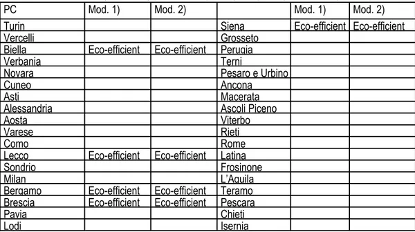
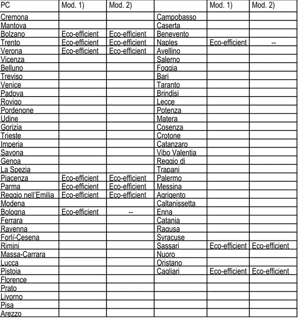
In Tables B.1 and B.2 we provide some detail for the eco-efficiency results of all the provincial capitals (PC’s), both for the Not-per capita and the Per-capita models.

By convention, we put eco-efficiency to 100 for the year 2000 for all PC’s. Then, we label as eco-efficient each municipality that shows in 2008 a score respectively above the value 101 for the Not-per capita model and the value 104 for the Per capita model. In Table B.1 provincial capitals are ordered according to the ISTAT conventional order (roughly from North-West to South-East), while in Table B.2 they are in alphabetical order.

More in detail, the eco-efficiency scores are obtained as follows. Recall that the scores for each capital must be calculated as deviations from L'Aquila’s ones. This also means that the year dummies represent the evolution through time of L'Aquila’s efficiency. In order to obtain the eco-efficiency of a given provincial capital in an year t, we then add to the value of the dummy for year t, the value of the relevant provincial time trend multiplied by the years past 2000 (2 in 2001, 3 in 2002, up to 9 in 2008).

Table B.1: Eco-efficiency results by provincial capital: 1) Not-per capita model; 2) Per capita model.

PC Mod. 1) Mod. 2) Mod. 1) Mod. 2)

Turin Siena Eco-efficient Eco-efficient

Vercelli Grosseto

Biella Eco-efficient Eco-efficient Perugia

Verbania Terni

Novara Pesaro e Urbino

Cuneo Ancona

Asti Macerata

Alessandria Ascoli Piceno

Aosta Viterbo

Varese Rieti

Como Rome

Lecco Eco-efficient Eco-efficient Latina

Sondrio Frosinone

Milan L’Aquila

Bergamo Eco-efficient Eco-efficient Teramo Brescia Eco-efficient Eco-efficient Pescara

PC Mod. 1) Mod. 2) Mod. 1) Mod. 2)

Cremona Campobasso

Mantova Caserta

Bolzano Eco-efficient Eco-efficient Benevento

Trento Eco-efficient Eco-efficient Naples Eco-efficient --Verona Eco-efficient Eco-efficient Avellino

Vicenza Salerno Belluno Foggia Treviso Bari Venice Taranto Padova Brindisi Rovigo Lecce Pordenone Potenza Udine Matera Gorizia Cosenza Trieste Crotone Imperia Catanzaro

Savona Vibo Valentia

Genoa Reggio di

La Spezia Trapani

Piacenza Eco-efficient Eco-efficient Palermo Parma Eco-efficient Eco-efficient Messina Reggio nell’Emilia Eco-efficient Eco-efficient Agrigento

Modena Caltanissetta

Bologna Eco-efficient -- Enna

Ferrara Catania

Ravenna Ragusa

Forlì-Cesena Syracuse

Rimini Sassari Eco-efficient Eco-efficient

Massa-Carrara Nuoro

Lucca Oristano

Pistoia Cagliari Eco-efficient Eco-efficient

Florence Prato Livorno Pisa Arezzo

Table B.2: Eco-efficiency results in detail: 1) Not-per capita model; 2) Per capita model.

PC Mod. Mod. 2 PC Mod. Mod. PC Mod. 1 Mod. 2 PC Mo Mod. 2

Agrigento 99,06 99,51 91,79 96,03 99,07 100,43 109 113,95 97,04 99 89,38 94 97,39 98,86 113 118,3 93,79 95,38 Ascoli 97,35 96,93 Beneven 96,37 96,05 109 113,95 92,88 95,55 94,54 94,16 93,12 92,88 113 118,3 93,34 96,56 90,58 90,5 88,77 88,86 119 125,71 93,95 97,51 88,93 89,47 86,71 87,45 120 127,27 96,52 100,8 88,6 89,24 85,96 86,82 Brescia 101 101,31 94,58 99,27 88,4 88,94 85,33 86,14 100 100,61 Alessandria 99,59 100,47 90,03 90,75 86,47 87,49 98, 98,86

PC Mod. Mod. 2 PC Mod. Mod. PC Mod. 1 Mod. 2 PC Mo Mod. 2 94,8 97,23 Asti 99,82 99,67 Bergam 100,63 100,93 100 101,9 94,13 97,87 98,16 98,18 99,36 100,05 102 103,83 94,85 99,38 95,24 95,69 96,79 98,12 106 108,3 95,73 100,84 94,68 95,94 96,61 99 105 107,62 98,61 104,75 95,52 97,03 97,86 100,76 Brindisi 97, 96,41 96,88 103,66 96,51 98,07 99,27 102,47 94, 93,4 Ancona 98,09 97,53 99,52 101,47 102,79 106,69 90, 89,53 95,62 95,03 97,9 100,01 101,52 105,82 89, 88,28 91,96 91,61 Avellino 96,87 97,12 Biella 102,02 101,5 88, 87,81 90,62 90,86 93,84 94,44 101,43 100,9 88, 87,28 90,63 90,9 89,69 90,86 99,49 99,24 90, 88,81 90,77 90,88 87,83 89,92 99,99 100,41 87, 86,09 92,79 93,01 87,29 89,77 101,98 102,48 Cagliari 101 100,03 90,48 90,68 86,88 89,56 104,17 104,52 100 98,72 Aosta 97,67 97,4 88,26 91,47 108,61 109,13 98, 96,38 95,01 94,84 85,52 89 108 108,55 98, 96,81 91,18 91,37 Bari 98,93 98,65 Bologna 100,62 100,07 100 98,09 89,66 90,56 96,86 96,68 99,35 98,78 102 99,31 89,48 90,54 93,55 93,74 96,78 96,46 106 102,94 89,43 90,46 92,59 93,51 96,59 96,91 105 101,64 91,22 92,52 92,99 94,09 97,84 98,21 Caltanisset 97, 96,68 88,76 90,14 93,53 94,61 99,25 99,46 94, 93,8 Arezzo 97,82 98,31 96,03 97,38 102,77 103,11 91, 90,03 95,23 96,18 94,04 95,49 101,49 101,83 89, 88,9 91,46 93,09 Belluno 99,7 99,42 Bolzano 104,57 105,16 89, 88,56 90,01 92,69 97,99 97,81 105,25 106,4 89, 88,15 89,89 93,11 95,02 95,2 104,52 106,51 91, 89,82 89,91 93,46 94,41 95,33 106,35 109,69 88, 87,19 Campobasso 97,26 96,79 Como 98,63 98,98 95,13 97,14 85, 89,76 94,42 93,95 96,42 97,17 Enna 95,6 94,65 Frosinone 97, 97,17 90,43 90,23 92,99 94,37 92,01 90,85 95, 94,5 88,74 89,15 91,9 94,29 87,36 86,28 91, 90,94 88,37 88,85 92,16 95,03 84,99 84,3 90, 90,02 88,14 88,49 92,56 95,72 83,92 83,08 89, 89,9 89,72 90,22 94,89 98,69 82,98 81,82 89, 89,71 87,12 87,62 92,78 96,93 83,74 82,49 91, 91,64 Caserta 98,29 98,65 Cosenza 80,62 79,23 89, 89,18 95,92 96,68 Ferrara 98,69 98,54 Genoa 100 99,38 92,35 93,74 96,5 96,52 98, 97,75 91,1 93,5 93,09 93,53 95, 95,13 91,2 94,08 92,02 93,24 95, 95,24

PC Mod. Mod. 2 PC Mod. Mod. PC Mod. 1 Mod. 2 PC Mo Mod. 2 93,57 97,36 92,73 94,23 97, 97,07 91,34 95,47 95,08 96,94 101 100,29 Catania 99,57 97,74 Cremon 99,54 99,19 93 95,01 99, 98,7 97,8 95,34 97,75 97,47 Florence 98,32 98,19 Gorizia 100 99,45 94,76 92,01 94,7 94,77 95,96 96 98, 97,86 94,09 91,35 94,02 94,78 92,39 92,86 95, 95,27 94,8 91,49 94,72 95,63 91,16 92,41 95, 95,41 95,67 91,56 95,56 96,42 91,27 92,76 96, 96,39 98,54 93,81 98,41 99,51 91,52 93,06 97, 97,32 96,81 91,56 96,67 97,85 93,67 95,56 100 100,58 Catanzaro Crotone 91,44 93,48 99, 99,02 Foggia Grosseto 97, 98,89 95, 97,03 91, 94,2 90, 94,07 90, 94,77 90, 95,41 92, 98,32 Chieti Cuneo 99,18 99,03 89, 96,53 97,23 97,24 Forlì 96,93 97,31 Imperia 99, 98,97 94,03 94,46 93,94 94,71 97, 97,15 93,18 94,4 89,81 91,2 93, 94,34 93,7 95,17 87,98 90,35 93, 94,25 94,37 95,88 87,47 90,29 93, 94,99 97,01 98,88 87,09 90,16 94, 95,67 94,86 96,86 91,58 98,96 96,79 99,46 95, 103,22

Isernia 97,52 97,06 Lecco 100,62 100,49 Mantova 98,3 97,82 Modena 96, 96,47 94,79 94,34 99,35 99,4 95,94 95,46 93, 93,48 90,9 90,73 96,78 97,27 92,37 92,16 88, 89,63 89,32 89,77 96,6 97,93 91,13 91,54 86, 88,41 89,06 89,59 97,85 99,45 91,23 91,72 86, 87,97 88,94 89,35 99,26 100,92 91,48 91,83 85, 87,46 90,66 91,22 102,78 104,85 93,62 94,12 86, 89,02 88,14 88,72 101,5 103,76 91,39 91,9 83, 86,32

L’Aquila 97,28 97,4 Livorno 98,55 98,31 Massa 97,16 97,11 Naples 101 99,15 94,45 94,85 96,3 96,18 94,26 94,43 100 97,42 90,46 91,38 92,84 93,09 90,23 90,84 98, 94,69 88,78 90,57 91,7 92,69 88,49 89,9 98, 94,69 88,42 90,55 91,93 93,1 88,08 89,75 99, 95,52 88,2 90,47 92,29 93,45 87,8 89,54 101 96,29 89,8 92,53 94,57 96,02 89,33 91,44 105 99,37

PC Mod. Mod. 2 PC Mod. Mod. PC Mod. 1 Mod. 2 PC Mo Mod. 2

La Spezia 98,63 98,48 Lodi 98,59 98,7 Matera 97,6 97,33 Novara 99, 99,04

96,42 96,43 96,36 96,76 94,91 94,74 97, 97,26 92,98 93,42 92,92 93,84 91,06 91,24 94, 94,49 91,89 93,1 91,8 93,63 89,51 90,4 93, 94,43 92,15 93,59 92,05 94,23 89,3 90,35 94, 95,21 92,55 94,03 92,43 94,77 89,22 90,23 95, 95,92 94,87 96,7 94,73 97,58 90,98 92,25 97, 98,93 92,76 94,74 92,61 95,71 88,49 89,85 96, 97,2

Latina 95,61 96,16 Lucca 97,59 97,37 Messina 98,29 96,96 Nuoro 92,02 93,04 94,9 94,8 95,92 94,2 87,38 89,07 91,04 91,31 92,35 90,55 85,01 87,71 89,49 90,49 91,1 89,55 83,94 87,13 89,27 90,45 91,2 89,32 83 86,5 89,19 90,36 91,44 89,04 83,78 87,9 90,95 92,4 93,58 90,86 80,65 85,1 88,46 90,01 91,35 88,33

Lecce 98,35 99,44 Macerat 99,57 99,55 Milan 99,26 100,38 Oristano 96,01 97,84 97,79 98,01 97,34 99,23 92,46 95,25 94,76 95,46 94,17 97,05 91,24 95,38 94,08 95,65 93,36 97,64 91,36 96,36 94,79 96,68 93,92 99,1 91,63 97,27 95,66 97,66 94,62 100,51 93,8 100,52 98,52 100,98 97,31 104,36 95,45 103,22 88,67 96,56 88, 91,23

Modena 96,43 96,47 Padova 99,08 99,07 Pesaro 98,92 98,47 Pordenone 100 99,99 93,21 93,48 97,07 97,3 96,84 96,42 98, 98,65 88,89 89,63 93,83 94,54 93,53 93,4 95, 96,3 86,86 88,41 92,93 94,5 92,56 93,08 95, 96,7 86,13 87,97 93,4 95,29 92,96 93,57 96, 97,96 85,53 87,46 94,02 96,02 93,5 94 97, 99,16 86,7 89,02 96,6 99,04 95,99 96,67 101 102,76 83,82 86,32 94,66 97,32 93,99 94,7 99, 101,44

Naples 101,34 99,15 Palermo 100,18 98,1 Pescara 98,34 98,51 Potenza 96, 95,9 100,41 97,42 98,69 95,87 95,99 96,48 93, 92,66 98,16 94,69 95,92 92,7 92,44 93,48 89, 88,58 98,32 94,69 95,53 92,21 91,21 93,18 87, 87,11 99,94 95,52 96,55 92,52 91,33 93,69 86, 86,42 101,74 96,29 97,73 92,77 91,59 94,14 86, 85,67 105,72 99,37 100,96 95,22 93,75 96,83 87, 86,94 104,78 97,68 99,49 93,11 91,54 94,88 84, 84,05

PC Mod. Mod. 2 PC Mod. Mod. PC Mod. 1 Mod. 2 PC Mo Mod. 2 94,43 94,49 93,9 97,34 96,19 97,43 92, 94,48 93,68 94,43 93,01 98,01 95,86 98,12 90, 94,42 94,31 95,21 93,5 99,55 96,95 99,68 91 95,2 95,09 95,92 94,14 101,05 98,2 101,2 91, 95,91 97,85 98,93 96,74 104,99 101,52 105,18 93, 98,91 96,05 97,2 94,82 103,93 100,11 104,13 91, 97,18

Nuoro Pavia 99,33 98,62 Pisa 96,28 95,11 Ragusa

97,44 96,64 92,98 91,52 94,3 93,69 88,6 87,13 93,51 93,43 86,5 85,33 94,11 94 85,7 84,3 94,85 94,5 85,04 83,23 97,57 97,26 86,13 84,12 95,74 95,35 83,21 80,99

Oristano Perugia 97,65 98,9 Pistoia 97,48 97,66 Ravenna 97, 99,36

94,98 97,04 94,74 95,22 94, 97,72 91,14 94,21 90,84 91,86 90, 95,09 89,61 94,09 89,24 91,16 88, 95,19 89,41 94,79 88,97 91,27 88, 96,12 89,35 95,44 88,84 91,3 88, 96,99 91,14 98,36 90,54 93,51 89, 100,19 87,1 98,6 84,81 95,48 105,18 109,61 95, 99,67

Reggio Rovigo 98,25 97,9 Syracus 98,9 98,35 Turin 98, 99,02

95,86 95,58 96,81 96,24 95, 97,21 92,27 92,32 93,5 93,17 92, 94,43 91 91,74 92,52 92,79 90, 94,37 91,08 91,96 92,91 93,23 90, 95,13 91,3 92,11 93,44 93,6 90, 95,83 93,41 94,45 95,92 96,2 93, 98,82 91,16 92,26 93,92 94,18 90, 97,07

Reggio 98,23 100,66 Salerno 98,59 98 Sondrio Trapani

95,82 99,64 96,36 95,73 92,22 97,59 92,91 92,51 90,95 98,32 91,79 91,97 91,02 99,93 92,04 92,24 91,23 101,5 92,42 92,44 93,33 105,53 94,72 94,83 91,07 104,52 92,6 92,68

Rieti 98,06 98,14 Sassari 99,29 100,42 Taranto 98,46 96,76 Trento 103 103,88 95,59 95,92 97,38 99,3 96,16 93,91 103 104,46 91,92 92,77 94,22 97,14 92,66 90,18 101 103,93

PC Mod. Mod. 2 PC Mod. Mod. PC Mod. 1 Mod. 2 PC Mo Mod. 2

90,57 92,62 93,99 99,24 91,66 88,77 105 109,83 90,7 92,89 94,72 100,68 91,98 88,4 108 113,32 92,71 95,36 97,42 104,56 94,21 90,11 113 119,69 90,39 93,26 95,57 103,44 92,04 87,51 113 120,43

Rimini 96,79 97,63 Savona 99,37 99,14 Teramo 97,64 97,66 Treviso 98, 98,46 93,73 95,18 97,51 97,4 94,97 95,22 96, 96,4 89,54 91,8 94,39 94,67 91,13 91,86 93, 93,38 87,65 91,09 93,63 94,66 89,6 91,16 92, 93,05 87,08 91,18 94,25 95,49 89,4 91,26 92, 93,54 86,63 91,21 95,01 96,25 89,34 91,3 92, 93,96 87,98 93,39 97,77 99,32 91,12 93,5 95, 96,62 85,21 91,1 95,96 97,63 88,65 91,22 93, 94,65

Rome 96,69 98,65 Siena 101,42 101,72 Terni 99,32 99,6 Trieste 98, 97,24 93,58 96,68 100,54 101,23 97,43 98,08 96, 94,61 89,35 93,74 98,32 99,67 94,3 95,55 93, 91,08 87,42 93,51 98,53 100,95 93,51 95,76 92, 90,2 86,8 94,09 100,19 103,15 94,1 96,82 92, 90,11 86,31 94,6 102,04 105,32 94,84 97,82 92, 89,95 87,6 97,38 106,08 110,08 97,57 101,17 95, 91,92 93,05 89,49 94,6 94,1 Udine 98,91 99,06 97,28 96,78 96,82 97,28 95,42 94,83 93,51 94,51 Verona 100,11 100,46 92,54 94,47 98,59 99,36 92,93 95,25 95,79 97,22 93,47 95,97 95,37 97,86 95,95 98,99 96,35 99,36 93,95 97,26 97,49 100,82 Varese 100,65 100,32 100,69 104,73 99,39 99,15 99,19 103,63 96,83 96,95 Vibo 97,24 96,55 96,66 97,52 94,38 93,6 97,93 98,95 90,38 89,78 99,35 100,33 88,68 88,59 102,89 104,15 88,3 88,18 101,63 102,98 88,06 87,72 Venice 97,96 97,24 89,63 89,32 95,43 94,62 87,02 86,64 91,72 91,08 Vicenza 98,24 98,74 90,32 90,2 95,84 96,82 90,27 90,11 92,25 93,92

PC Mod. Mod. 2 PC Mod. Mod. PC Mod. 1 Mod. 2 PC Mo Mod. 2 92,3 91,93 91,05 94,35 89,94 89,5 91,27 94,91 Verbania 98,3 97,86 93,37 97,74 95,92 95,52 91,12 95,88 92,35 92,24 Viterbo 96,87 96,67 91,11 91,64 93,85 93,78 91,21 91,84 89,7 90 91,45 91,97 87,84 88,87 93,59 94,29 87,3 88,51 91,35 92,08 86,9 88,1 Vercelli 99,25 98,5 88,28 89,77 97,33 96,46 85,55 87,13 94,16 93,46 93,34 93,15 93,9 93,66 References

[1] Ball, V.E., Lovell, C.A.K., Nehring, R.F., Somwaru, A., 1994, Incorporating undesirable outputs into models of production: An application to US agriculture, Cahiers d’Economique et Sociologie Rurale, 31, 59-73.

[2] Cameron, A. C., Trivedi, P. K., 2005. Microeconometrics, Methods and Applications, Cambridge University Press, New York.

[3] Carillo, F., Maietta, O.W., 2014. The relationship between economic growth and environmental quality: the contributions of economic structure and agricultural policies, NEW MEDIT, 13(1): 15-21. [4] Cornwell, C., Schmidt, P., Sickles, R.C., 1990. Production frontiers with cross-sectional and time-series variation in efficiency levels, Journal of Econometrics, 46(1-2): 185-200.

[5] Destefanis, S., Ofrìa, F., 2009. Forme proprietarie ed efficienza produttiva nei servizi socio-assistenziali. Un’analisi non-parametrica, Economia Pubblica, 39(5-6): 75-97.

[6] Fare, R., Grosskopfs, S., Lovell, C.A.K., Pasurka, C., 1989. Multilateral productivity comparisons when some outputs are undesirable: A nonparametric approach, Review of Economics and Statistics, 7l, 90-98.