ANALISI DEI MODELLI VALIDI PER LO STUDIO DEI
PROCESSI DI DEPOSIZIONE SECCA E SUI DATI METEO
PREVISIONALI DELL’ECMWF
(ANALYSIS OF MODELS FOR THE STUDY OF DRY
DEPOSITION PROCESSES AND ECMWF FORECAST
WEATHER DATA)
Indice
Indice 2
Abstract 4
1. Analysis of models to study dry deposition processes of pollutants in atmosphere onto urban surface. 5
1.1. Particle dry deposition velocity onto rough surfaces 5
1.2. Dry deposition process 6
1.3. Impaction processes and parameterization in the particle dry deposition 7
1.4. Short review of dry deposition models for gas and particle 7
1.5. A modified approach for dry deposition as inferred from various parameterization schemes 11
1.6. Comparison with experimental data 16
1.7. Conclusion – first activity 17
2. Preliminary study of compatibility between ECMWF forecast data and CALMET model. 21
2.1. Introduction – second activity 21
2.2. Technical notes of interest on the forecast model of ECMWF 21
2.3. Technical notes of interest on the CALMET model 23
2.4. Preliminary evaluation on the compatibility of the ECMWF data with the CALMET model 27
2.5. Conclusions – second activity 29
References – first activity 31
References – second activity 35
Abstract
The DEIM's research group in collaboration with ENEA – C.R. Bologna, has performed the following activities:
1. Analysis of models to study dry deposition processes of pollutants in atmosphere onto urban surface.
2. Preliminary study of compatibility between ECMWF forecast data and CALMET model.
Regarding the first activity, a dry deposition model, based on electrical analogy, is developed to analyze complex phenomena, such as inertial impact processes and wind turbulence effects, that influence the transport of pollutants in the interface between urban canopy and quasi-laminar sublayer.
The model allows the deposition rate assessment for particles with different diameters and various atmospheric conditions. A validation activity is performed by using some experimental data reported in literature for several Italian cities.
With regard the second activity, the work is aimed to verify the compatibility of ECMWF forecast data with CALMET.
This is a necessary step to build the CALMET data set input. Some empirical correlations as reported in literature as been identified to this purpose.
It is to be noted that the ECMWF does not provide land use data and average cells height, required for CALMET modeling. Such data can be obtained through some pre-processors included in the CALMET software package.
1.
Analysis of models to study dry deposition processes of pollutants in
atmosphere onto urban surface.
1.1.
Particle dry deposition velocity onto rough surfaces
Interest in atmospheric deposition has increased over the past decade due to concern about the effects of the deposition material entering the environment and subsequent health effects. Because of urbanization and industrialization, the formation of pollutants is quite inevitable and pollutants would be deposited on trees, grasses, crops, water bodies, and buildings with ecological and non-ecological impacts. There have been several studies to assess the deposition of atmospheric pollutants upon buildings (Dloske, 1995) or natural water that causes to water quality degradation and may harm aquatic ecosystems (Zufall et al., 1998).
In the nuclear field, if event of a severe accident and the release of radionuclides in the atmosphere occurs, certain key challenges arise, such as characterizing the specific types of release as well as studying the dispersion and deposition phenomena useful for defining effective mitigation measures and actions to protect the population.
Dry deposition process is recognized an important pathway among the various removal processes of radioactive pollutants in atmosphere. There isn’t a single accepted theoretical description of the involved dry deposition phenomena because of the complexity of the fluid-dynamic processes that influence the deposition flux, as well to lack of a complete experimental set of data covering all scenarios of interest.
Various experimental campaigns, performed in different international laboratories, allowed evaluations of deposition velocities for different types of pollutants and deposition surfaces. Nevertheless, there is a difficulty of generalization since the velocity values differ by four orders of magnitude for gases and three orders for particles (Sehmel, 1980; Pryor et al., 2007; Guha, 2008; Petroff et al., 2008). These issues limit the possibility to study the dry deposition process with a single modelling approach.
In this field research activities were focused to identify, among the models reported in literature, those approaches capable of representing dry deposition phenomena for several categories of pollutants and deposition surfaces (De Rosa et al., 1996; Ambrosio et al., 2015; Cervone et al. 2016). On the basis of this study, a new schema for parameterization of particle dry deposition velocity onto rough surfaces such as urban condition is proposed. The main aim is to develop
an approach to be easy to implement within atmospheric dispersion modeling codes as well as capable of dealing efficiently with different deposition surfaces.
The work involved comparisons with some experimental data reported in literature for different particle deposition scenario. The results shows that the proposed approach allows to catch, with good agreement, some aspects of phenomena involved in dry deposition processes for the examined environmental conditions and deposition surfaces.
1.2.
Dry deposition process
Dry deposition process refers to all phenomena of meteorological, chemical and biological nature that can influence a pollutant flux interacting with a ground surface, without involving the water into the atmosphere. The process is very complex and involves both gaseous pollutants and particulate of various granulometry and density, even if general phenomenological factors involving the two pollutant categories can be very different. The knowledge on particle dry deposition is far from being completely understood due to the complex dependences of deposition on particle size, density, terrain, vegetation, meteorological conditions and chemical species.
The main phenomena, that are considered to influence the deposition process, are described as follows:
transport due to atmospheric turbulence in the lower layer of the Planetary Boundary Layer (PBL), very near to the ground, called Surface Layer (SL). This process is independent of the physical and chemical nature of the pollutant and it depends only on the turbulence level; diffusion in the thin layer of air which overlooks the air-ground interface (named quasi-laminar sublayer resistance), where the dominant component becomes molecular diffusion for gasses, Brownian motion for particles and gravity for heavier particles;
transfer to the ground that exhibits a pronounced dependence on surface type with which the pollutant interacts (i.e. urban context, grass, forest, etc.).
Furthermore, the efficiencies of capture for the particles is connected to captation processes, which depend on both the surface typology of the deposits and obstacle dimensions.
In the case of gas, containment of a pollutant by a surface depends on the surface chemical property, which absorbs, dissolves or involves pollutant in chemical reactions; in case of particles the efficiency of pollutant capture is connected to resuspension and redeposition phenomena that depend both on the surface type and wind velocity. Moreover, the deposition
process changes quite a lot over the year, for example due to the seasonal variation of vegetation (with or without leaf) or over the day in connection with meteorological conditions (e.g. influence of temperature on leaf stoma).
1.3.
Impaction processes and parameterization in the particle dry
deposition
Brownian diffusion and eddy turbulence effects are a major contribution to the total dry deposition velocity for particles in the size range from 0.01 m to approximately a few micrometers. It is assumed to dominate the diffusion processes in the quasi-laminar sublayer surface. For particles of intermediate diameter dp (in the range about of 0.1 to 1 m), the process
strongly depends on atmospheric conditions, surface characteristics, and particle size.
Above this range, the deposition is dominated by other phenomena as inertial impaction characterized by the following interaction mechanisms (Petroff et al., 2008):
Inertial impaction. If the particle inertia is too large, the particle, transported by the flow towards an obstacle, cannot follow the flow deviation (particles may not be able to follow it as a result of inertia) and, consequently, can collide with the obstacle and remains on surface.
Turbulent impaction. In this mechanism, the particle has a sufficiently high velocity that turbulent eddies can give a transverse “free fight velocity”. So particles possess sufficient momentum to reach the surface (Epstein, 1997; Almohammed and Breuer, 2016; Kor and Kharrat, 2016).
The collection velocity for Brownian diffusion is classically related to Schmidt number 𝑆𝑐 = 𝜈𝑎/𝐷, being 𝜈𝑎 the cinematic viscosity of air and D Brownian diffusivity (Bott, 1995).
The efficiency of collection by impaction is classically related to the Stokes number 𝑆𝑡 = 𝑣𝑠𝑢∗2/𝑔 𝜈𝑎, where 𝑣𝑠 is the settling velocity, 𝑢∗ the friction velocity that represents the intensity
of atmospheric turbulence, and 𝑔 the gravity acceleration.
The parametrizations of deposition velocity, based on Schmidt and Stokes numbers, differ greatly between the models reported in literature, as described in the following sections.
A key concept to study the dry deposition process is the deposition velocity vd [m/s] (i.e. the
deposition velocity at a given height z) that links the pollutant vertical flux to the concentration measured at quota z [m] to the ground reference level:
vd = Fd
C(z) (1)
with Fd [g/(m2s)] pollutant flux removed per unit area and C(z) [g/m3] the pollutant
concentration at quota z.
Considering that the reciprocal of vd is the overall resistance to mass transfer, the influence of
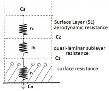
the various phenomena on deposition velocity can be expressed in terms of an electric analogy. On the basis of analogy with electrical circuits, the resistance to the mass transfer is configured as resistances in parallel and series circuits to describe transfer factor between air and surface. For gaseous pollutant collection, as shown in Fig. 1, it is possible to write the following relationship: |Fd| =C3− C2 ra = C2− C1 rb = C1− C0 rs (2)
where ra is the aerodynamic resistance which takes into account turbulence phenomenon in SL;
rb is the quasi-laminar sublayer resistance related to diffusion phenomenon for gas and
collisions due to Brownian motion for particles and rs is the surface resistance which depends
on nature of the receptor ground.
Based on the previous equation, the following relationship can be derived:
C3 = (ra+ rb+ rs)|Fd| (3)
Accordingly, the overall resistance formulation for gas can be given as follows:
vd = 1
Different studies are reported in literature (Wesely et al., 1985; Giorgi, 1986; Erisman et al., 1994; Padro et al., 1991; Padro, 1996; Wesely et al., 2001; Zhang et al., 2003; Kor and Kharrat, 2016) to evaluate parameters ra and rb.
The calculation of the gas surface resistance rs depends on the primary pathways for uptake,
such as diffusion through the leaf stomata and uptake through the leaf cuticular membrane. A revised parameterization, which includes a realistic treatment of the cuticle and ground resistance in winter (low temperature and snow-covered surfaces) as well the handling of seasonally-dependent input parameters, has been reported in (Zhang et al., 2003).
For particles pollutant, in SL region the turbulence acts on particles motion exactly like on gas, however the process is influenced also from gravity. Into the quasi-laminar sublayer, as above said, the deposition process is influenced especially from Brownian motion and gravity for heavier particles.
Figure 1. Electrical analogy for the dry deposition of gaseous pollutants
The resistance ra, rb and rs are considered in parallel to a second pathway-gravitational settling
defined as the reciprocal of settling velocity(Slinn and Slinn, 1980; Hicks et al., 1985; Hicks et al., 1987; Hanna et al., 1991; Seinfeld and Pandis, 1998).
Seinfeld and Pandis (1998) derived a dry deposition flux relationship based on the assumption that rs=0, and by equating the vertical fluxes in two layers over a surface to the total resistance
|Fd| =
C3 − C2
ra + vsc2 =
C2−C1
rb + vsc1 (5)
The velocity vd can be obtained by resolving the above equation as reported below:
vd = vs+
1
ra+ rb+ rarbvs (6)
where the product ra rb vs represents a virtual resistance.
The settling velocity vs grows in proportion to the square of particle diameter, dp, according to
the law of Stokes valid for particles with a diameter of up to 50 m:
vs =
dp2g(ρ
p− ρ𝑎)Cc
18𝑎
(7)
where p is particle density, a air density, aair kinematic viscosity and Cc is the Cunningham
factor (Seinfeld and Pandis, 1998):
cc = 1 +
a
dp(2,514 + 0,8 e
−0,55dp
a ) (8)
with a the mean free path of air.
As highlighted by Venkatram and Pleim (1999), the above expressions for dry deposition velocity of particles based on the electrical analogy are not consistent with the mass conservation equation.
Vertical transport of particles can be modeled by assuming that turbulent transport and particle settling can be added together as follows (Csanady, 1973):
𝑘𝑑𝐶
𝑑𝑧 + 𝑣𝑠C = F (9)
By integrating the above equation, it is possible to obtain the expression of the deposition velocity as follows:
𝑣𝑑 = 𝑣𝑠
[1 − 𝑒−𝑟(𝑧)𝑣𝑠] (10)
where vs is considered to be height invariant and r(z) is the total resistance to transport that can
be computed as a function of dp.
Note that, there might be little difference between the magnitudes of the dry deposition velocities estimated with Eq.s (6) and (10).
1.5.
A modified approach for dry deposition as inferred from various
parameterization schemes
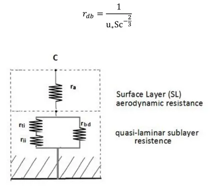
A new approach, based on the electrical analogy, is propose, to evaluate the resistance r in Eq. (10) for urban rough surfaces, as shown in Fig. 2.
It is to be noted that in urban-scale dispersion models, the lowest portion of the boundary layer is often represented using surface layer similarity parameterizations as described below. Boundary layer formulations of this type are only applicable in the inertial sublayer well above the building tops, but not in the immediate vicinity of the urban canopy elements where the flow locally depends on the particular building arrangement and thus has a rather complex structure.
As above said, interception and inertial forces may transport large particles across the viscous sublayer. A particle with a diameter greater than the sublayer height moving with the mean motion of the air will be deposited by interception when it collides with an obstacle. This occurs when the particle is traveling on an air streamline that passes within one particle radius of the obstacle. Inertial forces may lead to impaction and turbulent inertial deposition. Impaction occurs when the particle leaves the streamline since it cannot follow rapid changes in the air flow, and collides with an obstacle. Turbulent inertial deposition occurs when inertial energy derived from the component of air flow perpendicular to the surface (a turbulent eddy) carries a particle close to the surface (Zufall and Davidson, 1998).
Once a particle has traversed the viscous sublayer, it will interact with the surface. Depending on the characteristics of the contaminant and surface, a particle may stick or bounce off. There
may also be subsequent chemical reactions. Particle deposition by any combination of these transport mechanisms largely depends on atmospheric, surface, and particle characteristics (Zufall and Davidson, 1998).
The scheme of deposition processes upon the canopy of urban surfaces has been modified to include the particle rebound or resuspension phenomena together with Brownian diffusion, impaction process, and turbulent transfer.
In the proposed approach the aerodynamic resistance ra (i.e. contribution to the deposition due
to the atmospheric turbulence in the SL) is connected in series with the resistance rql across the
quasi-laminar sublayer to take into account mechanisms of diffusion by Brownian motion and impaction phenomena (Fig. 2). The resistance rql is evaluated by considering two resistances in
parallel, that is: the resistance rbd, which represents the Brownian diffusion, and the resistance
ri, which allows to treat impaction processes.
The resistance ri is evaluated by considering two resistances in series:
resistance rii that takes into account the inertial impact condition,
resistance rti that considers the effects resulting from turbulent impaction.
These last assumptions allow to take into consideration effects on particle concentration coming from both the inertial and turbulent impaction (i.e. reciprocal influence of the two impact processes on dry deposition efficiency).
Accordingly, the overall resistance r in eq. (10) can be evaluated by the using the following equations:
r = ra+ rql (11)
where rql is evaluated by using the following relationship:
1 rql = 1 rbd+ 1 ri (12)
and ri is obtained as follows:
Following the usual methods of micrometeorology for homogeneous terrain, the pollutant concentration flux can be expressed in terms of the local flux–gradient relationship (surface-layer similarity theory) (e.g. Businger 1973). Therefore the resistance ra can be determined by
using Monin–Obukhov similarity theory as follows (Hanna et al., 1991; Seinfeld and Pandis, 1998; Baldocchi et al., 1995; Voldner et al., 1986; Wesely and Hicks 1977; Maryon et al., 1996; Hicks, 1982; Slinn et al., 1978):
ra = 1 ku∗[ln
z
zo− Ψh] (14)
being z0 the surface roughness height above the displacement plane and k the von Karman
constant (generally equal to 0.4).
Brandt et al. (2002) suggested the following relationship for calculating parameter Ψh in Eq.
(15): Ψh = −5z L 𝑤𝑖𝑡ℎ 𝑧 𝐿> 0 (𝑠𝑡𝑎𝑏𝑙𝑒 𝑎𝑡𝑚𝑜𝑠𝑝ℎ𝑒𝑟𝑖𝑐 𝑐𝑜𝑛𝑑𝑖𝑡𝑖𝑜𝑛𝑠) (15) Ψh = e{0,598+0,390 ln(− z L)−0,09[ln(− z L)] 2 } 𝑤𝑖𝑡ℎ 𝑧 𝐿< 0 (𝑢𝑛𝑠𝑡𝑎𝑏𝑙𝑒 𝑎𝑡𝑚𝑜𝑠𝑝ℎ𝑒𝑟𝑖𝑐 𝑐𝑜𝑛𝑑𝑖𝑡𝑖𝑜𝑛𝑠)(16)
where L is the Monin-Obukhov length computed as follows:
L =u∗
3c pρT̅
kgH (17)
with cp specific heat at constant pressure, T̅ average temperature in SL, and H sensible heat.
For the resistance rbd various models predict a functional dependence on Sc number such that
in general:
rbd = 1
𝑢∗c Sc
p (18)
The parameter p usually lies between 1/2 and 2/3 with larger values for rougher surfaces. For example,
Slinn and Slinn (1980) suggested a value of 1/2 for water surfaces. Slinn (1982) suggest a value of 2/3 for vegetated surfaces. Zhang et al. (2001) used values of p varying with land use categories.
In this work it is assumed in Eq. (18) the following relationship:
𝑟𝑑𝑏 = 1 u∗Sc−23
(19)
Figure 2. New schematization based on electrical analogy for
parametrization of particles deposition velocity.
The transport of particles by Brownian diffusion represented as function of Sc2/3 in eq. (19) is
recommended in various works on the basis of theoretical and empirical results (Wesely and Hicks 1977; Paw, 1983, Hicks et al., 1987; Pryor et al., 2009; Kumar and Kumari, 2012). It is proposed to evaluate the resistance for inertial impact process rii in Eq. (13) by using the
following relationships valid for rough surfaces:
rii= 1 u∗( St 2 St2+ 1)R (20)
Various Author suggested this formula or similar for impaction efficiency as function of smooth surfaces and surfaces with roughness elements (Slinn, 1982; Giorgi, 1986; Peters and Eiden 1992).
Note that particle rebound is also included via the factor R (Giorgi, 1988; Zhang et al., 2001). Slinn (1982) suggested the following form for R:
R = 𝑒(−𝑏√𝑆𝑡) (21)
where b is an empirical constant, often assumed to be 1 (Giorgi, 1986; Zhang et al., 2001). In this work it is assumed b=2 as suggested in (Nemitz et al., 2002). For the calculation of resistance rti, general assumptions are reported below.
As well known, empirical relations of turbulent deposition are typically presented in terms of the dimensionless particle relaxation time +:
𝜏+ = 𝜏
𝑢∗2
(22)
where is the particle relaxation time defined, for a spherical particle, as follows:
𝜏 = 𝑑𝑝
2𝜌 𝑝𝐶𝑐
18𝜇 (23)
Various models predict a functional dependence of resistance turbulent impact phenomena rti
on + as follows:
rti =
1
𝑢∗m+𝑛𝑅 𝑎𝑙𝑙 𝑠𝑢𝑟𝑓𝑎𝑐𝑒𝑠 (24)
For turbulent deposition in pipe flows, the following regimes have been observed (Guha, 1997, 2008):
Regime with about +<0.1 (very small particles); Brownian diffusion becomes significant and
deposition is affected by a combination of Brownian and eddy diffusion. For the Brownian regime the deposition velocity is function of the Schmidt number;
Regime with about 0.1<+<30; particle motion is strongly dependent on turbulent fluctuation
in the fluid flow and the deposition velocity increases with +. For larger particles the deposition
velocity can be considered proportional to a second power of +.
Regime with about +>30; the particles have large inertia and the effect of turbulence on particle
motion is significantly reduced and the gravity effect is dominant.
For most trace gases, the uncertainty associated with the value of exponent n is not critical, but for very slowly diffusing quantities such as aerosol particles, the uncertainties become large. This remains a subject for research.
It is to be noted that in Eq. (24) there is the correction factor R related to the collection efficiency for rebound evaluated by Eq. (21). This allows to take into account the functional dependence of rebound phenomena on turbulent impact conditions.
The constants m and n in Eq. (24) have been evaluated by fitting some data reported in literature for urban surfaces. The result was for m and n the values of 0.05 and 0.75, respectively.
1.6.
Comparison with experimental data
The new approach for computing deposition velocity vd is validated by comparison with
experimental data reported in literature for several meteorological conditions and deposition urban surfaces.
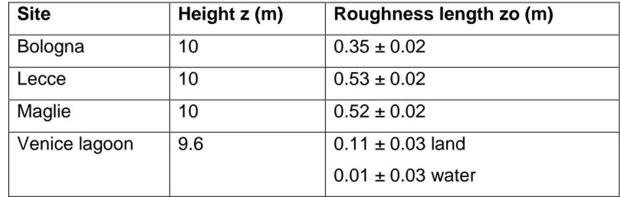
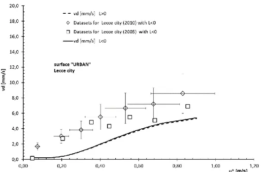
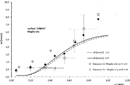
Figures 3 through 6 show experimental data for urban area in terms of deposition velocity as function of frictional velocity u* (Donateo and Contini, 2014). The datasets were taken in different experimental campaigns over a wide range of surface roughness conditions, from almost smooth surfaces (i.e., iced surfaces in Antarctica) to surfaces with different degrees of complexity: urban background, urban canopy, and industrial district (in Italy) or Venice lagoon surface (Italy). Summary of experimental sites in terms of measurement height (z), and roughness height zo are reported in Table 1.
In all figures the vertical bars present errors of 30%.
On the whole, a good agreement between the prediction trend obtained by using the proposed model and the examined experimental data is found.
In particular, it can be observed good predictions for u* values above about 0.3 m/s. Only limited effect of stability is observed with a slight reduction of the deposition velocities at fixed in stable conditions. This aspect is captured by the proposed approach.
Table 1. Summary of experimental sites and instruments used in aerosol sampling reported in (Donateo and Contini, 2014).
Site Height z (m) Roughness length zo (m)
Bologna 10 0.35 ± 0.02
Lecce 10 0.53 ± 0.02
Maglie 10 0.52 ± 0.02
Venice lagoon 9.6 0.11 ± 0.03 land
0.01 ± 0.03 water
1.7.
Conclusion – first activity
The ATMES (Atmospheric Transport Model Evaluation Study) report, relevant to study of models for the evaluation of radioactive pollutants disperse in the ambient atmosphere, highlighted that the highest uncertainties are in the parametrization of source terms and dry and wet deposition velocities (Klug et al. 1992).
In literature there are several models, but no one is able to treat exhaustively most of phenomenologies related to pollutants deposition because of many complex involved processes. A review of the existing mechanistic models emphasizes the wide variety of ways that captation can take place, however, a comparison of two similar scenarios provides large discrepancies each other, which can reach two orders of values for same particle diameter.
As highlighted by Sehmel (1980), the measurements of deposition velocity carried out by different international laboratories don’t allow to draw general conclusions due to experimental uncertainness.
The bibliographical study of experimental tests performed to evaluate dry deposition velocities for vegetative canopy (i.e. experiment in situ), or derived by wind tunnel measurements, demonstrates a substantial number of differences that are more pronounced for forest canopies or in the accumulation range.
For the same typology of pollutant, experimental data shows that, for gas, the values of deposition velocity differ even by four order of magnitude and, for particles, by up to three order of magnitude.
The main aim of our research activity was to develop an approach to be easy to implement within atmospheric dispersion modeling codes as well as an approach capable of dealing efficiently with different deposition surfaces for several radioactive pollutants. Some parametrizations reported in literature can be applied for multiple size classes (i.e. particle diameter), or they are based upon a number of assumption which may be frequently be violated in practice (Pryor et al., 2007), or even they are strongly dependent by a number of parameters combination as land use classification and seasonal categories.
After the study of the main phenomenologies involved in dry deposition processes (Ambrosio et al., 2015; Cervone et al., 2016) different models, which use several parametrizations for variables defining deposition process and for dimensionless factors employed for modelling, were examined.
On the basis this study, a new scheme for particles deposition velocity based on electrical analogy is propose, to evaluate the resistances for urban rough surfaces.
It is worth to note that the correlation obtained with the new schematization is based on the hypothesis that the impact phenomena in the quasi-laminar sublayer can be affected by specific local features of the mutual influence of inertial impact processes, and turbulent impact phenomena. The proposed approach is further modified to take in consideration the rebound phenomena.
The validation work, carried out by using some experimental data from literature, allowed to verify the goodness of the proposed approach.
Research works concerning further validation activities of deposition processes onto urban surfaces are in progress.
Figure 3. Deposition velocity predictions as functional dependence from friction velocity 𝑢∗ and comparison with measurement datasets relevant to Bologna city, as reported in (Donateo and Contini,
2014). The vertical bars present errors of 30%.
Figure 4. Deposition velocity predictions as functional dependence from friction velocity 𝑢∗ and comparison with measurement datasets relevant to Lecce city, as reported in (Donateo and Contini,
Figure 5. Deposition velocity predictions as functional dependence from friction velocity 𝑢∗ and comparison with measurement datasets relevant to Maglie city, as reported in (Donateo and Contini,
2014). The vertical bars present errors of 30%.
Figure 6. Deposition velocity predictions as functional dependence from friction velocity 𝑢∗ and comparison with measurement datasets relevant to Venice city, as reported in (Donateo and Contini,
2.
Preliminary study of compatibility between ECMWF forecast data and
CALMET model.
2.1.
Introduction – second activity
As of today, the study of pollutant dispersion in atmosphere, as the estimation of productivity of sites for the production of wind energy [1, 2], represents an example of application that require an accurate reconstruction of the three-dimensional wind filed or, more in general, of the meteorological fields that characterize the site.
Such studies, especially with complex orography, in order to produce highly accurate results must be conducted with a high resolution (~100m).
For this purpose, many authors have selected the diagnostic model CALMET as promising in order to determine the meteorological fields on the local scale starting from forecast data on the regional scale. Until today, the work have been carried on using forecast data that can be directly interfaced with the CALMET model, as the one produced by the meteorological MM5 or WRF [3-5].
Furthermore, in principle this approach can be used to analyze pollutant dispersion on forecast data.
The attraction to the possibility of working on this aspect and the availability of provisional data at high resolution produced by the European Centre Medium-Range Weather Forecast (ECMWF) lead to a verification of the formal compatibility of the provisional data with the input data required by CALMET as a first evaluation of compatibility. This approach would allow for an high resolution reconstruction of the meteorological data that are required to deploy forecast simulations of pollutant dispersion in atmosphere in almost real time, for a short range (72-90 hours).
2.2.
Technical notes of interest on the forecast model of ECMWF
ECMWF is an independent inter-govern organization founded in 1975 and today it is maintained by the European Union with some additional contributors. Its purpose is to provide medium-term (15 days) global weather forecast to member states, contributors and all parties that who have subscribed to their service. Furthermore, it promotes and carries on research in
the field of weather forecast and implements the MARS database, the biggest archive of weather data in the world as of today.
The ECMWF forecast system is built on many components: - general atmospheric circulation model;
- oceanic wave model; - Earth surface model;
- general oceanic circulation model;
- side models for data acquisition and previous forecast storage.
Figure 7. A sigma-p coordinate system representation [7].
The general atmospheric circulation model is coupled to the oceanic wave model to obtain a global model for Earth’s atmosphere. Its formulation is based on two different set of equations, a diagnostic one and a prognostic one. The first set describes the pressure, density, temperature
and height fields, while the second describes the horizontal components of the wind field, surface pressure, temperature and moisture content.
An additional set of equations determines hydrometric variations such as rain, snow, liquid water and ice inside clouds, etc.
The various models are coupled bi-directionally in order to take into account for the relative interactions. In this way the general model can account for energy (wind, heat, etc.) and mass (precipitation and evaporation) exchanges among the different environment components. About the three-dimensional representation of the fields, the model is based on a reduced Gaussian grid to represent surface quantities and a sigma-level or sigma-p system of coordinates for vertical quantities (Fig. 7). The Gaussian grid can take into account for the deformation generated by the convergence of the meridians: going from the tropics towards the poles, in order to maintain the distance between two points of the grid, their number is reduced.
From the horizontal point of view the forecast in lat/lon coordinates can reach a resolution of 0.125° (that corresponds to a distance along the meridians of about 13.5 km in the south direction); in the future it is expected to reach a resolution of ~9/5 km. On the vertical side, the model is subdivided in 137 levels. The sigma-p vertical system of coordinates has been developed in such a way to have an higher resolution on the lower troposphere, following the Shape of the Earth’s crust, while having a lower resolution towards the stratosphere, where the variations to be reproduced are smaller.
Forecasts are delivered from ECMWF two times a day, at 00:00 and 12:00 (Universal Coordinated Time – UTC). Forecast of the approaching 144 hours are available at 03:00 and 15:00, while the remaining forecasts (up to 240 hours) are available at 06:00 and 18:00. All the quantities, for the first 90 hours, are available with a temporal resolution of one hour.
The forecasts are released with different types of representations, i.e. with the 137 level atmospheric model, pressure level model, etc. Meteorological fields are available on the representation that is selected.
2.3.
Technical notes of interest on the CALMET model
The CALMET model is a diagnostic interpolator that builds three-dimensional fields of meteorological quantities. In order to produce its analysis it requires as input many files with meteorological and geophysics data along with a control variable file.
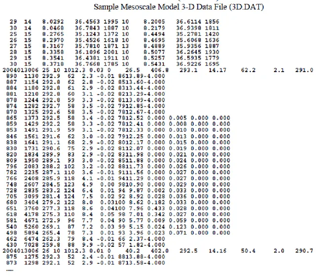
Figure 9. An example of the 3D.DAT file for a generic cell for CALMET
In particular, among the many options available in the control file we are interested in the IPROG variable, in group 5, that enables the use of prognostic data. This variable accepts 6 options: 3 of them (3, 4, 5) are reserved to the direct use of the output of MM4 and MM5 models, while the remaining 3 (13, 14, 15) can be selected to use the output form MM4, MM5, NAM (ETA), RUC or RAMS, WRF that must be reformatted with the proper preprocessor (CALMM5, CALAETA, CALRUC, CALRUMS). Since in general the output are formatted in ASCII format in a file with a well-defined structure (3D.DAT), it is possible to reformat the ECMWF data in the same manner.
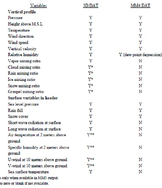
Figure 10. Weather data available in the 3D.DAT file and MM4.DAT file.
As we can see in Fig. 8, at the beginning of the file are reported the variables that describe the features of the forecast data, including the temporal range, the geographic domain and the parameters of the grid. The file continues (Fig. 9) with the repetition, as many times as the number of cells in the grid, of data blocks with meteorological data of the single cell. Among the surface quantities, we can find the surface pressure, rain amount e cloud coverage, while for the vertical levels we can find pressure, height, temperature, wind velocity and direction.
To the default variables at each level there can be some additional optional ones such as vertical wind velocity, relative humidity, vapor mixing ratio, cloud and rain mixing ratio, ice and snow mixing ratio and the groupel mixing ratio.
Figure 11. Horizontal and vertical geographic reference for the quantities in 3D.DAT [7]. The full list of the quantities inside the 3D.DAT file and the format of the different information blocks are available in the literature given with the CALMET code [7] (Figs. 10-11).
2.4.
Preliminary evaluation on the compatibility of the ECMWF data with
the CALMET model
Considering the fact that CALMET is able to work with prognostic data that are properly formatted, we evaluated the possibility of using the forecast data generated by ECMWF.
Among the various model that are available, we find of use the model that describes the surface weather quantities and the vertical one that is based on the sigma-p coordinate (137 levels, standard atmosphere ICAO-1976). The forecast up to 90 hours is of particular interest since it has a time step of 1 hour.
The ECMWF weather data are distributed in the GRIB format, that is not directly compatible with CALMET that required ASCII data as input. It is therefore necessary to use some tools (i.e. CDO) to convert the format and extract the weather data that is required for CALMET. On the majority of cases the weather data from ECMWF are compatible with the data required by CALMET, with some simple conversion of units of measures. However in some cases it is required to obtain some derivative quantities using empiric or semi-empiric correlations available in literature [8-10].
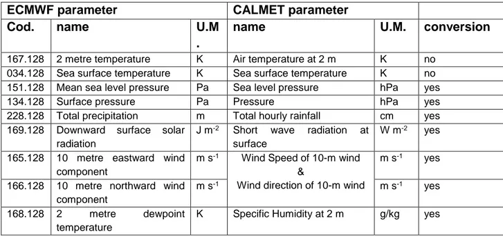
A synthesis of the useful ECMWF data and corresponding CALMET equivalents is available in Tab. 2 for the surface data and in Tab. 3 for the vertical data.
Table 2. weather surface data form ECMWF and corresponding CALMET variable.
ECMWF parameter CALMET parameter
Cod. name U.M
.
name U.M. conversion
167.128 2 metre temperature K Air temperature at 2 m K no
034.128 Sea surface temperature K Sea surface temperature K no
151.128 Mean sea level pressure Pa Sea level pressure hPa yes
134.128 Surface pressure Pa Pressure hPa yes
228.128 Total precipitation m Total hourly rainfall cm yes
169.128 Downward surface solar radiation
J m-2 Short wave radiation at
surface
W m-2 yes
165.128 10 metre eastward wind component
m s-1 Wind Speed of 10-m wind
&
Wind direction of 10-m wind
m s-1 yes
166.128 10 metre northward wind component
m s-1 m s-1 yes
168.128 2 metre dewpoint
temperature
K Specific Humidity at 2 m g/kg yes
From a comparison of the documentation of the CALMET model and the ECMWF forecast, the quantities 2 metre temperature and sea surface temperature can be used as-is, without any conversion. For the quantities mean sea level, surface pressure and total precipitation, they only require a change of scale. The conversion of the downward surface solar radiation is simple, since we need only to convert from deposited energy to incoming power, and similarly for the wind components, for which we need to convert from the eastward and northward components
to the wind direction and speed, as required by CALMET. Finally, the 2 metre dew point temperature is used to compute the specific humidity at 2 metre [8 - p. 38].
Table 3. Weather vertical data form ECMWF and corresponding CALMET variable.
ECMWF parameter CALMET parameter
Cod. name U.M. name U.M. conversion
130 Temperature K Temperature K no 131 Eastward wind component m s-1 Wind Speed & Wind direction m s-1 yes 132 Northward wind component m s-1 m s-1 yes
133 Specific Humidity kg kg-1 Relative Humidity % yes
135 Vertical velocity Pa s-1 Vertical velocity m s-1 yes
From the vertical model we can use the five quantities that are given in Tab. 2. As in the previous case, the temperature of the level does not require any conversion, and the conversion for the wind components is the same as the previous case. For the humidity, the ECMWF data set includes the specific humidity, while CALMET requires the relative humidity. The conversion between these two variables can be carried out through a semi-empirical correlation among the relative humidity, the specific humidity, the pressure and the saturation pressure of the level [8 – p. 38, 9 – p. 113-114]. Finally, the vertical velocity is given in Pa/s, so it must be converted in m/s in order to use it in CALMET [10 – p. 4-5].
Furthermore, standing that the ECMWF is a complete set of data, there is no data about land use and average cell height. These quantities are required to build the 3D.DAT file, but they can be generated from different CALMET preprocessors using different data sources (NOAA, Corine Land Cover, etc.), keeping in mind to guarantee the correct geolocalization.
2.5.
Conclusions – second activity
This activity has been focused on the verification of the availability of weather data required by the prognostic input in the CALMET model from the weather data available in the forecast data generated by the ECMWF.
It has been verified that a large section of the ECMWF data are compatible with the CALMET model, while others can be deduced using empirical and semi-empirical correlations.
Furthermore, it has been verified that, even in its completeness, the ECMWF model does not provide land use information and average cell heights, data that is required by CALMET. This
data can however be obtained from other preprocessors already available in the CALMET/CALPUFF software suite, that start from different sources such as NOAA, Corine Land Cover, etc.
References – first activity
1. Almohammed N., Breuer, M. 2016. Modeling and simulation of particle-wall adhesion of aerosol particles in particle-laden turbulent flows. International Journal of Multiphase Flow, 85, 142-156.
2. Ambrosio G., Buffa P., Caltabellotta G., Giardina M., Palermo G., Raniolo I., Ventura F., 2015. Definizione della metodologia e degli input necessari per l’esecuzione di analisi integrate CALMET-CALPUFF ai fini della valutazione della dispersione di inquinanti radioattivi in atmosfera, rapporto di ricerca ENEA n. ADPFISS-LP1-048, 2015. http://openarchive.enea.it/bitstream/handle/10840/6997/ADPFISS-LP1-048.pdf?sequence=1
3. Bott, T.R., 1995. Fouling of Heat Exchangers, Elsevier.
4. Brandt, J., Christensen J. H., Frohn L.M. 2002. Modelling transport and deposition of caesium and iodine from the Chernobyl accident using the DREAM model Atmos. Chem. Phys., 2, 397–417.
5. Businger J. A., 1973. Turbulent transfer in the atmospheric surface layer. Workshop on Micrometeorology, D. A. Haugen, Ed., Amer. Meteor. Soc., 67–100.
6. Cervone I., Lombardo C., Giardina M., Buffa P., Palermo G., 2016. Modelli per calcoli di concentrazione di materiale radioattivo disperso a breve-medio raggio in aree caratterizzate da configurazioni architettoniche tipiche delle principali città italiane, rapporto di ricerca ENEA n. ADPFISS-LP1-070 Rev. 0, 2016, http://openarchive.enea.it/handle/10840/8156.
7. Csanady G.T., 1973. Turbulent Diffusion in the Environment. Reidel, Dordrecht, Holland.
8. De Rosa F., Diamanti D., Mari R. 1996. RADCAL: a New Physically Based Module for the Prediction of Radioactive Chain Behaviour, rapporto di ricerca ENEA, Pubblicato su: Energia Nucleare, Anno 13, N. 3, 1996, http://hdl.handle.net/10840/2108, 1996.
9. Dloske DA. 1995. Deposition of atmospheric pollutants to monuments, statues and buildings. Sci Total Environ 167, 15–31.
10. Donateo A., Contini D. 2014. Correlation of Dry Deposition Velocity and Friction Velocity over Different Surfaces for PM2.5 and Particle Number Concentrations, Hindawi Publishing Corporation Advances in Meteorology Volume 2014, Article ID 760393, 12 pages http://dx.doi.org/10.1155/2014/760393
11. Epstein, N., 1997. Elements of particle deposition onto nonporous solid surfaces parallel to suspension flows. Exp. Therm. Fluid Sci., 14 (4),323–334.
12. Erisman, J. W., Van Pul, A., and Wyers, G. P., 1994. Parameterization of surface resistance for the quantification of atmospheric deposition of acidifying pollutants and ozone, Atmos. Environ., 28, 2595–2607.
13. Giorgi, F. 1988. Dry deposition velocities of atmospheric aerosols as inferred by applying a particle dry deposition parameterization to a general circulation model. Tellus, 40B:23–41.
14. Giorgi, F., 1986. A particle dry deposition parameterization scheme for use in tracer transport models. J. Geophjx Res., 91, 9794-9806.
15. Guha, A., 1997. A unified eulerian theory of turbulent deposition to smooth and rough surfaces. Journal of Aerosol Science, 28(8), 1517–1537.
16. Guha, A., 2008. Transport and deposition of particles in turbulent and laminar flow. Annual Review of Fluid Mechanics, 40, 311–341.
17. Hanna S.R., Gifford, F.A., Yamartino, R.J., 1991. Long Range Radioactive Plume Transport Simulation Model/Code – Phase I. USNRC Division of Contracts and Property Management, Contract Administration Branch, P-902, Washington, DC 20555. Technical report.
18. Hicks, B.B. 1982. Critical assessment document on acid deposition, ATDL Contributory file 81/24. Atmospheric turbulence and diffusion laboratory, NOAA, Oak Ridge, Tennessee.
19. Hicks, B.B., Baldocchi, D.D., Hosker ,R.P., Hutchison, B. A., Matt, D. R., McMillen, R.T., Satterfield L. C., 1985. On the Use of Monitores Air Concentrations to Infer Dry Deposition, NOAA Technical Memorandum ERLO ARLZ141.
20. Hicks, B.B., Baldocchi, D.D., Meyers, T.P.,Hosker, R.P., Jr., Matt, D.R. 1987. A preliminary multiple resistance routine for deriving dry deposition velocities from measured quantities. Water Air Soil Pollut, 36, 311–330.
21. Klug W., Graziani G., Grippa G., Pierce D., Tassone C. 1992. Evaluation of long range atmospheric transport models using environmental radioactivity data from the Chernobyl accident, The ATMES Report, Elsevier Applied Science, London and New York.
22. Kor, P., Kharrat, R., 2016. Modeling of asphaltene particle deposition from turbulent oil flow in tubing: Model validation and a parametric study. Petroleum, 2 (4), 393-398. 23. Kumar, R., Kumari, K. M. 2012. Experimental and Parameterization Method for Evaluation of Dry Deposition of S Compounds to Natural Surfaces, Atmospheric and Climate Sciences, 2, 492-500
24. Maryon R.H., Saltbones J., Ryall D.B., Bartnicki J., Jakobsen H.A., Berge E. 1996. An intercomparison of three long range dispersion models developed for the UK meteorological office, DNMI and EMEP. UK Met Office Turbulence and Diffusion Note 234. ISBN: 82-7144-026-08.
25. Nemitz E., Gallagher M. W., Duyzer J.H., Fowler D. 2002. Micrometeorological measurements of particle deposition velocities to moorland vegetation Q. J. R. Meteorol. Soc., 128, 2281–2300.
26. Padro J. 1996. Summary of ozone dry deposition velocity measurements and model estimates over vineyard, cotton, grass and deciduous forest in summer, Atmos. Environ., 30, 2363–2369.
27. Padro J., Hartog G., Neumann H. H. 1991. An investigation of the ADOM dry deposition module using summertime O3 measurements above a deciduous forest, Atmos. Environ., 25, 1689– 1704.
28. Paw U.K.T. 1983. The rebound of particles from natural surfaces. Journal of Colloid Interface Science 93, 442–452.
29. Peters K., Eiden R. 1992. Modelling the dry deposition velocity of aerosol particles to a spruce forest. Atmospheric Environment 26A, 2555-2564.
30. Petroff, A., Mailliat, A., Amielh, M., and Anselmet, F., 2008. Aerosol dry deposition on vegetative canopies. Part I: Review of present knowledge, Atmos. Environ., 42, 3625–3653.
31. Pryor S. C. , Barthelmie R. J., Spaulding A. M, Larsen S. E., Petroff A. 2009. Size-resolved fluxes of sub-100-nm particles over forests. Journal of Geophysical Research,114, D18212.
32. Pryor S.C., Gallagher M., Sievering H., Larsen S. E., Barthelmie R. J., Birsan F., Nemitz E., Rinne J., Kulmala M., Gro¨ Nholm T., Taipale R., Vesala T. 2007. Review of measurement and modelling results of particle atmosphere–surface exchange Volume 60, Issue 1, 42–75.
33. Sehmel G. A., 1980. Particle and gas dry deposition: a review. Atmos. Environ., 14, 983-1011.
34. Seinfeld J. H., Pandis S.N. 1998. Atmospheric chemistry and Physics – John Wiley&Sons, New York.
35. Slinn S.A., Slinn W.G.N. 1980. Predictions for particle deposition on natural waters. Atmos. Environ., 14, 1013-1016
36. Slinn W.G.N. 1982. Predictions for particle deposition to vegetative surfaces. Atmospheric Environment 16, 1785-1794.
37. Slinn W.G.N., Hasse L., Hicks B.B., Hogan A.W., Lal D., Liss P. S., Munnich K.O., Sehmel G.A., Vittorri O. 1978. Some aspects of the transfer of atmospheric trace constituents past the air-sea interface. Atmospheric Environment 12, 2055-2087. 38. Venkatram A., Pleim, J. 1999. The electrical analogy does not apply to modeling dry
deposition of particles, Atmos. Environ., 33, 3075–3076,.
39. Voldner E.C., Barrie L.A., Sirois A. 1986. A literature review of dry deposition of oxides of sulphur and nitrogen with emphasis on long-range transport modelling in North America. Atmos. Environ. 20. 2101-2123.
40. Wesely M.L., Hicks B.B. 1977. Some factors that affect the deposition rates of sulfur dioxide and similar gases to vegetation. J. Air Polka. Control Ass. 27, 1110-l 116. 41. Wesely, M. L., Cook, D. R., Hart, R. L., Speer, R. E., 1985. Measurements and
Parametrization of article Sulfur Deposition over Grass, Journal of Geophysical Research, 90, 2131-2143.
42. Wesely, M. L., Doskey, P. V., and Shannon, J. D., 2001. Deposition Parameterizations for the Industrial Source Complex (ISC3) Model, report to U.S. EPA, Argonne National Laboratory, USA.
43. Zhang L., Brook, J. R., Vet, R. 2003. A revised parameterization for gaseous dry deposition in air-quality models Atmos. Chem. Phys., 3, 2067–2082.
44. Zhang L., Gong S., Padro J., Barrie L. 2001. A size-segregated particle dry deposition scheme for an atmospheric aerosol model Atmospheric Environment, 35, 549-560 45. Zufall M. J., Davidson C. I. 1998. Dry Deposition of Particles from the Atmosphere,
Air Pollution in the Ural Mountains: Environmental, Health and Policy Aspects, Springer Netherlands, ISBN: 978-94-010-6192-6, pp 55-73.
46. Zufall M., Davidson C., Caffrey P., Ondov J. 1998. Airborne concentration and dry deposition fluxes of particulate species to surrogate surfaces deployed in southern Lake Michigan, Environ.
47. Luis Morales, Francisco Lang, Cristian Mattar, 2012. Mesoscale wind speed simulation using CALMET model and analysis information: An application to wind potential, Renewable Energy, 48, 57-71.
48. Steve H. L. Yim, Jimmy C. H. Fung, Alexis K. H. Lau and S. C. Kot, 2007. Developing a high-resolution wind map for a complex terrain with a coupled MM5/CALMET system. Journal of geophysical research, vol: 112, d05106.
49. Anantharaman Chandrasekar, C. Russel Phillbrick, Richard Clark, Bruce Doddridge, Panos Georgopoulos. 2003. Evaluating the performance of computationally efficient MM5/CALMET system for developing wind field inputs to air quality models. Atmospheric Environment, 37, 3267-3276.
50. Development of the Next Generation Air Quality Models for Outer Continental Shelf (OCS) Application – final report: Volume 2 – CALPUFF User Guide (CALMET and Preprocessors) earth Tech, Inc. Concord, MA.
51. User guide to ECMWF forecast products, 2015. ECMWF.
52. Roberto Sozzi et. al. La micrometeorologia e la dispersione degli inquinanti in aria. 2003. Consorzio AGE – Roma
53. Antonio Carbonari. Dispense corso di Acustica; Cap. 10 – l’aria umida. Università IUAV di Venezia.
54. Karim Yessad, Nils P. Wedi. The hydrostatic and nonhydrostatic global model IFS/ARPEGE: deep-layer model formulation and testing. 2011. ECMWF Technical Memoranda.
References – second activity
1. Luis Morales, Francisco Lang, Cristian Mattar, 2012. Mesoscale wind speed simulation using CALMET model and analysis information: An application to wind potential, Renewable Energy, 48, 57-71.
2. Steve H. L. Yim, Jimmy C. H. Fung, Alexis K. H. Lau and S. C. Kot, 2007. Developing a high-resolution wind map for a complex terrain with a coupled MM5/CALMET system. Journal of geophysical research, vol: 112, d05106.
3. Anantharaman Chandrasekar, C. Russel Phillbrick, Richard Clark, Bruce Doddridge, Panos Georgopoulos. 2003. Evaluating the performance of computationally efficient MM5/CALMET system for developing wind field inputs to air quality models. Atmospheric Environment, 37, 3267-3276.
4. Juliana Scramm, Franco C. Degrazia, Marco T. M. B. Vilhena, Bardo E. Bodmann, 2016. Comparison of CALMET and WRF/CLAMET Coupling for dispersion of NO2 and SO2 Using CALPUFF Modelling System. American Journal of Environmental Engineering, 6(4A), 50-55.
5. J. A. Gonzales, A. Hernandez-Garces, A. Rodriguez, S. Saavedra, J. J. Casares. A comparison of different wrf-calmet simulations against surface and PBL rawinsonde data. 8-11 September 2014. 16th international Conference on Harmonisation within Atmospheric Dispersion Modelling for Regulatory Purposes, Varna, Bulgaria
6. User guide to ECMWF forecast products, 2015. ECMWF.
7. Development of the Next Generation Air Quality Models for Outer Continental Shelf (OCS) Application – final report: Volume 2 – CALPUFF User Guide (CALMET and Preprocessors) earth Tech, Inc. Concord, MA.
8. Roberto Sozzi et. al. La micrometeorologia e la dispersione degli inquinanti in aria. 2003. Consorzio AGE – Roma
9. Antonio Carbonari. Dispense corso di Acustica; Cap. 10 – l’aria umida. Università IUAV di Venezia.
10. Karim Yessad, Nils P. Wedi. The hydrostatic and nonhydrostatic global model
IFS/ARPEGE: deep-layer model formulation and testing. 2011. ECMWF Technical
Notations
C pollutant concentration [g/m3]
Cc Cunningham slip correction factor [–]
D Brownian diffusivity (m2/s)
dp particle diameter [m]
g gravity acceleration [m/s2]
K von Karman constant [–] L Obhukov length [m]
m non-dimensional number [–] n non-dimensional number [–] QLS Quasi-Laminar Sublayer [–] ra aerodynamic resistance [s/m]
rdb Brownian diffusion resistance [s/m]
rii inertial impact resistance [s/m]
rql quasi-laminar sublayer resistance [s/m]
rti turbulent impact resistance [s/m]
Sc Schmidt number [–] SL Surface Layer [–] St Stokes number [–] T temperature [K]
u horizontal mean flow velocity [m s−1] 𝑢∗ friction velocity [m s−1]
vd deposition velocity [m s−1]
vs settling velocity [m s−1]
z quota to the ground reference level [m] zo roughness length [m]
zo+ non-dimensionalroughness length [–]
𝑡𝑝+ non-dimensional particle relaxation time [–]
𝑡𝑝 particle relaxation time [s]
a density of air [kg/m3]
μa air dynamic viscosity μa=1.89×10⁻⁵ [kgm−1 s−1]
a air kinematic viscosity a =1.57×10⁻⁵ [m2 s−1]

![Figure 11. Horizontal and vertical geographic reference for the quantities in 3D.DAT [7]](https://thumb-eu.123doks.com/thumbv2/123dokorg/5605337.67913/27.892.202.695.316.855/figure-horizontal-vertical-geographic-reference-quantities-d-dat.webp)