ISSN Online: 2152-7393 ISSN Print: 2152-7385
DOI: 10.4236/am.2020.1111078 Nov. 20, 2020 1162 Applied Mathematics
Mean Difference of Truncated Normal
Distribution
Giovanni Girone
1, Antonella Massari
2, Fabio Manca
3, Claudia Marin
3*1Emeritus Professor, University of Bari Aldo Moro, Bari, Italy
2Department of Economics, Management and Business Law, University of Bari Aldo Moro, Bari, Italy 3Department of Education, Psychology, Communication, University of Bari Aldo Moro, Bari, Italy
Abstract
The purpose of this paper is to broaden the knowledge of mean difference and, in particular, of an important distribution model known as truncated normal distribution, which is widely used in applied sciences and economics. In this work, we obtained the general formula of mean difference, which is not yet reported in literature, for the aforementioned distribution model and also for particular truncated cases.
Keywords
Mean Difference, Truncated Normal Distribution, Variability Indexes, Economic Sciences
1. Introduction
Truncated normal distribution is a part of the important continuous distribution models that find wide application in various fields of scientific research (Johnson
et al., 1994 [1]; Hamedani, 2019 [2]). Said distribution represents normal va-riables observed on a section of an abscissas plan, more precisely on the right half axis X a> , on the left half axis X b< or on the segment a X b< < . A number of publications have dealt with the overview of the truncated normal distributions (Barr and Sherrill, 1999 [3]; Domma, 2003 [4]; Cha et al., 2013 [5]; Koutroumbas et al., 2014 [6]; Thomopoulos, 2015 [7]). Said distribution has important uses in applied sciences, in particular in economic sciences. This dis-tribution has many shapes and a measure of interest is the coefficient of varia-tion, that helps to identify the shape of the distribution. The mean difference of the truncated normal distribution (Domma et al., 2014 [8]) is not known in lite-rature, while variability indexes as range of variation, mean deviation and stan-How to cite this paper: Girone, G.,
Massa-ri, A., Manca, F. and Marin, C. (2020) Mean Difference of Truncated Normal Distribution. Applied Mathematics, 11, 1162-1166.
https://doi.org/10.4236/am.2020.1111078
Received: October 16, 2020 Accepted: November 17, 2020 Published: November 20, 2020 Copyright © 2020 by author(s) and Scientific Research Publishing Inc. This work is licensed under the Creative Commons Attribution International License (CC BY 4.0).
http://creativecommons.org/licenses/by/4.0/
DOI: 10.4236/am.2020.1111078 1163 Applied Mathematics dard deviation and shape indexes (asymmetry and disnormality) have been al-ready obtained. The purpose of this short note is to fill the said gap.
2. Truncated Normal Distribution
Density function of standardized normal distribution is
( )
( )2 2 2 e , , , 0. 2 x x x µ σ φ µ σ − − = −∞ < < ∞ −∞ < < ∞ > π (1)Cumulative distribution function of normal distribution is
( )
x x φ( )
u ud .−∞
Φ =
∫
(2)We can consider the case of μ = 0 and σ = 1, namely, of standardized normal distribution. Density function of truncated normal distribution between a and b
corresponds to the formula
( )
x( )
( )
x( )
,a x b. b a φ ϕ = < < Φ − Φ (3) It is clearly obtained( )
2 2 2 2 e , . e d x x b a x a x b x ϕ − − = < <∫
(4) Cumulative distribution function of truncated normal distribution is then( )
2 2 2 2 e d . e d x x a x b a x x x − − Ψ =∫
∫
(5)3. General Formula of the Mean Difference of Truncated
Normal Distribution
Various formulas are available to calculate the mean difference of a continuous distribution, the simplest one uses the cumulative distribution function F x
( )
( )
( )
2 1 d ,
b
a F x F x x
∆ =
∫
− (6)in which a and b are extreme values of the range of distribution. Dealing with truncated normal distribution, it is necessary to use the cumulative distribution function Ψ
( )
x :( )
( )
2 1 d . b a x x x ∆ =∫
Ψ − Ψ (7) By means of heavy integrations and simplifications, the following general formula of the mean difference of truncated normal distribution is obtained( )
( )
22 222 2 erf erf 2 e e erf erf 2 2 , erf erf 2 2 a b b a b a b b − − − − + − ∆ = π − (8)
DOI: 10.4236/am.2020.1111078 1164 Applied Mathematics in which the error function occurs
( )
2 0erf x = xe d .−t t
π
∫
(9) The complement of error function is( )
2( )
erfc e d 1 erft .
x
x = ∞ − t= − x
π
∫
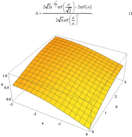
(10) In the following Figure 1, the mean difference Δ is shown on vertical axis de-pending on the minimum value a and the maximum value b indicated on base axes.As can easily be seen, starting from 0, when a and b are both zeros, the mean difference grows with a decreasing and b increasing up to the maximum, equal to 2
π, which is obtained when a = −∞ and b = ∞ , that is the case of com-plete normal distribution.
4. Special Cases
Let us consider mean difference formulas in some interesting special cases of truncated normal distribution.
4.1. Symmetric Truncated Distribution
When b= −a in the general formula, after a few steps it leads to
( )
2 2 2 2 2e erf 2erf 2 . 2 erf a a a a − − ∆ = π π (11)DOI: 10.4236/am.2020.1111078 1165 Applied Mathematics
4.2. Truncated Semi-Normal Distribution
When a =0 in the general formula, after a few steps it leads to
( )
22 2 2erf 2erf 1 e 2 . 2 erf 2 b b b b − − + ∆ = π (12) When b =0, it leads to a similar result( )
2 2 2 2erf 1 e 2erf 2 . 2 erf 2 a a a a − + − ∆ = π (13)4.3. Semi-Normal Distribution
When a =0 and b = ∞ in the general formula, after a few steps it leads to
(
)
2 2 2 . − ∆ = π (14) The same result is obtained when a = −∞ and b =0.4.4. Tail Normal Distribution
When a >0 and b = ∞ in the general formula, after a few steps it leads to
( )
2 2 2 4 1 erf 2 2e 1 erf 2 . 1 erf 2 a a a a − − − − ∆ = π − (15) The same result is obtained with a = −∞ and b <0 in the general formula:( )
2 2 2 4 1 erf 2e 1 erf 2 . 1 erf 2 b b b b − + − + ∆ = π + (16)4.5. Complete Normal Distribution
When a = −∞ and b = ∞ , it leads to the well-known result of mean difference of complete normal distribution.
2 . ∆ =
π (17) In this work, we do not deal with other special cases.
5. Conclusion
DOI: 10.4236/am.2020.1111078 1166 Applied Mathematics applied in many experimental and observational fields, particularly in quantita-tive economic sciences. Variability indexes as range of variation, mean deviation and standard deviation and shape indexes (asymmetry and disnormality) have been already obtained, but the mean difference of the truncated normal distribu-tion is not known in literature. This note fills the gap regarding the lack of knowledge of mean difference general formula of said model. Moreover, the ob-tained formula is proposed for any truncation and for some particular truncated cases.
Conflicts of Interest
The authors declare no conflicts of interest regarding the publication of this pa-per.
References
[1] Johnson, N.L., Kotz, S. and Balakrishnan, N. (1994) Continuous Univariate Distri-butions. Wiley, New York, Vol. 1, Cap. 10, Par. 1.
[2] Hamedani, G.G. (2019) Characterizations of Recently Introduced Univariate Con-tinuous Distributions II. Nova Science Publishers, New York.
[3] Barr, D.R. and Sherrill, E.T. (1999) Mean and Variance of Truncated Normal Dis-tributions. The American Statistician, 53, 357-361.
https://doi.org/10.1080/00031305.1999.10474490
[4] Domma, F. (2003) Informazione di Fisher e modellitroncati. Statistica, 63, 267-284. [5] Cha, J., Cho, B.R. and Sharp, J.L. (2013) Rethinking the Truncated Normal Distri-bution. International Journal of Experimental Design and Process Optimisation, 3, 27-63. https://doi.org/10.1504/IJEDPO.2013.059667
[6] Koutroumbas, K.D., Themelis, K.E. and Rontogiannis, A.A. (2014) Approximating the Mean of a Truncated Normal Distribution, Cornell University.
[7] Thomopoulos, N.T. (2015) Standard Normal and Truncated Normal Distributions. In: Demand Forecasting for Inventory Control, Springer International Publishing, New York, 137-148.
https://doi.org/10.1007/978-3-319-11976-2_10
[8] Domma, F. and Hamedani, G.G. (2014) Characterizations of a Class of Distribu-tions by Dual Generalized Order Statistics and Truncated Moments. Journal of Sta-tistical Theory and Applications, 13, 222-234.