DOTTORATO DI RICERCA IN INGEGNERIA
MECCANICA E INDUSTRIALE
XXXIII CICLO
Settore concorsuale ING-IND/14
N
UMERICAL AND
S
EMI
-
ANALYTICAL
M
ODELS
A
PPLIED TO
W
HEEL
-R
AIL
C
ONTACT
P
ROBLEMS
R
ELATORE
P
ROF
.
A
NGELO
M
AZZÙ
C
OORDINATRICE
P
ROF
.
SSA
L
AURA
E
LEONORA
D
EPERO
D
OTTORANDO
DOTTORATO DI RICERCA IN
INGEGNERIA MECCANICA E INDUSTRIALE
Settore scientifico disciplinare ING-IND/14
CICLO XXXIII
NUMERICAL AND SEMI-ANALYTICAL MODELS APPLIED TO
WHEEL-RAIL CONTACT PROBLEMS
Dottorando:
Ing. Nicola Zani
Relatore:
Prof. Angelo Mazzù
Coordinatore:
Table of contents
List of figures
IV
List of tables
IX
Abstract
1
PART I
Chapter 1 - Introduction
1.1
Rail transport
3
1.2
Thesis structure
9
1.3
References
10
Chapter 2 - Review of wheel/rail materials and damage
phenomena
2.1
Wheel materials
11
2.2
Rail materials
13
2.3
Phenomena in the wheel–rail interface
14
2.4
References
20
PART II
Chapter 3 - Effect of solid contaminants on wheel/rail
material couplings
3.1
State of the art and motivation
25
3.3
Results
32
3.4
Comparison with experimental results
44
3.5
Concluding remarks
46
3.6
References
47
PART III
Chapter 4 - Effect of traces of bainite in railway wheels
4.1
State of the art and motivation
53
4.2
Experimental evidence
57
4.3
Model of analysis
59
4.4
Semi-analytical model results (SAM)
65
4.5
Finite Element model results (FEM)
66
4.6
Discussion of the results
75
4.7
Concluding remarks
76
4.8
References
77
PART IV
Introduction to the semi-analytical model
85
Chapter 5 - Contact mechanics
5.1
Hertzian theory
87
5.2
Distributed normal and tangential tractions
91
5.3
Post-processing
93
5.4
References
95
Chapter 6 - Constitutive models
6.1
Some notes on tensor calculus
97
6.2
General remarks on constitutive modelling
100
6.3
Plasticity
100
6.4
Chaboche plastic model
105
6.5
References
108
Chapter 7 - Multixial fatigue criteria
7.1
High cycle fatigue criteria
111
7.2
Low cycle fatigue criteria
114
7.4
References
116
Chapter 8 - Wear
8.1
Modelling wear
118
8.2
References
119
Chapter 9 - Simulations
9.1
Hertzian contact and elastic stress quantities
120
9.2
Cyclic plasticity
138
9.3
Convergence in the wear model
144
9.4
Multiaxial fatigue: Dang Van and Crossland
145
9.5
Multiaxial fatigue: Jiang-Sehitoglu
147
9.6
Conclusions and ongoing activities
149
9.7
References
150
Chapter 10 - Conclusions and perspctives
10.1 Conclusions
153
List of figures
PART I
Chapter 1 - Introduction
Figure 1.1 – Route length (km) in European countries participating in the
survey in 2018 6
Figure 1.2 – Top speed train records and maximum operating speeds (Maglev
trains are not considered) 7
Chapter 2 - Review of wheel/rail materials and damage
phenomena
Figure 2.1 – Regions of contact between the rail head and wheel flange (1) 15 Figure 2.2 – Wear map BS11 rail steel versus AAR CLASS D (7) 16
Figure 2.3 – Example of T𝛾 approach plot (5) 16
Figure 2.4 – Different types of contact loading and resulting crack formation 17 Figure 2.5 – Shelling in a railway wheel (courtesy of Lucchini RS) 17 Figure 2.6 – Micrographs showing shelling in railway wheels (courtesy of
Lucchini RS) 18
Figure 2.7 – Surface-initiated RCF causing surface pitting (8) 18 Figure 2.8 – Thermal cracks extending in an axial/radial direction (8) 19 Figure 2.9 – Material response to cyclic loading (σ is stress, ε is the deformation)
20 Figure 2.10 – Shakedown map defined by current friction force and normalised
contact pressure (5) 20
PART II
Chapter 3 - Effect of solid contaminants on wheel/rail material
couplings
Figure 3.2 – Finite element model of the clean contact 29 Figure 3.3 – Correlation between cyclic yield strength and Brinell hardness in
rail and wheel steels 30
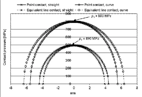
Figure 3.4 – Equivalent line contact pressure distributions compared with correspondent point contact distributions along the longitudinal axis of the
contact ellipse (22) 31
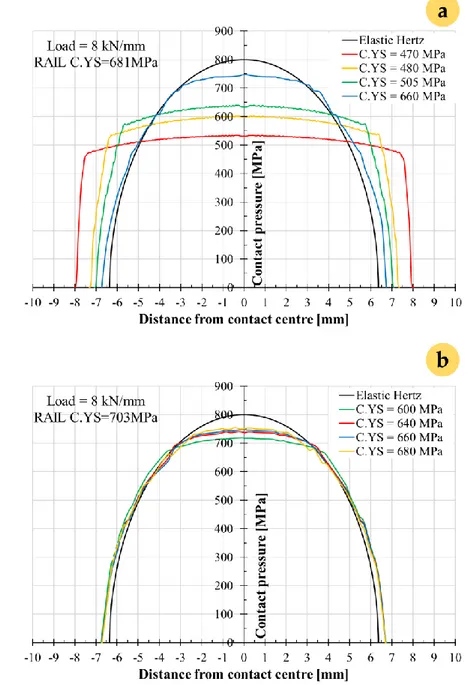
Figure 3.5 – Pressure distribution in clean contact in compression loading, with P = 8 kN/mm (curve condition): a) European couplings; b) American couplings
32 Figure 3.6 – Pressure distribution in contaminated contact, with P = 3 kN/mm
(a) and P = 8 kN/mm (b) 33
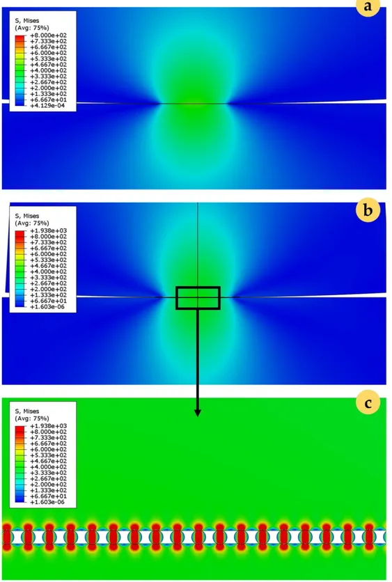
Figure 3.7 - Pressure distribution in clean contact in rolling condition with P = 8 kN/mm (curve condition): a) European couplings; b) American couplings 34 Figure 3.8 – Map of the Mises equivalent plastic strain in the contact zone with rail 𝐶. 𝑌𝑆𝑅 = 685 𝑀𝑃𝑎, wheel 𝐶. 𝑌𝑆𝑊 = 505 𝑀𝑃𝑎, p0 = 490 MPa in clean (a) and
contaminated contact (b,c) 35
Figure 3.9 – Map of the Mises equivalent plastic strain in the contact zone with rail 𝐶. 𝑌𝑆𝑅 = 685 𝑀𝑃𝑎 , wheel 𝐶. 𝑌𝑆𝑊 = 505 𝑀𝑃𝑎 , p0 = 490 MPa in clean contact: (a) compressive loading; (b) rolling condition 36 Figure 3.10 – Maximum von Mises equivalent plastic strain in clean contact in curve (p0 = 800 MPa) and in straight line (p0 = 490 MPa) as a function of the wheel cyclic yield strength 𝐶. 𝑌𝑆𝑊 for various rail cyclic yield strength 𝐶. 𝑌𝑆𝑅
in: a) wheels; b) rails 37
Figure 3.11 – Maximum von Mises plastic strain p Mises in contaminated contact in curve (p0 = 800 MPa) and in straight line (p0 = 490 MPa) as a function of the wheel cyclic yield strength 𝐶. 𝑌𝑆𝑊 for various values of the rail cyclic yield
strength 𝐶. 𝑌𝑆𝑅; a) in wheels; b) in rails 38
Figure 3.12 – Maximum von Mises equivalent plastic strain in clean contact in rolling condition in curve (p0 = 800 MPa) and in straight line (p0 = 490 MPa) as a function of the wheel cyclic yield strength 𝐶. 𝑌𝑆𝑊 for various rail cyclic yield
strength 𝐶. 𝑌𝑆𝑅 in: a) wheels; b) rails 39
Figure 3.13 – Von Mises equivalent plastic strain in contaminated contact in straight line (p0 = 490 MPa) as a function of the wheel cyclic yield strength 𝐶. 𝑌𝑆𝑊 for various rail cyclic yield strength 𝐶. 𝑌𝑆𝑅 in wheels: a) wheels; b) rails
40 Figure 3.14 – Von Mises equivalent plastic strain in contaminated contact in curve (p0 = 800 MPa) as a function of the wheel cyclic yield strength 𝐶. 𝑌𝑆𝑊for various rail cyclic yield strength 𝐶. 𝑌𝑆𝑅 in rails: a) wheel; b) rail 41 Figure 3.15 – Gradient of the Mises stress below the location of the particle closest to the contact centre, with rail 𝐶. 𝑌𝑆𝑅 = 489 𝑀𝑃𝑎 , wheel 𝐶. 𝑌𝑆𝑊 = 505 𝑀𝑃𝑎, p0 = 490 MPa; a) overall; b) zoom on layer with z < 0.2 mm 42 Figure 3.16 – Variation of the depth of influence of the local particle-body contact normalized with the particle radius as a function of the wheel 𝐶. 𝑌𝑆𝑊, for various rail 𝐶. 𝑌𝑆𝑅 and contact pressure, compared with the case of fully
elastic materials: a) in wheels; b) in rails 43
Figure 3.17 – Micrographs of the sections of wheel and rail steels tested in (2) in clean condition: a) EN ER8 wheel steel (𝐶. 𝑌𝑆𝑊 = 470 𝑀𝑃𝑎); b) R350HT rail steel (𝐶. 𝑌𝑆𝑅 = 691 𝑀𝑃𝑎), tested against the EN ER8; c) SANDLOS® S wheel steel (𝐶. 𝑌𝑆𝑊 = 660 𝑀𝑃𝑎); d) R350HT rail steel tested against the SANDLOS®
Figure 3.18 – Micrographs of the sections of wheel and rail steels tested in (2) in sand contaminated condition: a) EN ER8 wheel steel 𝐶. 𝑌𝑆𝑊); b) R350HT rail steel (𝐶. 𝑌𝑆𝑅 = 691 𝑀𝑃𝑎), tested against the EN ER8; c) SANDLOS® S wheel steel (𝐶. 𝑌𝑆𝑊 = 660 𝑀𝑃𝑎); d) R350HT rail steel, tested against the SANDLOS®
S 45
PART III
Chapter 4 - Effect of traces of bainite in railway wheels
Figure 4.1 – Location of the specimens analysed to calculate the bainitic spots
dimensions (unit: mm) 57
Figure 4.2 – Equivalent radius” distribution in six railway wheels 58 Figure 4.3 – Micrographs showing the bainitic structure in the ferritic-pearlitic
matrix with different amount of bainitic spots: 58
Figure 4.4 – Semi-analytical model used for the comparison with SAM 62 Figure 4.5 – Finite element model used for the comparison with SAM 63 Figure 4.6 – Stress-strain curves for Swift and Ramberg-Osgood constitutive
laws 63
Figure 4.7 – Von Mises stress along the depth at the centre of the contact in
presence of a circular inhomogeneity 64
Figure 4.8 – Plastic strain along the depth at the centre of the contact in presence
of a circular inhomogeneity 64
Figure 4.9 – a) Rolling contact problem in SAM, b) Von Mises stress field in the rolling
plane when the contact load is above the cluster of bainite 65 Figure 4.10 – Von Mises stress profile in presence of three phases along the
depth varying the radius dimension 66
Figure 4.11 – Finite element model: on the right, the global model; on the left,
the sub-model 67
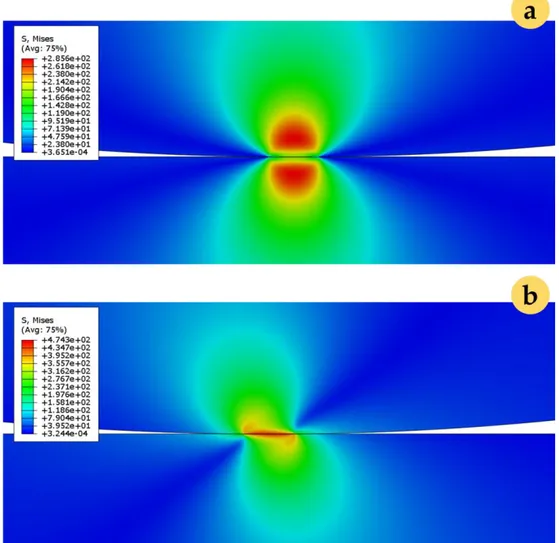
(below) Figure 4.12 – Von Mises plastic strain distribution around the bainitic
spots according to phase size (z/a = 0.78) 69
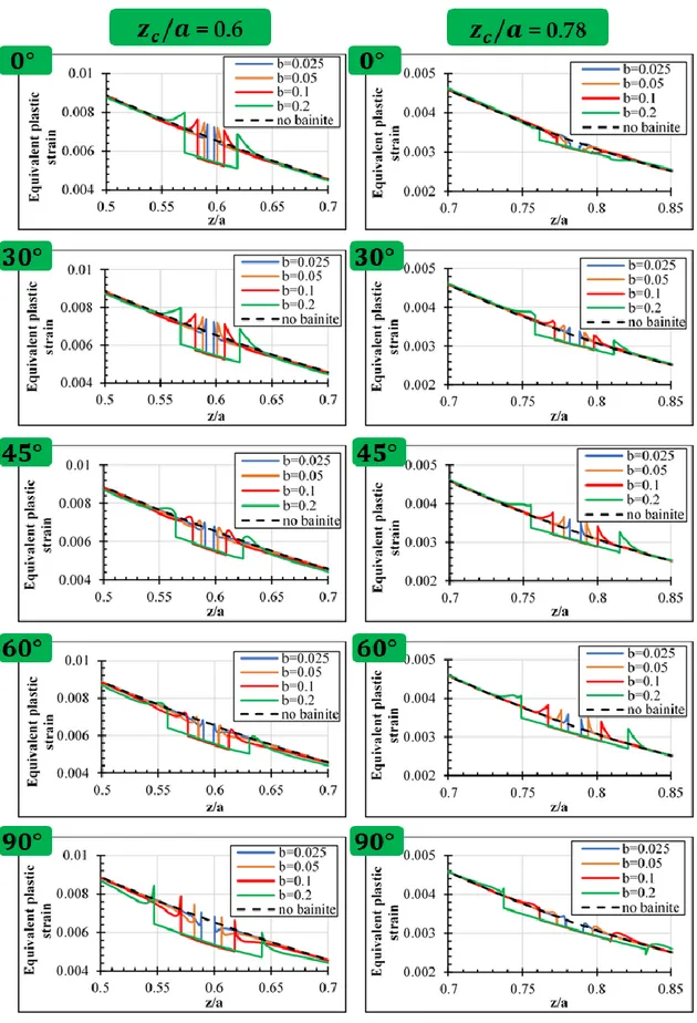
Figure 4.13 – Von Mises equivalent plastic strain evolution according to radius dimensions after one cycle: (a) circular bainitic spots centred at 2.5 mm depth (z/a =0.6); (b) circular bainitic spots centred at 3.3 mm (z/a = 0.78) 69 Figure 4.14 – Von Mises equivalent plastic strain profile according to ellipse dimension, major axis inclination and depth after one cycle loading (b = major
semi-axis in mm) 71
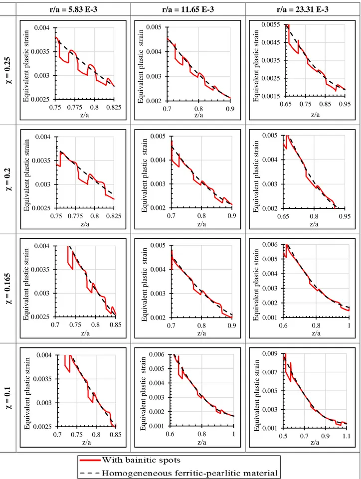
Figure 4.15 – Residual equivalent von Mises plastic strain (PEEQ) according to axis bainitic phase slope (major axis set to 100 μm) 72 Figure 4.16 – Plastic strain profile after one cycle loading for circular section bainite spots according to different interaxis and radius 74
PART IV
Chapter 5 - Contact mechanics
Figure 5.1 – Schematic representation of the cylindrical (line) contact 90 Figure 5.2 – Elastic half-space loaded by a normal pressure p(x) and a tangential
traction distributed in an arbitrary manner 91
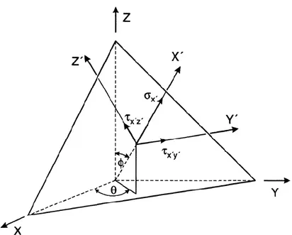
Figure 5.3 – Stresses acting on a plane in a three-dimensional coordinate system 94
Figure 5.4 – Rotating coordinate system in the half-space model 94
Chapter 6 - Constitutive models
Figure 6.1 – Types of constitutive models 101
Figure 6.2 – Basic elastic-plastic response in uniaxial case 102 Figure 6.3 – Isotropic hardening: deviatoric plane and stress-strain curve
(linear hardening) 104
Figure 6.4 – Kinematic hardening: deviatoric plane and stress-strain curve
(linear hardening) 104
Figure 6.5 – Mixed hardening: deviatoric plane and stress-strain curve (linear
hardening) 104
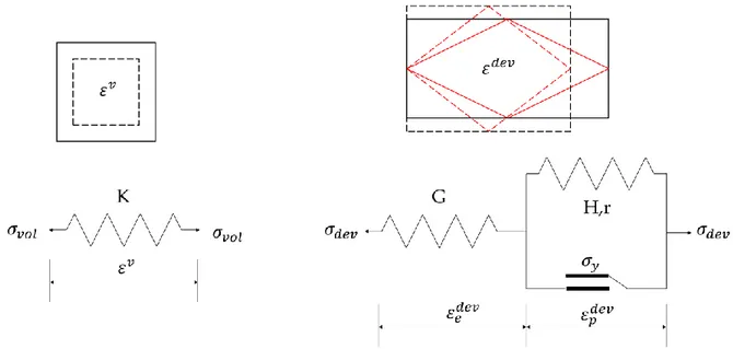
Figure 6.6 – Stress-strain curve for mixed non-linear hardening 104 Figure 6.7 – Rheological model for multiaxial plastic with hardening 105
Chapter 7 - Multixial fatigue criteria
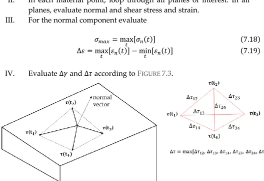
Figure 7.1 – Normal stress and shear stress acting on a material plane. O is the
application point of the vector t 113
Figure 7.2 – Definition of shear strain amplitude through the construction of
the minimum circumscribed circle to curve 𝛹 113
Figure 7.3 – Evaluation of shear stress range Δτ . Example with stresses evaluated at four instants in time. The shear strain range is evaluated in the
same way. 115
Chapter 9 - Simulations
Figure 9.1 – Schematic representation of the general and the line contact 121 Figure 9.2 – Hertzian pressure distribution in the line contact problem 122 Figure 9.3 – Hertzian pressure distribution in the elliptical contact problem: (a) contact loading in direction x in MPa; (b) contact loading in direction y in MPa;
(c) 3D pressure plot and contour plot. 123
Figure 9.4 – Elastic stresses and von Mises contours in the plane 𝑦 = 0 (friction coefficient 𝑓 = 0, 𝑝𝐻 = 1100 MPa (line contact)) 124 Figure 9. 5 – Principal stresses and deviatoric stresses contours in the plane 𝑦 = 0 (friction coefficient 𝑓 = 0, 𝑝𝐻 = 1100 MPa (line contact)) 125 Figure 9.6 – Elastic stresses and von Mises contours in the plane 𝑦 = 0 (friction coefficient 𝑓 = 0.3, 𝑝𝐻 = 1100 MPa (line contact)) 126 Figure 9.7 – Principal stresses and deviatoric stresses contours in the plane 𝑦 = 0 (friction coefficient 𝑓 = 0.3, 𝑝𝐻 = 1100 MPa (line contact)) 127 Figure 9.8 – Elastic stresses and von Mises contours in the plane 𝑦 = 0 (friction coefficient 𝑓 = 0.5, 𝑝𝐻 = 1100 MPa (line contact)) 128 Figure 9.9 – Principal stresses and deviatoric stresses contours in the plane 𝑦 = 0 (friction coefficient 𝑓 = 0.5, 𝑝𝐻 = 1100 MPa (line contact)) 129 Figure 9.10 – Elastic stresses and von Mises contours in the plane 𝑦 = 0 (friction coefficient 𝑓 = 0, 𝑝𝐻 = 1100 MPa (elliptical contact)) 130 Figure 9.11 – Principal stresses and deviatoric stresses contours in the plane 𝑦 = 0 (friction coefficient 𝑓 = 0, 𝑝𝐻 = 1100 MPa (elliptical contact)) 131 Figure 9.12 – Elastic stresses and von Mises contours in the plane 𝑦 = 0 (friction coefficient 𝑓 = 0.3, 𝑝𝐻 = 1100 MPa (elliptical contact)) 132 Figure 9.13 – Principal stresses and deviatoric stresses contours in the plane 𝑦 = 0 (friction coefficient 𝑓 = 0.3, 𝑝𝐻 = 1100 MPa (elliptical contact)) 133
Figure 9.14 – Elastic stresses and von Mises contours in the plane 𝑦 = 0 (friction coefficient 𝑓 = 0.5, 𝑝𝐻 = 1100 MPa (elliptical contact)) 134 Figure 9.15 – Principal stresses and deviatoric stresses contours in the plane 𝑦 = 0 (friction coefficient 𝑓 = 0.5, 𝑝𝐻 = 1100 MPa (elliptical contact) 135 Figure 9.16 – Elastic stresses along the rolling direction x at 𝑧𝑎 = 0.15 and 𝑧𝑎 =
0.5 (line contact) 136
Figure 9.17 – Elastic stresses along the rolling direction x at 𝑧𝑎 = 0.15 and 𝑧𝑎 = 0.5
(elliptical contact) 137
Figure 9.18 – Shear plastic strain versus number of cycles (left) and dimensionless depth z/a (right) according to the friction coefficient 139 Figure 9.19 – Shear plastic stain versus number of cycles according to the
geometry contact type 140
Figure 9.20 – Shear plastic strain versus number of cycles and dimensionless depth z/a according to the contact pressure (1100 MPa on the left, 1800 MPa on the right) when the friction coefficient is set to 0.3 141 Figure 9.21 – Shear plastic strain versus number of cycles and dimensionless depth z/a according to the contact pressure (1100 MPa on the left, 1800 MPa on the right) when the friction coefficient is set to 0.5 142 Figure 9.22 – (following page) Shear plastic strain versus number of with and without the effect of wear. The first row refers to contact pressure equal to 1100
MPa, the second one to 1800 MPa 143
Figure 9.23 – Schematic representation of the layers 144 Figure 9.24 – Shear plastic strain along the depth according to different ∆𝑧 size
144 Figure 9.25 – Dang Van and Crossland equivalent stress according to the dimensionless depth z/a for line and elliptical contact 146 Figure 9.26 – Plastic shear strain evolution at four depths 147 Figure 9.27 – 𝛥𝜏, 𝛥𝛾 and FP parameter by varying the depth and the angle 𝜗 148
List of tables
PART I
Chapter 2 – Review of wheel/rail materials and damage
phenomena
Table 2.1 – (top) Minimum and maximum content of the alloy elements in European and American steel grades, according to EN 13262 and AAR M-107/M-208 codes; (bottom) common applications of AAR and ER wheel steel
grades (1) 12
Table 2.2 – Typical rail steel grades in Europe, according to EN 13674-1:2009
(1) 13
Table 2.3 – Main rail steel grades in the USA (1) 14
PART II
Chapter 3 - Effect of solid contaminants on wheel/rail material
couplings
Table 3.1 – Main steel grades for wheel/rail couplings used in Europe (above)
and America (below) in straight line and curve 26
Table 3.2 – Main mechanical properties for improved UPLOS® and SANDLOS® family steels.UPLOS® A.CL.C and UPLOS® A.CL.D are the steel grades developed by Lucchini RS in compliance with AAR standards 27
PART III
Chapter 4 - Effect of traces of bainite in railway wheels
Table 4.1 – Mechanical properties for MICRALOS and AAR C wheel steels (23) 55 Table 4.2 – Mechanical properties for ER7 (ferritic-pearlitic steel) and HYPERLOS® (ferritic-pearlitic with traces of bainite) (29) 56 Table 4.3 – Details about the semi-analytic and the finite element models
adopted for the comparison 60
Table 4.4 – Mechanical properties for materials employed in the simulations
for FEM and SAM comparison 62
Table 4.5 – Details about the FE model and computing time 68 Table 4.6 – Plastic properties of the bainitic spots in FEM simulations 68
Table 4.7 – Interaxis adopted with respect to bainite size according to different
radius dimension 73
Table 4.8 – Average amount of bainitic phases according to different radius
dimension 73
PART IV
Chapter 9 - Simulations
Table 9.1 – Geometrical properties of the adopted models. elastic properties
and results of the Hertzian problem 121
Table 9.2 – Plastic properties of the material (1) 138 Table 9.3 – Multiaxial fatigue material parameters 145 Table 9.4 – Von Mises shear stress threshold for elastic response according to
Abstract
La presente tesi, sviluppata in collaborazione con l’azienda Lucchini RS (Lovere, Italia), è incentrata sullo sviluppo di modelli numerici e semi-numerici per applicazioni ferroviarie, in particolare il contatto ruota-rotaia. Tre diverse aree di ricerca sono oggetto di analisi.
La prima di queste riguarda lo studio dell’effetto di contaminanti solidi interposti tra la ruota e la rotaia, come per esempio la sabbia negli ambienti desertici. Nonostante in particolari circostanze la sabbia venga utilizzata per migliorare l’adesione tra ruota e rotaia, i granelli di sabbia così come i detriti di rocce possono drammaticamente peggiorare il comportamento ad usura; inoltre, le pressioni localizzate sui componenti sono fonte di deformazioni plastiche di intensità maggiore rispetto ad un contatto asciutto. Il corretto abbinamento dei materiali di ruote e rotaie risulta di fondamentale importanza per migliorare l’efficienza e la vita utile di questi componenti. Simulazioni numeriche agli elementi finiti sono state eseguite per valutare come il campo delle deformazioni plastiche cambia al variare dell’accoppiamento dei materiali.
Il secondo tema trattato è di natura metallurgica e riguarda la microstruttura delle ruote monoblocco. La microstruttura è tipicamente ferritico-perlitica e tale struttura rimane la migliore dal punto di vista della resistenza ad usura e a fatica. Tuttavia, la formazione della bainite è inevitabile durante il raffreddamento continuo degli acciai ipoeutettoidici e la presenza di bainite potrebbe compromettere il comportamento meccanico della ruota, poiché la bainite presenta una velocità di usura maggiore della perlite. Inoltre, è risaputo che fasi metallurgiche di diversa natura vicine tra loro possono generare sovrasollecitazioni e, di conseguenza, maggiori deformazioni a causa delle diverse delle proprietà meccaniche. Lucchini RS ha individuato la velocità di raffreddamento da adottare durante il trattamento termico di rim chilling che permette di contenere il più possibile le tracce di isole bainitiche nella corona di rotolamento della ruota e di ottenere la durezza e la tenacità richiesta dalle normative. Obiettivo di questa tesi è individuare la massima quantità di isole bainitiche nella microstruttura ferritico-perlitica che non compromette il comportamento della ruota dal punto di vista della deformazione plastica. Per raggiungere
questo obiettivo, si è ricorso a modelli numerici agli elementi finiti e ad un modello semi-analitico scritto dai ricercatori francesi dell’Institute National
des Sciences Appliquées di Lione (INSA-Lyon).
Nella terza parte viene proposto un modello semi-analitico, mirato a risolvere problemi di contatto non conforme, come quello ruota-rotaia. L’utilizzo di un modello semi-analitico anziché uno numerico presenta come principale vantaggio la riduzione del tempo di calcolo. Il modello si propone principalmente di trovare la risposta ciclica del materiale, partendo dalla risoluzione del problema del contatto Hertziano, dal calcolo del campo degli sforzi elastici e dal modello costitutivo plastico di Chaboche. Infine, sono proposti alcuni criteri di verifica a fatica multiassiale ad alto e basso numero di cicli. Questa parte è stata realizzata in collaborazione con la
Chalmers University of Technology di Göteborg in Svezia.
Parole chiave: teoria del contatto non conforme, metodo agli elementi finiti, modello semi-analitico, contaminanti solidi, fatica per contatto ciclico, fatica ad alto/basso numero di cicli, usura, deformazioni plastiche, microstruttura, bainiti.
Key words: non-conforming contact mechanics theory, finite element models, semi-analytical models, solid contaminants, rolling contact fatigue, high/low cycles fatigue, wear, plastic deformation, microstructure, bainite.
Chapter 1 - Introduction
Chapter 2 - Review of wheel/rail
materials and damage phenomena
I
Part I
Introduction
1.1 Rail transport
The railway is considered a means of fast and secure transportation. The constant development of this sector has led to an improvement in the performance of rail transport; nevertheless, this does not prevent conditions limiting the optimum efficiency and performance.
Railway transport has comparative advantages (noticeably, speed and comfort for passengers and economies of scale for freight) with medium to long distances over other means of transportation. According to the
Independent Regulators Group – Rail (IRG-Rail), the route length for the
monitored European countries is over 234,000 km (1). Furthermore, over 50% of this total is from only five countries: Italy, Germany, France, Poland and the United Kingdom. FIGURE 1.1 illustrates the route length in 2018. Across the countries that participated in the IGR-Rail survey in 2018, 55% of the total route is electrified. Since 2014, the length of electrified tracks has been slowly increasing at an average rate of 0.6% per year. On the other hand, the non-electrified route tracks have been decreasing since 2014 by about 0.7% (1).
If we focus on the European rail traffic from 2014 to 2018, the rate of distribution between passenger and freight has been substantially unchanged. Over a total of 4.5 billion train-km reported, freight traffic only contributed 19%, while passenger traffic accounted for the remaining 81%. The difference in freight and passenger traffic volumes is due to the rail freight services suffering from reliability and low quality, as a result of the lack of traffic management and the absence of coordination in the cross-border capacity (2).
The situation in the United States of America (USA) differs completely, where freight traffic is more diffused than passenger services. USA had about 222,900 railroad route-km in 2017 (1), whereas the route length of passenger rails service operated over about 34,500 km. The next chapter elaborates on how this opposite trend with respect to Europe implies a different choice in the railway wheels material.
The history of the wheel–rail systems has mirrored the industrial revolution started in the second half of the 18th century and the technological advances achieved. Flanged wheels running on a cast-iron rail have been in use since the 18th century. Coned wheels with a flangeway clearance, enabling the wheels to run on a straight track without flange–rail contact, were established in the 1830s. The spread of the industrial revolution throughout Europe in the first half of the 19th century lead to massive railway projects. In 1825, the first railway line with locomotives and regular traffic opened in England. A decade later, the first Italian train line was launched.
The maximum speed has been increasing over the years. In 1830, the Rocket steam locomotive designed by Robert Stephenson reached a speed of approximately 50 km/h. In 1903, Siemens & Halske designed the first experimental electric rail car, which exceeded 200 km/h.
The 1960s saw a rise in high-speed trains. In 1964, the Japanese Shinkansen, or bullet train, was introduced, travelling at a maximum speed of 210 km/h. In 1981, the French TGV (Train à Grande Vitesse) was introduced at 260 km/h and now runs at 300–320 km/h in regular traffic. FIGURE 1.2 shows the
maximum operating speed and top speed records of trains worldwide (3).
Figure 1.1 – Route length
(km) in European countries participating in the survey in 2018
Unlike the conventional trains that use wheels, the Maglev train is based on magnetic levitation. This kind of train is costly to construct, with only three operational Maglev systems in existence, in South Korea, China and Japan. The Chinese Maglev has the highest run speed of 431 km/h, while, in 2015, the Japanese Maglev hit a record of 603 km/h.
Axle loads have been increasing significantly over the years, reaching values of 30, 35 and 40 tonnes per axle for heavy-haul applications (especially in the USA and Australia).
Figure 1.2 – Top speed
train records and maximum operating speeds (Maglev trains are not considered)
Figure 1.3 – A short description of Lucchini RS company;
1.2 Thesis structure
The trend to heavier axle loads and higher speeds has increased the demand for more defined mechanical properties and geometries. Inefficiently designed railway components (rails, wheels, axles, etc.) and materials can lead to a dramatic increase in maintenance costs, train delays and personal injuries. The optimal design may even contribute to reducing CO2 emissions and energy consumption. With this goal in mind, many railway companies and universities have been carrying out research activities in this field. This thesis was financed by the Lucchini RS company, and it examines some railway challenges from a numerical point of view using finite element methods (FEM) and semi-analytical models. FEM models were carried out with the commercial software Abaqus®. The current work contains four parts.
Part 1 includes this introductory chapter (Chapter 1) and Chapter 2. The first
section of Chapter 2 gives a brief overview of the wheel and rail steels, focusing on European and American materials. In addition, the main phenomena occurring at the wheel-rail interface are proposed: contact, wear and fatigue.
Part 2 examines the effect of solid contaminants in wheel–rail contact
(Chapter 3). After a short literature review about this topic, the finite element models are illustrated. The main task of this chapter is to investigate how the changing of wheel and rail material couplings influences the plastic deformation in wheels and rails. The numerical results are then compared to the experimental outcomes obtained through a twin-disk testing machine. The effect of non-homogeneous microstructure in railway wheels is analysed in Part 3. Chapter 4 first illustrates the possible microstructures of railway wheels (ferritic-pearlitic, bainitic and ferritic-pearlitic with traces of bainite), highlighting the qualities and the defects of each alternative. Numerical models and semi-analytical models will be proposed to study the effect of small traces of bainite in ferritic-pearlitic wheel steels. Determining the amount of bainite that does not compromise wheel behaviour is the goal. This chapter was carried out in partnership with the French university INSA-Lyon.
Part 4 is concerned with a semi-analytical model coded in Matlab®, whose aim is to investigate the cyclic response in non-conformal contact problems. This part is organised in four theoretical chapters and the final chapter illustrating the results. Chapter 5 explains the contact mechanics theory, focusing on the Hertzian theory applied to cylindrical and elliptical contact.
Chapter 6 shows how to solve the elastic problem to obtain the elastic stress
of the bodies in contact. The plastic constitutive law is presented in Chapter
7. Chapter 8 shows how wear is handled in the model. Lastly, Chapter 9
analyses the results of the simulations. This part was carried out in partnership with Chalmers University of Technology in Gotheborg (Sweden).
1.3 References
1. Independent Regulators Group – Rail. Eight annual market monitoring report, Mar 2020. https://www.irg-rail.eu/irg/documents/market-monitoring/260,2020.html
2. Transport in the European Union, Current Trends and Issues, Mar 2019.
https://ec.europa.eu/transport/sites/transport/files/2019-transport-in-the-eu-current-trends-and-issues.pdf
3. U.S. Department of Transportation. Transport statistics annual report 2018. https://www.bts.gov/sites/bts.dot.gov/files/docs/browse- statistical-products-and-data/transportation-statistics-annual-reports/TSAR-Full-2018-Web-Final.pdf 4. https://www.statista.com/chart/10792/the-worlds-fastest-high-speed-trains/ 5. https://lucchinirs.com/portfolio/residual-stress-measurement-on-wheels-and-axles/
Review of wheel–rail
materials and damage
phenomena
2.1 Wheel materials
The traditional approach to railway solid-wheel materials uses carbon steel for almost every application; however, the standards followed in North America (AAR), Russia (GOST), Japan (JIS) and Europe (EN) may vary. In this work, we only focus on EN and AAR.
According to EN 136262, the European solid wheels are mainly based on grade C steels, with carbon content in the range of 0.45–0.60%, lower than that of the North American solid wheels. For example, the C content of AAR Class B and C solid wheels ranges from 0.57 to 0.77%. Another main difference between the American and European chemical composition relies on the content of Si: the European range being lower (maximum 0.40%) compared to AAR range (0.15–1.00%). Si limits the formation of martensite and promotes the formation of pearlite. If pearlite formation is rapid, the austenite will form pearlite before it reaches the martensite transformation start temperature. The AAR standard also demands a calibrated content of sulfur to improve machinability; this requirement is rarely found in the European standards.
Solid wheels made of these materials can be produced in two main different heat treatment conditions: total quenching, that is rarely adopted, and rim chilling. The latter creates circumferential compressive residual stresses in the wheel rim, which suppress propagation of transverse cracks. Rim chilling also promotes a good combination of strength, toughness and resistance to wear.
TABLE 2.1shows the chemical composition of the European and American solid wheel steel grades and their common applications.
As previously stated, most solid wheels have been produced from carbon steel grades, with the appropriate content of Si and Mn. The resulting microstructure consists of two elements:
• soft ferrite generally generated around the prior austenite grain boundaries
• hard pearlite comprising lamellae of the softer ferrite and the harder cementite.
Table 2.1 – (top) Minimum and maximum content of the alloy elements in European and American steel
grades, according to EN 13262 and AAR M-107/M-208 codes; (bottom) common applications of AAR and ER wheel steel grades (1)
Grade Min. and max. content in European and North American steel grades (%)
C S P Mn Cr Ni Mo Cu Si V Al Nb Ti Cr+Ni+Mo EN ER6 Max 0.48 0.015 0.020 0.75 0.30 0.30 0.08 0.25 0.40 0.060 - - - 0.50 EN ER7 Max 0.52 0.015 0.020 0.80 0.30 0.30 0.08 0.25 0.40 0.060 - - - 0.50 EN ER8 Max 0.56 0.015 0.020 0.80 0.30 0.30 0.08 0.25 0.40 0.060 - - - 0.50 EN ERS8 Max 0.57 0.015 0.020 1.10 0.30 0.30 0.08 0.25 1.10 0.060 - - - 0.50 EN ER9 Max 0.60 0.015 0.020 0.80 0.30 0.30 0.08 0.25 0.40 0.060 - - - 0.50 AAR CLASS L Min - - - 0.60 - - - - 0.15 - - - - - Max 0.47 0.015 0.020 0.90 0.25 0.25 0.10 0.25 1.00 0.040 0.060 0.050 0.030 - AAR CLASS A Min 0.47 - - 0.60 - - - - 0.15 - - - - - Max 0.57 0.015 0.020 0.90 0.25 0.25 0.10 0.25 1.00 0.040 0.060 0.050 0.030 - AAR CLASS B Min 0.57 - - 0.60 - - - - 0.15 - - - - - Max 0.67 0.015 0.020 0.90 0.25 0.25 0.10 0.25 1.00 0.040 0.060 0.050 0.030 - AAR CLASS C Min 0.67 - - 0.60 - - - - 0.15 - - - - - Max 0.77 0.015 0.020 0.90 0.25 0.25 0.10 0.25 1.00 0.040 0.060 0.050 0.030 - AAR CLASS D Min 0.67 - - 0.60 - - - - 0.15 - - - - - Max 0.77 0.015 0.020 0.90 0.25 0.25 0.10 0.25 1.00 0.040 0.060 0.050 0.030 -
EN 13262 or AAR M107/M108 Common applications EN 13626 ER6
AAR CLASS L
Generally applied in low-axle load simulations, for some underground applications or regional and suburban passenger carriages and locomotives
EN 13626 ER7
Suitable for a wide range of applications in Europe, as it gives a good balance between toughness and hardness on the tread; mostly used for carriages and locomotives in passengers service
EN 13626 ER8
Commonly applied for heavy-duty applications; increasing demand in Europe in the last decade for applications requiring improved wheel wear, RCF (rolling contact fatigue) and out-of-roundness resistance
EN 13626 ER9 Seldom used in Europe, except for heavy-duty applications,
high-contact stress in special locomotives and carriages
AAR CLASS A
Rarely used in Europe, suitable for heavy-duty wheel application, high contact stress in special locomotives or rapid transit carriages
AAR CLASS B Seldom used in Europe, but very common in Japan and the USA mass transit transportation. Suitable for heavy-duty
applications, special suburban and urban vehicles, rapid transit carriages, heavily loaded locomotives with high diameter driving wheels with light braking conditions
AAR CLASS C
AAR CLASS D Suitable for locomotives and carriages under extreme load
and service conditions
This microstructure has shown an excellent combination of the mechanical properties required for the railway application. In these steels, the mechanical properties are mainly governed by the grain size, thickness of
the cementite lamellae and distance between the cementite lamellae. Fracture toughness, impact tests and area reduction are determined largely by the grain size and the thickness of the cementite lamellae. The mechanical properties improve when the thickness of the lamellae and the grain size decrease. Furthermore, when the interlamellar spacing decreases, the yield strength and the ultimate tensile stress increase.
The pearlitic microstructure can be altered in several ways, for example, by subjecting the steel to special heat treatment and accelerating cooling processes, changing the thickness of the lamellae, changing the proportion of the lamellae in the pearlite, precipitating fine carbides within the ferrite and so on. Increasing the content of C and introducing special alloying elements (Ni, Nb, V, Cr, Al, Ti and Mo) can alter the chemical composition. To achieve a sufficient level of toughness, pearlitic steels grades can be replaced with tempered bainitic and martensitic steel grades. These steels exhibit a different microstructure consisting of harder iron carbide laths embedded in softer acicular ferrite. Tempered bainitic martensitic steels are a good alternative to high-C steels when traditional requirements of microstructure and chemical analysis are not mandatory.
In Europe, forged solid wheels, or rolled tyres mounted on a wheel centre, are used almost exclusively. Manufacturing a forged railway wheel includes forging, rolling, heat treatment, machining and ultrasonic testing.
2.2 Rail materials
At present, most of the rail steels are made of carbon steel, with a C content ranging between 0.7 and 0.8%. The microstructure is typically pearlitic. EN13674-1:2011 is the European standard generally accepted by most railway companies. TABLE 2.2 shows the different options proposed in
Europe (2):
• standard carbon steel grade steels not heat-treated or “naturally cooled”
• alloyed rail steels not heat-treated or “naturally cooled” • traditional heat-treated rail steels
• R370CrHT and R400HT that are heat-treated steels with increased levels of hardness
Table 2.2 – Typical rail steel grades in Europe, according to EN 13674-1:2009 (1)
Rail steel grade
Hardness [HB]
Naturally cooled Heat-treated C, Mn steels Alloyed steels C, Mn steels Alloyed steels Ultra-high C R200 200–240 X R220 220–260 X R260 260–300 X R260Mn 260–300 X R320Cr 320–360 X (1% Cr) R350HT 350–390 X R350LHT 350–390 X R370CrHT 370–410 X R400HT 400–440 X
In North America, most rails comply with the AREMA (American Railway Engineering and Maintenance-of-Way Association) standard (TABLE 2.3). 25% are not heat-treated, while 75% are quenched and tempered.
Table 2.3 – Main rail steel grades in the USA (1)
Rail steel grade Hardness [HB]
AREMA 325 325–385 AREMA 370 370–410 AREMA 400 400–440
The heat-treated rail steels are beneficial for curves with radii less than 300 m or in unfavourable environmental conditions, like deserts. In the past twenty years, heat treatment has become a more standard product, especially in high normal axle load, in systems with very sharp curves, for heavy-haul applications and in turnouts. The heat treatment can be applied to the whole rail section or to a portion of the railhead.
Hyper-eutectoid steels have been recently produced as an improvement of the first eutectoid heat-treated carbon steels. The carbon level of these steels is roughly 0.8–0.9%, with a small addition of chromium, resulting in higher hardness values.
Similarly to wheels, pearlitic rails have been replaced by bainitic rails for applications that require higher yield strength, ultimate tensile strength, fracture toughness and hardness. Austenitic rails were manufactured as well.
Rails are produced from continuously cast blooms. During manufacturing, rails are checked for defects by automatic and continuous ultrasonic testing.
2.3 Phenomena in the wheel–rail interface
Wheel–rail contact is an extremely complex problem to solve that requires knowledge in various disciplines to understand and model. Furthermore, the lack of any analogies with other engineering components adds to the challenge. The main issue is the changing nature of the wheel–rail system: the continuous variations of the contact area and the stresses, which are different for each wheel, leading to different worn profiles. Another complexity of the wheel–rail contact is the fact that all the critical issues are interlinked. Consider, for example, rolling contact fatigue (RCF) and wear: if wear is reduced, cracks can grow to the point that RCF failure occurs; on the other hand, if crack growth is truncated, wear is more likely to be the problem. Friction modifiers are often used to control wear damage, but they may influence crack growth.
2.3.1 Wheel–rail contact
The position of the wheel–rail contact varies continuously as the train follows its path, with a typical contact patch of 1 cm2. The position depends on the wheel and rail profiles, the degree of curvature of the track and whether the wheel is the leading or trailing wheelset on a bogie. Three
possible regions can be identified (3,4). In straight track or high-radius curves, the railhead and wheel tread are likely to be in contact (Region A in
FIGURE 2.1), while the wheel flange and rail gauge corner will be in contact along tighter curves (Region B in FIGURE 2.1). The contact may also occur, but is least likely, between the field sides of the rail and wheel (Region C). In Region A, the lowest contact stresses and lateral forces occur; Region B yields to higher wear rates and contact stresses and two-point contacts may even occur; finally, Region C results in wear problems causing incorrect steering of the system.
Numerous mathematical solutions have been proposed over the years to solve the contact problem. The most straightforward approach was in the second half of the 19th century by Heinrich Hertz, considered the pioneer of the contact mechanics. Further details about his approach can be found in
CHAPTER 5.
2.3.2 Wear
Wear is the displacement or loss of material from a contacting surface. The wear mechanism depends on several factors, among which are the nature of the material and other elements of the tribo-system, including environmental conditions and the presence of other contaminants (sand, leaves, wear debris, friction modifiers, etc.) (4,5,6).
In wheel–rail contact, there are two areas of interest, sliding and rolling. Sliding motion (motion tangential to the surface) is more severe than motion perpendicular to the surface, occurring with rolling or impact. Sliding may result in oxidative wear in the mild contact condition (Region A, low sliding velocity and load) and in adhesive or galling wear (Region B). If particles are present in the contact, abrasive wear may also occur. In very severe sliding conditions, high heat generation may result in the contact leading to a thermal breakdown of the material.
Fatigue dominates the wear mechanisms during rolling motion. Typically referred to as fatigue wear, this kind of wear is created with the formation of cracks and separation of material due to repeated forces. These cracks seldom initiate below the surface and then propagate to the surface. However, if the traction force is significant, cracks initiate at the surface. Another critical kind of wear is abrasive wear, classified as three-body abrasive
wear when hard particles are trapped between the surfaces and two-body
Figure 2.1 – Regions of
contact between the rail head and wheel flange (1)
abrasive wear where the asperities of the harder body remove portions of the
softer body.
Wear is often classified as mild or severe. For any pair of materials, increasing either the normal load, sliding speed or temperature leads to a sudden jump in wear rate. Increasing temperature leads to the transition to a catastrophic wear regime. Mild wear results in smooth surfaces, and the debris is minimal (100 nm diameter), while severe wear in rough and torn surfaces has large debris (up to 0.01 mm diameter) (5). FIGURE 2.2(7) shows two example data from twin–disk testing using BS11 rail steel versus AAR CLASS D(data are available in (8)).
The most common wear models are the following:
• Archard model: It asserts that the wear volume V is directly proportional to the sliding distance l, the contact load P, but inversely proportional to the surface hardness H of the wearing material:
𝑉 = 𝑘𝑃 𝑙
𝐻 , (2.1)
where k is the wear coefficient
• 𝑇𝛾 approach: 𝑇 is the tractive force given by the normal force multiplied by the friction in the contact, and 𝛾 is the slip in the contact (FIGURE 2.3). This method is widely applied in the railway field.
Figure 2.3 – Example of T𝛾
approach plot (5)
Figure 2.2 – Wear map
BS11 rail steel versus AAR CLASS D (7)
2.3.3 Fatigue
RCF and wear are the main damage phenomena in rails and wheels. RCF is caused by cyclic loading of the material and results in cracks. These cracks can further propagate, causing the fracture of the component.
FIGURE 2.4 illustrates the crack formation and propagation that can occur
from contact loading under different conditions (9). FIGURE 2.4Ashows the case of pulsating vertical force, that can lead to surface or sub-surface cracks; in this case, the cracks will be arrested when they have grown out the contact stress zone (unless a bulk stress exists). In FIGURE 2.4B, the vertical
load (pulsating or constant) is combined with an oscillating lateral load (fretting fatigue), and cracks may form at the surface. In FIGURE 2.4C, the rolling condition is combined with interfacial shear and slip; this results in plastic deformation and crack initiation and growth.
Sub-surface–initiated rolling contact fatigue
Sub-surface–initiated RCF is relatively rare; however, when it occurs, it is potentially dangerous. The cracks initiate below the contact surface and, in the wheel, can branch towards the hub or the wheel surface (10). The crack formation is a result of low material resistance and high stress. Material cleanliness assumes a vital role since material defects may lead to intensified stresses (11,12). FIGURE 2.5 and FIGURE 2.6 illustrate examples of sub-surface–initiated RCF cracks in railway wheels.
Figure 2.4 – Different
types of contact loading and resulting crack formation
Figure 2.5 – Example of
sub-surface–initiated RCF in a railway wheel (courtesy of Lucchini RS)
Surface initiated rolling contact fatigue
Surface-initiated RCF cracks are more common but less severe than sub-surface ones. These cracks initiate because of frictional rolling/sliding contact leading to plastic deformation. The crack forms when plastic deformations exceed the plastic strain and propagate owing to the rolling contact loading and the hydro-pressurisation (caused by fluids trapped in the crack) (13). In wheels, surface-initiated cracks typically branch towards the surface and cause surface pitting (FIGURE 2.7), while cracks in rails may propagate downwards leading to transversal rail breaks.
Figure 2.7 – Surface-initiated RCF causing surface pitting (8) Figure 2.6 – Micrographs showing sub–surface RCF cracks in railway wheels (courtesy of Lucchini RS)
The remedy for surface cracks is re-profiling, which is a costly approach requiring trains to be taken out of traffic. Surface cracks may even be worn away by wear itself if slip is high enough; the balance between crack initiation and wear is referred to as the “magic wear rate” (14).
Thermal cracks
Thermal damage occurs when the outer layer of the wheel is severely heated (through the tread braking or, simply, the friction between wheel and rail). Thermal cracks initiate when the material plastically deforms from the restrained thermal expansion during heating; the tensile residual stresses induced by the cooling may promote crack propagation (15). Thermal damage is also related to material transformation. An example of thermal cracks in the wheels is shown inFIGURE 2.8.
Cyclic stress response
In general, four possible scenarios to cyclic response are known (FIGURE 2.9) (5,16):
• elastic response – no plastic deformation
• elastic shakedown – some plastic strains admitting in the early, but the material reverting to elastic behaviour owing to material hardening and residual stresses
• plastic shakedown – plastic strains following a hysteric cycle with no strain accumulation
• ratcheting – cyclic plastic strain accumulation
Figure 2.8 – Thermal cracks
extending in an axial/radial direction (8)
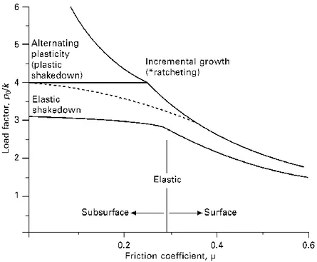
Shakedown maps are a useful tool to predict the cyclic response.FIGURE 2.10
(5) illustrates an example of a shakedown map for contact between coaxial cylinders; it shows the limit of the material behaviour in terms of the friction coefficient and a non-dimensional load factor, obtained by dividing the contact pressure by the shear yield strength. For friction coefficients above about 0.3, plastic flow is greatest on the surface.
2.4 References
1. Ghidini A, Diener M, Schneider J. Special wheels for mass transit, Lucchini RS, Lovere (Italy), 2014.
2. Ghidini A, Faccoli M., Mazzù A. SANDLOS® wheels for desert environments, Lucchini RS, Lovere (Italy), 2017.
Figure 2.9 – Material
response to cyclic loading (σ is stress, ε is the deformation)
Figure 2.10 – Shakedown
map defined by current friction force and normalised contact pressure (5)
3. Tournay, H., 2001, Supporting technologies vehicle track interaction, in Guidelines to Best Practice for Heavy Haul Railway Operations: Wheel and Rail Interface Issues, International Heavy Haul Association, Virginia Beach, VA, USA, 2-1-2.73.
4. Soleimani H, Moavenian M. Tribological Aspects of Wheel–Rail Contact: A Review of Wear Mechanisms and Effective Factors on Rolling Contact Fatigue. Urban Rail Transit 3, 227–237 (2017).
https://doi.org/10.1007/s40864-017-0072-2.
5. Lewis R, Olofsson U. Wheel-rail interface handbook, 1st edition. Woodhead Publishing Limited. September 2009. ISBN: 9781845694128. 6. Faccoli M, Petrogalli C, Lancini M, Ghidini A, Mazzù A. Effect of desert sand on wear and rolling contact fatigue behaviour of various railway wheel steels. Wear. 15 Feb 2018; 396–397:146–61.
https://doi.org/10.1016/j.wear.2017.05.012.
7. Lewis R, Olofsson U. Mapping rail wear regimes and transitions. Wear. Oct 2004; 257(7–8): 721–729. https://doi.org/10.1016/j.wear.2004.03.019. 8. Bolton PJ, Clayton P. Rolling–sliding wear damage in rail and tyre steels.
Wear. 16 Jan 1984; 92(2):145-165. https://doi.org/10.1016/0043-1648(84)90066-8.
9. Ekberg A, Åkesson B, Kabo E. Wheel/rail rolling contact fatigue – Probe, predict, prevent. Wear. 15 Jun 2014; 314(1–2):2–12.
https://doi.org/10.1016/j.wear.2013.12.004.
10. Ekberg A, Marais J. Effects of imperfections on fatigue initiation in railway wheels. Proc Inst Mech Eng Part F J Rail Rapid Transit. 2000; 214(1):45–54. https://doi.org/10.1243%2F0954409001531234.
11. Kabo E, Ekberg A. Material defects in rolling contact fatigue of railway wheels—the influence of defect size. Wear. 2005 Mar; 258(7–8):1194–200.
https://doi.org/10.1016/j.wear.2004.03.070.
12. Sandström J, De Maré J. Probability of subsurface fatigue initiation in rolling contact. Wear. 18 May 2011; 271(1–2):143–7.
https://doi.org/10.1016/j.wear.2010.10.018.ù
13. Mazzù A, Petrogalli C, Lancini M, Ghidini A, Faccoli M. Effect of Wear on Surface Crack Propagation in Rail–Wheel Wet Contact. J Mater Eng Perform. 2018 Feb 25; 27(2):630–9. https://doi.org/10.1007/s11665-018-3185-1.
14. Magel EE, Rolling Contact Fatigue: A Comprehensive Review, US Department of Transportation, Federal Railroad Administration, Technical Report, November 2011. http://www.fra.dot.gov/.
railway wheels: Towards experimental validation. Tribol Int. 2016 Feb 1; 94:409–20. https://doi.org/10.1177%2F0954409712452347.
16. Mazzù A. A simplified non-linear kinematic hardening model for ratchetting and wear assessment in rolling contact. J Strain Anal Eng Des. 2008; 43(5):349–60. https://doi.org/10.1243%2F03093247JSA405.
Chapter 3 - Effect of solid contaminants
on wheel/rail material couplings
(right image) Rail track in Namibia https://unsplash.com/s/photos/desert-train
(left image) Desert railway track in Morocco https://www.youtube.com/watch?v= 7EEEu2HF8es
List of symbols
Symbol Descriptiona Semi-contact length
C.YS Cyclic yield strength
C.YSR Rail yield cyclic yield strength C.YSW Wheel yield cyclic yield strength
E Young’s modulus
FE Finite Element
HB Brinell hardness
N Hardening exponent in Ramberg-Osgood law P Contact force per unite length
p0 Hertzian pressure
RP Particle radius
s Slip ratio
zP Depth below which the effect of the particle is negligible
𝛼 Conventional cyclic yield deformation
𝜀 Strain
𝜀P Plastic strain
𝜀VM Von Mises equivalent plastic strain
𝜗 Rotation set in the Finite Element model
Effect of solid
contaminants on
wheel/rail material
couplings
3.1 State of the art and motivation
The choice of the correct material coupling is decisive to optimise the life of both the railway wheels and rails.FIGURE 3.1shows the results of an enquiry about the typical wheel-rail material couplings in Europe and North America, published in (1). At a first sight, the following observations can be done:
1. The rails are generally harder than the wheels.
2. In general, the wheel materials preferred in America are harder than the ones preferred in Europe, what implies higher yield strength and, consequently, lower plastic deformation.
3. For each group, the rail materials are harder in curve than in straight line.
This highlights the tendency to consider the wheel as the sacrificial element, as it can be reprofiled or replaced with lower impact on the maintenance costs if compared with the wheels.
However, the demand of steels with higher performance is increasing for both the wheels and the rails, due to the new challenges linked to higher speeds, higher freights and harsher environmental conditions. An interest arose about the effects of solid contaminants at the wheel-rail interface, which is a crucial topic for new high-speed lines that are planned or under construction in desert environments (1,2).
It is commonly thought that increasing the hardness of one of the contacting elements, while reducing wear on itself, will increase wear on the other body. However, in his review of recent studies on this topic, Burstow (3) argued that this belief is not always justified. Indeed, in a clean and dry environment, a hardness change of one of the bodies is expected to slightly
3
This chapter is based on the paper:
Mazzù, A. Ghidini, N. Zani, M. Faccoli. A simplified numerical study of wheel/rail material coupling in presence of solid contaminants. Tribology – Materials, Surfaces & Interfaces. 2020. https://doi.org/10.1080/1751583 1.2020.1829877
change the size and shape of the contact patch, with a limited effect on the stress field of the other body.
Wheel Rail
Curve Steel grade Typical
hardness [HB] Steel grade
Typical hardness [HB] EN ER7 235÷285 R350HT 350÷390 EN ER8 248÷302 R350HT R370CrHT 350÷390 370÷410 EN ER9 255÷311 R370CrHT R410HT 370÷410 400÷440 AAR CLASS B 300÷340 AREMA 370 AREMA 400 370÷410 400÷440 AAR CLASS C 320÷360 AAR CLASS D 345÷410
Lewis et al. (4) investigated the effect of hardness ratio on wear changing the rail and maintaining the same wheel; increasing rail hardness has the effect of lowering its wear rate, whereas wheel wear rate is constant when the rail is harder than the wheel but decreases when the rail gradually softens. Liu et al. (5) investigated the effect of axle load on rail materials, finding that the wheel/rail hardness ratio has an increasing effect on the wear rate as far as the axle load increases.
A considerable amount of literature has been published on the presence of solid contaminants (such as sand, wear debris, crushed ballast, dust, etc.) and the damage process caused by such contaminants on both rails and wheels. The practice of sanding (i.e. the application of sand in at the contact surface) is widely diffused to enhance wheel-rail adhesion, especially when the rails become slippery due to the formation of thin layers of wet chopped leaves on their top. These studies showed that wear dramatically increases in the presence of sand, up to 30 times the wear in clean dry conditions. The worn surface has a frosted appearance, with the formation of indentation and abrasion score marks; the subsurface region is characterised by huge plastic strain, formation of surface cracks and detachment of large material particles that make the surface very rough (6-13).
Rail Straight line Steel grade Typical
hardness [HB] Steel grade
Typical hardness [HB] EN ER7 235÷285 EN R260 260÷300 EN ER8 248÷302 EN ER9 255÷311 AAR CLASS A 300÷340 AREMA 325 325÷365 AAR CLASS B 320÷360 AAR CLASS D 345÷410 Table 3.3
Table 3.1 – Main steel grades
for wheel/rail couplings used in Europe (above) and America (below) in straight line and curve
Table 3.2 – Main steel grades
for wheel/rail couplings used in Europe (above) and America (below) in straight line and curve
Recent researches (2,14) identified a damage mechanism related to solid contaminants that is linked to a local ratcheting, involving a layer whose depth is on the dimensional scale of the area of contact between the main bodies (wheel or rail) and the contaminant particles. This thin layer, characterized by huge plastic strain, is clearly distinct from the underlying layer where plastic strain is of lower magnitude order. In the surface layer, the huge plastic flow, coupled with third body indentation, can lead to the incorporation of the contaminant inside the metal substrate, generating subsurface clusters of incoherent material which enhance high rate delamination wear. This damage mechanism, as well as the others previously identified, is strongly influenced by the materials hardness and their coupling.
In the last decade, Lucchini RS has developed a group of steels specifically designed for desert environment, called SANDLOS®. SANDLOS® steels follow the American regulations for railway wheels (AAR) since they represent the upgraded version of AAR steels. in this work, we mainly refer to two version of SANDLOS®: SANDLOS® S and SANDLOS® H, that are the upgraded versions of AAR CLASS C and AAR CLASS D, respectively. SANDLOS® S is designed for interaction with head hardened rails (R350HT÷R370CrHT) and it is aimed at mass transit transportation and heavy applications (special vehicles, high-speed service and heavily loaded locomotives with light braking conditions). SANDLOS® H is designed for very hard treated rails (R400HT) and is specifically targeted to locomotives and passengers cars in extreme service and loading conditions. TABLE 3.4 shows some typical mechanical properties of SANDLOS® steels compared with the traditional CLASS C and CLASS D steels. Data have been collected by Lucchini RS’s Metallurgic Department (14). Many metallurgical investigations on full scale and small scale (2) showed that SANDLOS® materials exhibited excellent performance in terms of resistance to wear in desert environment, thanks to good toughness and ductility. The high mechanical properties confine the extremely huge plasticization layer due to the presence on contaminants to a thin plasticised layer. These steels have also proved to be a good alternative to traditional materials in “clean” environment.
Average results
AAR Class C AAR Class D UPLOS® A. CL. C SANDLOS® S UPLOS® A. CL. D SANDLOS® H Monotonic yield strength [MPa] 715 750 770 800 Cyclic yield strength [MPa] 640 660 680 720 Elongation to fracture 0.38 0.37 0.36 0.34 Front rim hardness
(HB) 320÷360 325÷360 345÷410 355÷415 Apparent toughness, 20°C [MPa√𝒎] 55 50 45 40
Finite Element (FE) analyses can help understanding how contaminants interact with the coupled materials in relation to their hardness. In the
Table 3.4 – Main
mechanical properties for improved UPLOS® and SANDLOS® family steels.UPLOS® A.CL.C and UPLOS® A.CL.D are the steel grades developed by Lucchini RS in compliance with AAR standards
literature, most of FE models have been developed to study the contact problems in clean contact both with elastic and plastic materials (15-16), the crack initiation and propagation (17-18) and the influence of the wheel geometry (19). However, little FE simulations were carried out to study the effects of solid contaminants. In (2,14), this mechanism was simulated by means of two ring sectors in plastic material rolling one on the other with a few entrapped contaminant particles.
In this chapter, the effect of material coupling on the plastic strain of wheels and rails in presence of solid contaminants was analysed by means of finite element simulation, considering some typical material couplings in straight line and curve in indentation loading. In particular, the focus was mainly addressed to the plastic properties of the wheel and rail steels. Analyses with and without contaminants were carried out for comparison. A model concerning rolling condition in clean contact was also proposed. Rolling contact loading in presence of solid contaminants was not considered due to the excessive simulation time and convergence difficulties issues. As we will see in the next paragraph, these models have not the aim of reproducing the complexity of the interaction between contacting bodies and the solid contaminants: complex phenomena such as abrasion of the contacting surfaces, particles crushing, conglomeration and incorporation of the contaminant particles, irregular particle distribution and size are not included in the FE models. However, they can contribute to understand, at least qualitatively, how hard solid contaminants can affect the contact mechanics of the wheel-rail system in relation to plasticity.
3.2 Finite element models
3.2.1 Geometry and constraints in indentation loading
Two-dimensional plane strain finite elements models were built, simulating both a clean contact and a solid-contaminated contact. The former included a portion of circle representing the wheel and a rectangle representing the rail. The latter, in addition to these, included a number of small equally spaced circles, representing the contaminant particles, between the wheel and the rail, again modelled by plane strain elements. To simplify the model, only a half model was represented and the boundary condition of symmetry was imposed. The dimensions were chosen so that the boundary conditions may not influence the stresses and the strains in the contact area. The bottom of the rail is fixed. The portion of the wheel is tied trough beam elements to a reference point, which represents the centre of the wheel itself. The contact load was applied to this point in vertical direction. The geometry of the contaminated contact model is shown in FIGURE 3.1; the model of the clean contact has the same geometry for the wheel and rail bodies. The contaminant radius RP was set to 20 μm, representative of the average sand fraction that can be transported by the wind (20). Wheel and rail were meshed with CPE4R elements (first-order quadrilateral elements) and CPE3 (first-order triangular elements). The characteristic length of the elements in the global model varies from 0.5 mm to 10 µm in the contact area.