MARS: An Educational Environment for Multiagent Robot Simulations

(1)

Research Article

MARS: An Educational Environment for

Multiagent Robot Simulations

Marco Casini and Andrea Garulli

Dipartimento di Ingegneria dell’Informazione e Scienze Matematiche, Universit`a degli Studi di Siena, Via Roma 56, 53100 Siena, Italy

Correspondence should be addressed to Marco Casini; casini@ing.unisi.it Received 15 July 2016; Accepted 2 August 2016

Academic Editor: Aiguo Song

Copyright © 2016 M. Casini and A. Garulli. This is an open access article distributed under the Creative Commons Attribution License, which permits unrestricted use, distribution, and reproduction in any medium, provided the original work is properly cited.

Undergraduate robotics students often find it difficult to design and validate control algorithms for teams of mobile robots. This is mainly due to two reasons. First, very rarely, educational laboratories are equipped with large teams of robots, which are usually expensive, bulky, and difficult to manage and maintain. Second, robotics simulators often require students to spend much time to learn their use and functionalities. For this purpose, a simulator of multiagent mobile robots named MARS has been developed within the Matlab environment, with the aim of helping students to simulate a wide variety of control algorithms in an easy way and without spending time for understanding a new language. Through this facility, the user is able to simulate multirobot teams performing different tasks, from cooperative to competitive ones, by using both centralized and distributed controllers. Virtual sensors are provided to simulate real devices. A graphical user interface allows students to monitor the robots behaviour through an online animation.

1. Introduction

It is a common opinion that experimental validation of control algorithms involving mobile robots is a mandatory practice in this field of research. Unfortunately, performing such experiments is usually costly and time demanding, espe-cially when a large number of vehicles are involved in these experiments. When dealing with mobile robotics in educa-tion, it is often difficult to let students perform real exper-iments, due to several reasons like, for instance, large num-ber of students, inadequate laboratories, lack of economic resources, and so forth. A possible solution consists in using software simulators able to accurately reproduce robot behaviours. Such simulators can be effectively used by stu-dents during the courses. Nowadays, a number of mobile robot simulators are available, developed by both commercial companies and research institutions. Examples of commer-cial products are Webots [1], V-rep [2], MobotSim [3], and Virtual Robotics Toolkit [4]. Moreover, many simulators have been developed in academic institutions; see [5–10], just to cite a few. These simulators provide several nice features to

the user, like very accurate modelling of the mechanics of the vehicles, a detailed description of the environment, and realistic animations showing the behaviour of the robot team. On the other hand, they usually require a significant effort on the student side, in order to get acquainted with a specific programming language to implement the control algorithms for driving the robots.

In this paper, a multirobot simulator named MARS is described. Initially, this project was launched with the pur-pose of simulating the behaviour of mobile robots built with Lego Mindstorms bricks [11] embedded in the remote labo-ratory named Automatic Control Telelab (ACT); see [12–14]. Then, its scope has been extended to provide an educational easy-to-use simulator aimed at testing control algorithms for generic robots working in user-defined environments and equipped with various sensors. Unlike the above cited simulators, it does not concentrate on the dynamical model of robots and on virtual reality animation. Instead, it is oriented to rapid prototyping of the control strategies designed to accomplish the requested task. In order not to force students to learn a specific language, the simulator is based on the

Volume 2016, Article ID 5914706, 13 pages http://dx.doi.org/10.1155/2016/5914706

(2)

Matlab environment, which is widely employed within engi-neering programs. Thanks to these features, designing and validating control algorithms are much easier and faster than in other robot simulators. Several kinds of experiments can be performed in MARS, from cooperative to competitive ones, involving a number of different tasks like path planning and obstacle avoidance [15], coverage, pursuer-evader games [16], rendezvous, and so forth. A key feature of MARS is the ability to design add-ons, that is, functions able to implement special features. Students may take advantage of this capability by embedding in their projects predefined ons or add-ons designed by other students. In addition, robots may be equipped with virtual sensors simulating real devices, like sonar or laser range finders. MARS has been successfully adopted in secondary school and undergraduate engineering courses at the University of Siena. Despite its simplicity, it may be also used as a research tool, allowing researchers to design and validate complex controllers before the actual implemen-tation on real vehicles. A description of a preliminary version of the simulator architecture is sketched in [17].

The paper is organized as follows. In Section 2, a brief overview of the MARS project is summarized, while its soft-ware architecture is described in detail in Section 3. A session example is reported in Section 4, showing how the user can easily implement a controller and simulate it. Teaching experiences involving MARS carried out at the University of Siena are reported in Section 5. Experiments related to several different tasks are presented in Section 6, to demonstrate the power and flexibility of the proposed simulator. Finally, conclusions and future developments are given in Section 7.

2. Simulator Overview

The Multiagent Robot Simulator (MARS) (website: http:// mars.diism.unisi.it/) is a software simulator whose aim is to provide a virtual environment for simulating teams of mobile robots. Within MARS, it is possible to simulate robots moving in both structured and unstructured two-dimensional workspaces. Holonomic and nonholonomic vehicles equipped with different types of sensors can be considered, thus leading to heterogeneous robot teams.

Let 𝑥_𝑖(𝑡) and 𝑦_𝑖(𝑡) be the position of the 𝑖th robot at

time 𝑡, and let V_𝑥,𝑖(𝑡) and V_𝑦,𝑖(𝑡) be its velocities along the

two coordinate axes. Holonomic robots are driven by their velocities along the two coordinate axes, so their kinematics can be easily expressed as

̇𝑥𝑖(𝑡) = V𝑥,𝑖(𝑡) ,

̇𝑦_𝑖(𝑡) = V_𝑦,𝑖(𝑡) . (1)

Instead, nonholonomic vehicles are implemented as uni-cycles, whose poses evolve as

̇𝑥𝑖(𝑡) = V𝑖(𝑡) cos (𝜃𝑖(𝑡)) ,

̇𝑦_𝑖(𝑡) = V𝑖(𝑡) sin (𝜃𝑖(𝑡)) ,

̇𝜃

𝑖(𝑡) = 𝜔𝑖(𝑡) ,

(2)

where V_𝑖(𝑡) and 𝜔_𝑖(𝑡) are the linear and angular speed,

respectively, and 𝜃_𝑖(𝑡) denotes the robot orientation with

Demos Add-ons Sensors Resources MARS (main)

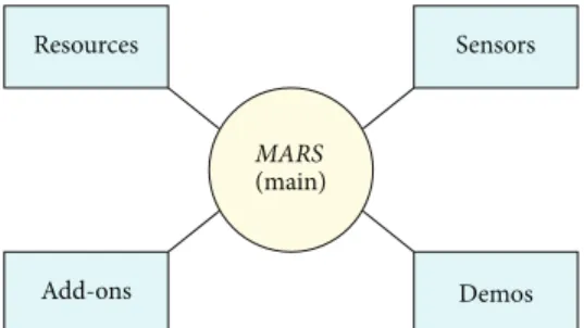
Figure 1: MARS software architecture.

respect to the𝑥-axis. All kinematic equations are discretized

for simulation. Sampling time is set by the user and robots change their status at each time step.

Robots can be equipped with the same controller or with different controllers as well, for example, for experiment involving one leader and many followers. Several types of control strategies can be implemented as follows.

Centralized Control with Full Information. It is assumed that

the complete information about the environment and all robot poses is known by a supervisor controller. At each time step, such a controller is in charge of computing the desired velocities for all agents in the network.

Centralized Control with Partial Information. Unlike the

pre-vious setting, one may assume that the supervisor controller knows only partial information about robot status, like, for instance, position but not orientation.

Distributed Control with Partial Information. Each robot has

to compute its own velocities based on its pose and the poses of some of the other vehicles, for instance, of its neighbors. It may also know partial information about other agents, for example, their position but not their orientation.

Distributed Control with Sensor Information. Agents have to

compute their speed by means of measurements obtained by embedded virtual sensors which provide the only available information.

3. Software Architecture

MARS has been developed in Matlab and consists of a set of

functions which can be divided into five main groups (see Figure 1).

Main File. The file called mars.m represents the main function

of the simulator and it is the function to be launched to run a simulation.

Resource Files. These are functions which can be used by the

main file and/or by users to provide specific functionalities (e.g., check whether collisions occur).

Sensor Files. These functions allow the simulation of virtual

sensors mounted on the robots, like proximity sensors, laser range finders, and so forth.

(3)

Add-Ons Files. MARS allows one to include in the

environ-ment a bunch of features of interests, like the presence of obstacles, Voronoi diagrams, and so forth. Such functionali-ties are implemented through add-ons predefined within the simulator or designed by users.

Demo Files. These files are useful to show demonstrations of

the simulator functionalities. They can be used as a starting point to develop new experiments.

Hereafter, the main file (mars.m) is described in detail. This is the file the user has to run to start the simulation. It consists of a Matlab function whose syntax is defined as follows:

[out data] = mars (exp file, stop time, speed, options)

(i) exp file is the name of the function containing the experiment to be simulated, which has to be defined by the user. Demo files can be used as well. This is a mandatory input parameter.

(ii) stop time specifies the time duration of the experi-ment in seconds.

(iii) speed denotes the playback speed of the simulation.

speed = 1 (default) means that the simulation runs at

actual time; that is, the duration of the simulation is the same as that of the real experiment. Greater values can be used to increase the simulation speed, while lower values can be used to decrease it. Special values are speed = 0 which means “manual mode”; that is, simulation proceeds at each key pressed, and speed = “max” which runs the simulation at the maximum speed allowed by the available computational power. (iv) options is a structure defining options to be used in

the simulation. All the fields of the experiment status structure (Exp status) can be set, see Table 1.

(v) out data is a structure containing all the experi-ment data including robot poses, sensor outputs, and workspace features for each time step. This dataset is useful to perform offline analysis of the experiment. All the data involving a simulation are internally stored in the experiment status structure called Exp status. Such a structure contains data which remain constant over time, like the mechanical characteristics of the robots, as well as dynamical variables like robot poses. The main fields of

Exp status are reported in Table 1.

The body of mars.m can be divided into 3 sections.

Parameter Definition. In this section, default values are

assigned to parameters governing the experiment, like, for instance, the default sampling time, the workspace geometry, and the vehicles characteristics. Such parameters can be changed by the user both from the command line (setting the

options parameter in the MARS call, as described above) and

from the user-defined function of the experiment (exp file).

Initialization. During this phase, the experiment file exp file

is checked and relevant information is set, like the number of

for T=0:sampling time:stop time - update animation

- run addons loop functions - generate sensor measurements - synchronize simulation - execute control function - check motor saturation

- check if robot inside the workspace - check if the experiment is over - update robot pose

end

Algorithm 1: Sketch of the routines inside the main loop.

robots used, their initial conditions, the animation parame-ters, and the used add-ons. Moreover, experiment parameters are overwritten if specified.

Main Loop. This section is in charge of simulating the

exper-iment and can be seen as the core of the project. A sketch of the main commands executed inside the loop is shown in Algorithm 1. The loop is repeated every sampling time and it is synchronized on the basis of the playback speed. At each time step, robot dynamics, sensor measurements, and add-ons routines are computed and the animation is updated. Additional computations concern collision detection and the storage of data in the output structure out data.

On the user side, the only thing to do is to generate the experiment control file. Let us assume that exp file.m is the name of the user-defined file defining the experiment controller. This file has to adhere to the following syntax:

[Command, Exp status] = exp file (Exp status, Init flag)

(i) Exp status denotes the experiment status structure. The main structures fields are listed in Table 1. (ii) Init flag is a boolean variable establishing whether the

simulator is in the initialization or in the simulation phase.

(iii) Command is a matrix containing the desired input speeds of all the robots at the current time step. The task of the user can be summarized as follows. By exploiting the data contained in Exp status, design a control law for each robot which returns a desired robot speed. For holonomic robots, exp file has to generate the

velocitiesV_𝑥,𝑖(𝑡), V_𝑦,𝑖(𝑡) along the two cartesian axes, while for

nonholonomic robots it has to return the linear and angular

velocities,V_𝑖(𝑡) and 𝜔_𝑖(𝑡).

Therefore, to sum up, the user has just to freely write the code of the desired control law generating the desired veloc-ities and finally pack them up within the matrix Command with the following structure:

(i) Holonomic robots:𝐶𝑜𝑚𝑚𝑎𝑛𝑑 = [VV𝑥,1𝑦,1VV𝑥,2𝑦,2⋅⋅⋅ V⋅⋅⋅ V𝑥,𝑛𝑦,𝑛]

(ii) Nonholonomic robots:𝐶𝑜𝑚𝑚𝑎𝑛𝑑 = [V1 V2 ⋅⋅⋅ V𝑛

(4)

Table 1: Description of main Exp status fields.

Field name Description

Robots Number of robots used (default = 1)

Pose Robots pose [𝑥 (meters); 𝑦 (meters); angle (radians)]

Initial pose Initial pose of robots

Sampling time Sampling time (seconds)

Iteration Actual iteration of the main simulation loop

Time Elapsed experiment time (seconds)

Stop time Max duration of the experiment (seconds)

Workspace Vertexes defining the polygonal workspace in clockwise order

Bounds Bounds of the outer box of the workspace (meters) [min𝑥, max 𝑥, min 𝑦, max 𝑦] Non-holonomic True if robots have nonholonomic drive; false for holonomic drive (default = true)

Command delay Transmission delay (seconds)

Geometric center Coordinates of the geometric center of the robot

Exp over True if the experiment is over

Exp over msg Message describing why the experiment is over

Filename Name of the controller file

Version Simulator version

Addons List of add-ons to be used

Addons suffix List of suffixes to be used in add-on’s filename

Robot Robot mechanical characteristics

Robot.Max linear speed Maximum linear speed (m/s) Robot.Wheels semiaxis length Semiaxis length (m)

Robot.Diameter Diameter of robot chassis (m)

Robot.Distance center barycenter Distance from the geometric center of the robot to the center of rotation

Animation Animation structure

Animation.Title Title of the simulation (default = “[Simulation]”) Animation.Grid Enable/disable grid (default = true)

Animation.Show initial pose Show/hide initial pose of robots (default = true)

Animation.Show real shape If true, the actual robot shape is shown; otherwise, a pointwise robot is depicted (default = true) Animation.Wake Enable/disable robots’ wake (default = true)

Animation.Wake style If wake is enabled, use the defined style; styles are the same as in the Matlab function plot (default = “-”)

Animation.Playback speed Simulation playback speed in seconds (default = 1) Animation.Enable Enable the animation (default = true)

Animation.Base colors Base colors to be used in the animation; they will be repeated if needed

Animation.Colors Robot colors to be used in the animation; they are computed repeating the base colors if needed

History Historical data structure

History.Time Simulation time

History.Pose Robot pose

History.Command Robot command

History.Command time Time when the command is received

where 𝑛 is the number of robots, specified by Exp status.

Robots.

4. Session Description

In this section, an illustrative session example is reported along with the Matlab code needed to implement it. As

described in the previous section, the user has to provide a control file (Example random.m in this session example) which generates the desired robot velocities at each time sample.

The aim of this experiment is to drive two robots in a

squared environment of10 × 10 meters. Robots are equipped

(5)

1 function [Command,Exp]=Example random(Exp,Initialization) 2 3 if Initialization 4 Exp.Robots=2; 5 Exp.Workspace=[0 0; 0 10; 10 10; 10 0]; 6 Exp.Animation.Title='[Random movements]'; 7 Exp.Initial pose=[1 3 0; 9 7 pi]';

8 Exp.Animation.Grid=0; 9 10 Exp.Addons={'Map'}; 11 V(1).Vertex=[ 5 2; 4 3; 6 4; 5 3]; 12 V(2).Vertex=[ 4 5; 3 7; 2 8; 1 6; 2 5]; 13 V(3).Vertex=[ 6 6; 7 7; 8 6]; 14 V(4).Vertex=[10 0; 10 10]; 15 V(5).Vertex=[ 0 0; 0 10]; 16 V(6).Vertex=[ 0 10; 10 10]; 17 V(7).Vertex=[ 0 0; 10 0]; 18 Exp.Map.Obstacle=V; 19 20 for i=1:Exp.Robots

21 Exp=Add sensor(Exp,i,{'ProximitySensor'}); 22 Exp.Agent(i).Sensor(1).Range=0.3; 23 end 24 25 Command=[]; return 26 end 27 28 for i=1:Exp.Robots 29 if Exp.Agent(i).Sensor(1).Presence 30 Command(:,i)=[-0.2; 0];

31 elseif (Exp.Iteration>1)&&(Exp.History.Command(Exp.Iteration-1,1,i))<0, 32 Command(:,i)=[0; pi/2+rand(1)*pi];

33 else

34 Command(:,i)=[0.2; 0];

35 end

36 end

Algorithm 2: Matlab code implementing the illustrative example of Section 4.

true if an obstacle or a robot is closer than a prescribed range

(0.3 m in this example). The linear speed of both robots is set as 0.2 m/s, while the angular speed is set as 0 if no obstacle is detected. Whenever a robot detects an obstacle or the other robot, it goes backward for one time step and then it rotates with a random angle. The sampling time is set as 1 second.

The overall Matlab code implementing the required task is reported in Algorithm 2, while the simulation output after 1000 s is depicted in Figure 2. The simulation is run by the following command: out data = mars(“Example random”,

1000, “max”).

Initialization (Lines 3–26)

Lines 4–8. Several parameters are defined, includ-ing the number of robots used in the experiment, the workspace shape and size, and the initial poses of the vehicles.

Line 10.The add-on Map is loaded. It generates the

new substructure Exp.Map containing all the infor-mation about the map.

Lines 11–18. Obstacles are defined through their vertices. In lines 14–18, “fictitious” obstacles are defined at the workspace boundary to prevent robots from exiting the environment.

Lines 20–23. In line 21, each robot is equipped with a proximity sensor, while in line 22 it is set to detect obstacles around a circle with radius 0.3 m.

Line 25.It includes a mandatory code at the end of

the initialization section.

Body (Lines 28–36)

Lines 29-30. For each robot, line 29 checks whether the sensor detects the presence of an obstacle or a robot inside its field of view. If a presence is found, the robot is asked to go backward with a linear velocity of 0.2 m/s and an angular speed of 0. Otherwise, condition in 31 is evaluated.

Lines 31–35. Condition in line 31 checks whether the linear speed at the previous time step was negative

(6)

0 1 2 3 4 5 6 7 8 9 10 0 1 2 3 4 5 6 7 8 9 10 X (m) Y (m)

T = 1000.0 sec (max speed) (random movements)

Figure 2: Illustrative example of two robots moving randomly in an environment with obstacles.

(and the iteration number is greater than one to prevent errors). If so, the robot stops and turns with

a random angle between𝜋/2 and 3/2𝜋; otherwise, it

proceeds straight.

5. Teaching Experiences

Two types of educational experiences based on MARS have been assessed in the recent past, involving secondary school and bachelor students, respectively.

5.1. Secondary School Student Experiences. This experience

regards 31 secondary school students who came to the university for a short stage, with the aim of stimulating their creativity and passion towards engineering topics. This activity dealt with a pursuer-evader game with one pursuer and one evader. The aim of the pursuer is to “catch” the evader, that is, to collide with it, while the evader should avoid collision. After a given time, if no collision occurs, the evader wins; otherwise, it loses. Students were asked to gather in small groups and design a control law for the evader agent. They knew the pursuer strategy which consists in going towards the evader at each time step. The evader speed was initially set as twice the pursuer speed. Then, the latter was gradually increased to make the game more challenging.

Several different control algorithms were devised by various groups. An effective solution relates to a strategy which alternatively drives the evader to one of the four corners of the rectangular workspace depending on the pursuer position (Figure 3). Such an algorithm allows the evader to escape from the pursuer when the speed ratio between the pursuer and the evader is up to 0.9. Of course, different initial positions led to different results. Moreover, it

0 0.5 1.5 2.5 3.5 4.5 5 0 0.5 1.5 2.5 3.5 4.5 5 1 1 2 2 3 3 4 4 X (m) Y (m)

T = 500.0 sec (max speed) (NaifPEG)

Figure 3: Pursuer-evader game, evader controller implemented by secondary school students. Robot poses after 500 seconds. Pursuer: blue; evader: red.

was shown to students that a slower pursuer is still able to capture the evader when using more clever strategies.

5.2. Undergraduate Student Experiences. Another

educa-tional activity which makes use of MARS is related to specific projects carried out by bachelor students, who were asked to implement control algorithms available in the literature, performing a number of different tasks. Only one student is usually involved in a given assignment. Some of these experiences are reported in the next session, concerning tasks such as coverage, pursuer-evader games, cyclic pursuit, collective circular motion, and path planning.

6. Session Examples

In this section, five simulation experiments are described to illustrate the features and capabilities of the proposed simulator. All the controllers have been implemented by bachelor students as a part of their final exam project. In all the experiences, robots are assumed to be nonholonomic drive vehicles.

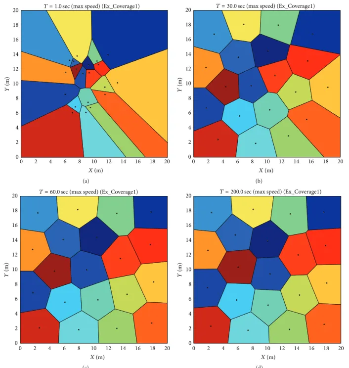
6.1. Coverage. Coverage tasks for multiagent systems consist

in arranging them to optimally cover a given environment, that is, to place them in suitable positions in order to min-imize a given cost function. A convex environment is assumed and a density function representing the importance of different areas is given.

An undergraduate student was asked to implement the distributed control strategy described in [18]. Such a control law is an extension of the Lloyd algorithm [19] and it is based on the central Voronoi partitions of the environment [20].

(7)

0 2 4 6 8 10 12 14 16 18 20 0 2 4 6 8 10 12 14 16 18 20 X (m) Y (m)

T = 1.0 sec (max speed) (Ex_Coverage1)

(a) 0 2 4 6 8 10 12 14 16 18 20 0 2 4 6 8 10 12 14 16 18 20 X (m) Y (m)

(b) 0 2 4 6 8 10 12 14 16 18 20 0 2 4 6 8 10 12 14 16 18 20 Y (m) X (m)

(c) 0 2 4 6 8 10 12 14 16 18 20 0 2 4 6 8 10 12 14 16 18 20 Y (m) X (m)

(d)

Figure 4: Coverage Example1. Voronoi cells assigned to each robot for different times. (a) 𝑡 = 1 s. (b) 𝑡 = 30 s. (c) 𝑡 = 60 s. (d) 𝑡 = 200 s.

Therefore, Voronoi cells and their corresponding centroids were computed by means of the Voronoi add-on in MARS.

As a first example, an experiment involving 20 robots, uniform density, and square workspace has been performed,

whose simulation results are reported in Figure 4. After𝑡 = 60

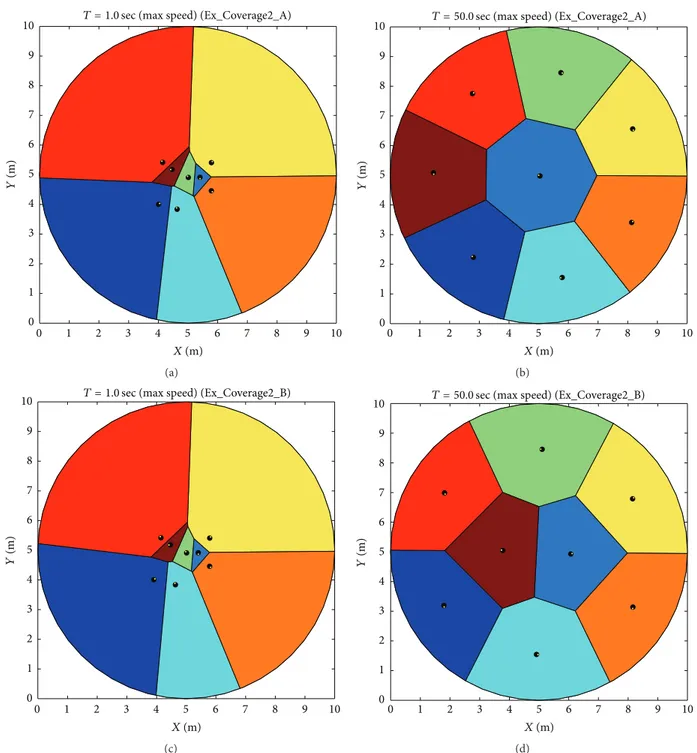
seconds, robots almost reached their steady state position. Since the implemented algorithm does not guarantee attaining the global minimum of the performance cost, it may happen that slightly different initial positions give rise to quite different final ones. Such a behaviour is shown in Figure 5 for 8 robots moving in a circular environment, using

the same control strategy described above. In particular, the initial positions of the two experiments differ only for the position of one robot for 0.1 m. This experience helps students to get acquainted with the key concepts like nonconvex optimization and sensitivity to initial conditions.

6.2. Pursuer-Evader Game. A pursuer-evader game with one

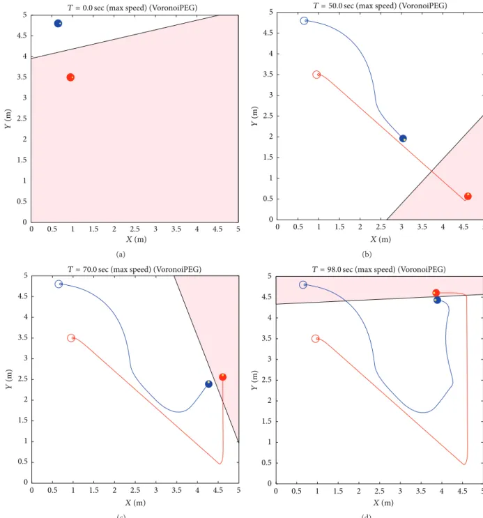
pursuer and one evader is considered. The aim is to imple-ment the pursuer strategy reported in [21]. Let us name this control law VoronoiPEG. Such a strategy is based on the Voronoi partition of the workspace and aims at increasing

(8)

0 1 2 3 4 5 6 7 8 9 10 0 1 2 3 4 5 6 7 8 9 10 X (m) Y (m)

T = 1.0 sec (max speed) (Ex_Coverage2_A)

(a) 0 1 2 3 4 5 6 7 8 9 10 1 2 3 4 5 6 7 8 9 10 X (m) Y (m) 0

T = 50.0 sec (max speed) (Ex_Coverage2_A)

(b) 0 1 2 3 4 5 6 7 8 9 10 0 1 2 3 4 5 6 7 8 9 10 X (m) Y (m)

T = 1.0 sec (max speed) (Ex_Coverage2_B)

(c) 0 1 2 3 4 5 6 7 8 9 10 0 1 2 3 4 5 6 7 8 9 10 X (m) Y (m)

T = 50.0 sec (max speed) (Ex_Coverage2_B)

(d)

Figure 5: Coverage Example2. Voronoi cells assigned to each robot for different times. (a) Initial configuration experiment A (𝑡 = 1 s). (b) Final configuration experiment A (𝑡 = 50 s). (c) Initial configuration experiment B (𝑡 = 1 s). (d) Final configuration experiment B (𝑡 = 50 s).

the area of the Voronoi cell associated with the pursuer at each time instant. In [21], it is proved that the area of the Voronoi cell associated with the pursuer is increasing at each time step under any admissible evader strategy. Eventually, the evader cell reduces to zero with the consequent capture by the pursuer.

In the reported example, it is assumed that the speed of the pursuer is set as 80% of the speed of the evader. The evader will move alternatively to four points near the corners of the

workspace, depending on the current position of the pursuer. The initial condition is shown in Figure 6(a). Empty and filled circles denote the initial and final poses of the robots, respectively. Robot paths are denoted by solid lines, while the light red area denotes the Voronoi cell associated with the evader (red circle). Figures 6(b) and 6(c) show the path of the two vehicles at different times. In Figure 6(d), the final configuration of the robots is displayed, showing the capture of the evader by the pursuer.

(9)

0 0.5 1 1.5 2 2.5 3 3.5 4 4.5 5 0 0.5 1 1.5 2 2.5 3 3.5 4 4.5 5 X (m) Y (m)

T = 0.0 sec (max speed) (VoronoiPEG)

(a) 0 0.5 1 1.5 2 2.5 3 3.5 4 4.5 5 0 0.5 1 1.5 2 2.5 3 3.5 4 4.5 5 X (m) Y (m)

(b) 0 0.5 1 1.5 2 2.5 3 3.5 4 4.5 5 0 0.5 1 1.5 2 2.5 3 3.5 4 4.5 5 X (m) Y (m)

(c) 0 0.5 1 1.5 2 2.5 3 3.5 4 4.5 5 0 0.5 1 1.5 2 2.5 3 3.5 4 4.5 5 X (m) Y (m)

(d)

Figure 6: Pursuer-evader game example. Pose of each robot for different times. (a) Initial robot poses. (b)𝑡 = 50 s. (c) 𝑡 = 70 s. (d) Final robot poses (𝑡 = 98 s). Pursuer: blue; evader: red; evader Voronoi cell: light red.

6.3. Cyclic Pursuit. Cyclic pursuit is a well studied problem

in formation control. In this experiment, six vehicles are assumed to be distinguishable and labeled from 1 to 6. Each

agent has to pursue the next one; that is, robot 𝑖 has to

follow robot 𝑖 + 1 (modulo 6). It is assumed that each

robot is equipped with an ideal sensor which allows it to detect the position and orientation of the robot it has to follow. The aim is to design a control algorithm driving each robot, stabilizing the platoon to regular formations. In this experiment, the decentralized control law described in [22]

has been implemented, with the aim of driving vehicles around a circular trajectory. Each robot independently com-putes its linear and angular speed, proportional to the distance and the orientation of its preceding neighbor. With a suitable choice of the controller gains, a circular forma-tion with equally spaced vehicles is eventually achieved, as depicted in Figure 7. This experience helps the student to understand the role of the controller parameters and to analyze how the formation scales with the number of robots in the team.

(10)

0 1 2 3 4 5 6 7 0 1 2 3 4 5 6 7 X (m) X (m) Y (m)

T = 0.0 sec (max speed) (cyclic pursuit)

(a) Y (m) 0 1 2 3 4 5 6 7 0 1 2 3 4 5 6 7 X (m)

(b) 0 1 2 3 4 5 6 7 0 1 2 3 4 5 6 7 X (m) Y (m)

(c) X (m) Y (m) 0 1 2 3 4 5 6 7 0 1 2 3 4 5 6

7 T = 500.0 sec (max speed) (cyclic pursuit)

(d)

Figure 7: Cyclic pursuit example. Pose of each robot for different times. (a) Initial robot poses. (b)𝑡 = 50 s. (c) 𝑡 = 150 s. (d) 𝑡 = 500 s.

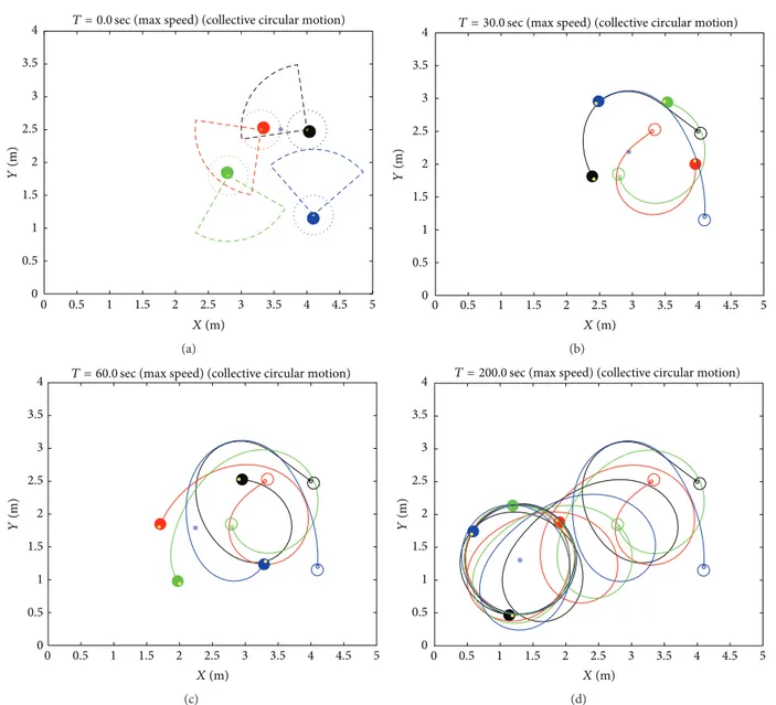
6.4. Collective Circular Motion. This experiment regards

col-lective circular motion of a team of mobile robots [23, 24]. Being different from the previous experiment, here, the platoon is assumed to be composed of indistinguishable vehicles. Each robot is equipped with a range finder sensor able to provide range and bearing measurements of vehicles falling inside a given range and a proximity sensor (e.g., a sonar ring) which returns the presence of the closest vehicle.

The aim of the platoon is to encircle a moving beacon while maintaining a minimum distance among the vehicles and avoiding collisions. The distributed control law devised in [23] has been implemented. An experiment involving four robots pursuing a slow moving beacon is reported in

Figure 8. Here, the beacon moves from[3.6, 2.5]󸀠to[1.3, 1.3]󸀠

following a straight line. The platoon is able to pursue the moving beacon and to stabilize around a circle as soon as

(11)

∗ 0 0.5 1 1.5 2 2.5 3 3.5 4 4.5 5 0 0.5 1 1.5 2 2.5 3 3.5 4 X (m) Y (m)

T = 0.0 sec (max speed) (collective circular motion)

(a) ∗ X (m) Y (m) 0 0.5 1 1.5 2 2.5 3 3.5 4 4.5 5 0 0.5 1 1.5 2 2.5 3 3.5

4 T = 30.0 sec (max speed) (collective circular motion)

(b) 0 0.5 1 1.5 2 2.5 3 3.5 4 4.5 5 0 0.5 1 1.5 2 2.5 3 3.5 4 Y (m) X (m) ∗

(c) Y (m) X (m) 0 0.5 1 1.5 2 2.5 3 3.5 4 4.5 5 0 0.5 1 1.5 2 2.5 3 3.5 4 ∗

(d)

Figure 8: Collective circular example. Pose of each robot for different times. (a) Initial robot poses and sensor field of view. (b)𝑡 = 30 s. (c) 𝑡 = 60 s. (d) 𝑡 = 200 s. Robots are denoted by circles while the beacon is denoted by the asterisk.

the reference stops. Also, in this case, the student can easily challenge the considered technique by changing the sensor range, initial configuration, or the beacon trajectory.

6.5. Path Planning in Complex Environment. To demonstrate

the capabilities of MARS in managing complex environ-ments, in Figure 9, three robots navigating inside the second floor of the authors’ department are shown. The map has been generated in the same way as in the much simpler example in Algorithm 2, after extracting the vertices of each element in the environment from a CAD map. In the experiment, robots are driven by an algorithm based on the artificial potential

field; see [25] for details. They are asked to avoid collisions,

navigate towards a sequence of waypoints, and stop when the last waypoint is reached. Notice that while two robots are able to reach their final destination, the red one gets stuck inside a room. This behaviour is in accordance with a known issue of

controllers based on the artificial potential field method, and students may easily check it. As a possible solution, waypoints should be rearranged or a new waypoint should be added.

7. Conclusions

In this paper, MARS, a Matlab-based simulator for mobile robotics, has been introduced. Such a tool is able to simulate teams of autonomous vehicles performing different tasks. A number of control strategies may be easily implemented, exploiting partial or full information or using data acquired by virtual sensors. In addition, users can design new add-ons and sensors to customize the simulator to specific needs.

The main purpose of this project is educational and it has been used in control systems and robotics courses at the University of Siena. The scope of this facility is not only confined to the educational one, since it can also be used

(12)

0 10 20 30 40 0 10 20 30 40 50 60 70 X (m) Y (m)

T = 700.0 sec (max speed)

(D.I.I.S.M.2nd floor)

Figure 9: Path planning example. Three robots moving in a complex environment through a sequence of waypoints (circles).

for rapid prototyping of new multiagent control algorithms before testing them on real setups.

The MARS project is still under development and several extensions are planned for the near future, like the develop-ment of a graphical interface for defining virtual obstacles, the addition of further virtual sensors, and the simulation of communication protocols between robots. This will lead to a more realistic analysis of complex multiagent systems, such as asynchronous moving sensor networks or teams of heterogeneous mobile robots.

Competing Interests

The authors declare that there are no competing interests regarding the publication of this paper.

References

[1] Cyberbotics Ltd, Webots robot simulator, 2016, https://www .cyberbotics.com/.

[2] M. Freese, S. Singh, F. Ozaki, and N. Matsuhira, “Virtual robot experimentation platform V-REP: a versatile 3D robot simula-tor,” in Simulation, Modeling, and Programming for Autonomous

Robots, N. Ando, S. Balakirsky, T. Hemker, M. Reggiani, and O. von Stryk, Eds., vol. 6472 of Lecture Notes in Computer Science, pp. 51–62, Springer, Berlin, Germany, 2010.

[3] Mobotsoft. MobotSim—Mobile Robot Simulator, 2016, http:// www.mobotsoft.com/?page id=9.

[4] Cogmation Robotics, Virtual Robotics Toolkit, 2016, https:// www.virtualroboticstoolkit.com.

[5] N. Koenig and A. Howard, “Design and use paradigms for Gazebo, an open-source multi-robot simulator,” in Proceedings of the IEEE/RSJ International Conference on Intelligent Robots and Systems (IROS ’04), pp. 2149–2154, October 2004. [6] A. Koestler and T. Br¨aunl, “Mobile robot simulation with

realis-tic error models,” in Proceedings of the International Conference on Autonomous Robots and Agents (ICARA ’04), vol. 1, pp. 46– 51, 2004.

[7] S. Carpin, M. Lewis, J. Wang, S. Balakirsky, and C. Scrapper, “USARSim: a robot simulator for research and education,” in Proceedings of the IEEE International Conference on Robotics and Automation (ICRA ’07), pp. 1400–1405, Rome, Italy, April 2007. [8] R. Vaughan, “Massively multi-robot simulation in stage,” Swarm

Intelligence, vol. 2, no. 2–4, pp. 189–208, 2008.

[9] J. L. Guzm´an, M. Berenguel, F. Rodr´ıguez, and S. Dormido, “An interactive tool for mobile robot motion planning,” Robotics and Autonomous Systems, vol. 56, no. 5, pp. 396–409, 2008. [10] G. Echeverria, N. Lassabe, A. Degroote, and S. Lemaignan,

“Modular open robots simulation engine: MORSE,” in Pro-ceedings of the IEEE International Conference on Robotics and Automation (ICRA ’11), pp. 46–51, IEEE, Shanghai, China, May 2011.

[11] The LEGO Group, “The Lego Mindstorms home page,” 2016, http://mindstorms.com.

[12] M. Casini, A. Garulli, A. Giannitrapani, and A. Vicino, “A matlab-based remote lab for multi-robot experiments,” in Pro-ceedings of the 8th IFAC Symposium on Advances in Control Education (ACE ’09), pp. 162–167, Kumamoto, Japan, October 2009.

[13] M. Casini, A. Garulli, A. Giannitrapani, and A. Vicino, “A LEGO mindstorms multirobot setup in the automatic control telelab,” in Proceedings of the 18th IFAC World Congress, pp. 9812–9817, Milan, Italy, 2011.

[14] M. Casini, A. Garulli, A. Giannitrapani, and A. Vicino, “A remote lab for experiments with a team of mobile robots,” Sensors, vol. 14, no. 9, pp. 16486–16507, 2014.

[15] M. Casini, A. Garulli, A. Giannitrapani, and A. Vicino, “A remote lab for multi-robot experiments with virtual obstacles,” in Proceedings of the 9th IFAC Symposium on Advances in Control Education (ACE ’12), pp. 354–359, Nizhny Novgorod, Russia, June 2012.

[16] M. Casini, A. Garulli, A. Giannitrapani, and A. Vicino, “Remote pursuer-evader experiments with mobile robots in the auto-matic control telelab,” in Proceedings of the 10th IFAC Sympo-sium on Advances in Control Education (ACE ’13), pp. 66–71, Sheffield, UK, August 2013.

[17] M. Casini and A. Garulli, “MARS: a Matlab simulator for mobile robotics experiments,” in Proceedings of the 11th IFAC Symposium on Advances in Control Education, pp. 69–74, Bratislava, Slovakia, June 2016.

[18] J. Cort´es, S. Mart´ınez, T. Karatas¸, and F. Bullo, “Coverage control for mobile sensing networks,” IEEE Transactions on Robotics and Automation, vol. 20, no. 2, pp. 243–255, 2004.

(13)

[19] S. P. Lloyd, “Least squares quantization in PCM,” IEEE Transac-tions on Information Theory, vol. 28, no. 2, pp. 129–137, 1982. [20] Q. Du, V. Faber, and M. Gunzburger, “Centroidal Voronoi

tes-sellations: applications and algorithms,” SIAM Review, vol. 41, no. 4, pp. 637–676, 1999.

[21] H. Huang, W. Zhang, J. Ding, D. M. Stipanovi´c, and C. J. Tomlin, “Guaranteed decentralized pursuit-evasion in the plane with multiple pursuers,” in Proceedings of the 50th IEEE Conference on Decision and Control and European Control Conference (CDC-ECC ’11), pp. 4835–4840, Orlando, Fla, USA, December 2011.

[22] J. A. Marshall, M. E. Broucke, and B. A. Francis, “Pursuit for-mations of unicycles,” Automatica, vol. 42, no. 1, pp. 3–12, 2006. [23] N. Ceccarelli, M. Di Marco, A. Garulli, and A. Giannitrapani, “Collective circular motion of multi-vehicle systems,” Automat-ica, vol. 44, no. 12, pp. 3025–3035, 2008.

[24] D. Benedettelli, M. Casini, A. Garulli, A. Giannitrapani, and A. Vicino, “A LEGO Mindstorms experimental setup for multi-agent systems,” in Proceedings of the IEEE International Con-ference on Control Applications (CCA ’09), pp. 1230–1235, Saint Petersburg, Russia, July 2009.

[25] O. Khatib, “Real-time obstacle avoidance for manipulators and mobile robots,” The International Journal of Robotics Research, vol. 5, no. 1, pp. 90–98, 1986.

(14)

International Journal of

Aerospace

Engineering

Hindawi Publishing Corporation

http://www.hindawi.com Volume 2014

Robotics

Journal of

http://www.hindawi.com Volume 2014 Active and Passive Electronic Components

Control Science and Engineering

Journal of

Hindawi Publishing Corporation

http://www.hindawi.com Volume 2014

Machinery

http://www.hindawi.com Volume 2014 Hindawi Publishing Corporation

http://www.hindawi.com

Journal of

Engineering

Volume 2014

Submit your manuscripts at

http://www.hindawi.com

VLSI Design

Hindawi Publishing Corporation

http://www.hindawi.com Volume 2014

Shock and Vibration

Civil Engineering

Advances in

Acoustics and VibrationAdvances in

Electrical and Computer Engineering

Journal of

Advances in OptoElectronics

Hindawi Publishing Corporation

http://www.hindawi.com Volume 2014

The Scientific

World Journal

Sensors

Journal of Hindawi Publishing Corporation

Modelling & Simulation in Engineering

http://www.hindawi.com Volume 2014 Chemical Engineering

International Journal of Antennas and Propagation International Journal of

Navigation and Observation International Journal of

MARS: An Educational Environment for Multiagent Robot Simulations

Research Article