Nonlinear analysis of structures on elastic half-space by a FE-BIE approach

Università degli Studi di Ferrara

DOTTORATO DI RICERCA IN

"SCIENZE DELL’INGEGNERIA"

COORDINATORE Prof. Stefano Trillo

Nonlinear analysis of structures

on elastic half-space

by a FE-BIE approach

Settore Scientifico Disciplinare ICAR/09

Dottorando Tutore

Dott. Baraldi Daniele Prof. Tullini Nerio

Nonlinear analysis of structures on elastic half-space by a FE-BIE

approach

PhD Thesis by Daniele Baraldi

Supervisor

Prof. Nerio Tullini

March 2013

Università degli Studi di Ferrara

Dottorato di Ricerca in Scienze dell’Ingegneria Ingegneria Civile − Tecnica delle Costruzioni XXV ciclo

Examiners:

Prof. Antonio Tralli, Università di Ferrara Prof. Fabio Conti, Università dell’Insubria Prof. Giorgio Novati, Politecnico di Milano

Contents

Introdutcion ...1

1 Stability of Euler-Bernoulli beams and frames resting on elastic

half-plane...5

1.1 Introduction ... 5

1.2 Basic relationships... 7

1.3 Discrete model... 9

1.4 Comparison of the present model with a traditional FE model ... 12

1.4.1 Convergence test for a beam with free ends ... 13

1.5 Buckling analysis of beams resting on elastic half-plane ... 17

1.5.1 Analytic solution for the buckling of a beam of infinite length resting on an elastic half-plane... 17

1.5.2 Beam of finite length with sliding ends ... 20

1.5.2.1 Modal shapes... 23

1.5.2.2 Beam with sliding ends on Winkler-type half-space ... 26

1.5.3 Beam of finite length with pinned ends ... 30

1.5.3.1 Modal shapes... 33

1.5.3.2 Bosakov’s solution (1994) ... 37

1.5.3.3 Gallagher’s solution (1974)... 38

1.5.3.4 Beam with pinned ends on Winkler-type half-space ... 41

1.5.4 Beam of finite length with free ends ... 44

1.5.4.1 Modal shapes... 46

1.5.4.2 Beam with free ends on Winkler-type half-space... 48

1.5.5 Beam of infinite length with various end restraints ... 51

1.5.6 Buckling of a beam with a weakened section at midpoint... 53

1.6 Analysis of a compressed beam on half-plane loaded at midpoint... 58

1.6.1 Incremental analysis of a compressed beam on half-plane loaded at midpoint... 62

1.7 Rectangular pipe resting on elastic half-plane ... 64

1.7.1 Buckling of rectangular pipes with free and pinned foundation beam ends ... 65

1.7.1.1 Buckling of rectangular pipes on half-plane modelled with traditional FEs... 70

2 Stability of Timoshenko beams resting on elastic half-plane...77

2.1 Introduction ... 77

2.2 Basic relationships... 79

2.3 Discrete model... 81

2.4 Comparison of the present model with a classical FE model ... 84

2.4.1 Convergence test for a beam with free ends ... 84

2.5 Buckling analysis of beams with different end restraints ... 87

2.5.1 Beam of finite length with pinned ends ... 87

2.5.1.1 Modal shapes... 91

2.5.1.2 Two-dimensional FE model results ... 94

2.5.1.3 Buckling of a beam with pinned ends on Winkler half-space ... 97

2.5.2 Beam of finite length with free ends ... 100

2.5.2.1 Modal shapes... 103

2.5.2.2 Two-dimensional FE model results ... 106

2.5.2.3 Buckling of a beam with free ends on Winkler half-space... 109

2.5.2.4 First critical load determined with different beam models ... 111

2.6 Coupling of 2D plane elements and boundary integral equations ... 112

2.6.1 Basic relationships... 112

2.6.2 Discrete model... 114

2.6.3 Static analysis of a layer resting on an elastic half-plane ... 116

2.6.4 Buckling analysis of 2D beams with free ends on half-plane... 119

3 Analysis of slender beams and frames resting on elastic

half-plane including material nonlinearity...125

3.1 Introduction ... 125

3.2 Semi-rigid analysis for a beam-column element... 127

3.2.1 Monforton-Wu-Xu model for a beam with semi-rigid ends... 127

3.2.2 Shakourzadeh model for a beam with semi-rigid ends... 129

3.3 Plasticity model for a beam-column element... 133

3.4 Analysis of beams on elastic half-plane including material nonlinearity... 136

3.4.1 Beam with plastic hinges on elastic half-plane... 136

3.4.2 Incremental analysis of beams on half-plane including material nonlinearity... 137

3.4.3 Incremental analysis of beams on half-plane including material and geometric nonlinearity... 144

3.5 Incremental analysis of frames on half-plane including material nonlinearity

... 146

3.5.1 Description and design of the structure... 146

3.5.2 Description of the discrete model ... 150

3.5.3 Numerical examples: pipe loaded by increasing service loads... 152

3.5.3.1 Example 1: pipe loaded by a distributed force along the upper beam.. 152

3.5.3.2 Example 2: pipe loaded by self-weight and service load along the upper beam ... 154

3.5.3.3 Example 3: pipe loaded by dead loads and increasing service loads.... 156

4 Static and buckling analysis of beams resting on 3D elastic

half-space...161

4.1 Introduction ... 161

4.2 Half space model... 163

4.3 Galerkin boundary element method ... 164

4.3.1 Surface discretization ... 165

4.3.2 Rigid rectangular punch on elastic half-space ... 168

4.3.3 Uniform pressure... 176

4.4 Beam model... 183

4.4.1 Analytical formulation ... 183

4.4.1.1 Kinematical model ... 184

4.4.1.2 Constitutive laws ... 187

4.4.1.3 Formulation of the linearized stability problem... 188

4.4.2 Beam discrete model ... 191

4.4.2.1 Interpolating shape functions ... 192

4.5 Beam on 3D half space... 194

4.5.1 Variational formulation ... 195

4.5.2 Discrete model... 197

4.6 Static analysis of beams on 3D elastic half-space... 201

4.6.1 Foundation beam loaded by a concentrated force at midpoint ... 201

4.6.2 Foundation beam loaded by a uniform force distribution... 210

4.6.3 Foundation beam loaded by a concentrated moment at midpoint ... 213

4.7 Buckling analysis of beams on 3D elastic half-space ... 217

4.7.1 Beam with sliding ends ... 217

4.7.3 Beam with free ends... 223

4.7.4 Critical loads of a beam on stiff half-space varying L/b ratio... 226

Conclusions ...229

Appendix A1 – Discrete model for a beam on 2D half-space ... 233

Appendix A2 – Discrete model for a beam on Winkler half-space... 234

Appendix A3 – Discrete model for a layer on 2D half-space... 236

Appendix A4 – Discrete model for a beam with semi-rigid ends (Monforton-Wu-Xu)... 238

Appendix A5 – Discrete model for a beam on 3D half-space ... 240

Introduction

The analysis of the interaction between deformable bodies represent a problem with both a mathematical and an engineering interest. In the engineering field, such interaction problems include, for example, the study of structural shallow foundations, floating structures, laminated or composite materials, sandwich panels, indentation problems. In the civil engineering field, the analysis of the interaction between structural foundations and the supporting soil is important to both structural and geotechnical engineering. Results of soil-structure interaction (SSI) analyses provide information which may be used in structural design of the foundation or of the entire structure, or in the analysis of stresses and deformation within the soil. Even if many studies are devoted to the elastic analysis of the interaction problem, the subject is continually being extended in order to include, for example, material and geometric nonlinearity. The aim of this thesis is to extend an existing numerical approach for studying the SSI problem of beams and frames on elastic half-space, including geometric and material nonlinearities and considering two different types of half-space model. In the civil engineering field, the SSI problem assumes that the soil can be adequately represented by an elastic medium occupying a half-space region. In this thesis, models of half-space response which exhibit linear elastic characteristics are considered. The linear elastic idealization of the supporting medium is often represented by a mathematical model which describes the particular characteristics of the behaviour of the half-space. Some idealizations have been developed during years. The simplest soil or half-space model was defined by Winkler (1867), who assumed that the surface displacement of the half-space at every point is proportional to the pressure applied at the same point and it is independent of pressures and displacements at other surface points. Winkler-type half-space is physically represented by a distributed set of springs under the supported structure and it is often adopted to describe, for example, the behaviour of floating structures, railroad tracks and road pavements. Since the deflections in a Winkler model are limited to the loaded region, this reduce the applicability of the model, which turn out to be quite different than the real behaviour of a half-space characterized by transmissibility of applied forces such as the soil medium, the core of a sandwich panel or the elastic support of a thin film. In these cases, an elastic continuum model may be defined. The initial

studies in this context were done by Boussinesq (1885), who analyzed the problem of a semi-infinite homogeneous and isotropic linear elastic solid subject to a concentrated force acting normal to the its surface. A similar case is given by the plane problem of a concentrated normal line load applied to the surface of the half-space, which was studied for the first time by Flamant (Timoshenko and Goodier 1970, Johnson 1985). Moreover, it must be noted that the incapacity of the Winkler model in determining the continuous behaviour of real supports and the complexity of the continuum models caused the development of many other simple half-space response models in the past. Some examples are given by the two-parameter elastic models, which are characterized by two independent elastic constants (Hetenyi 1946, Pasternak 1954, Vlasov and Leonitiev 1966). The interaction between foundations and the supporting soil medium is often analyzed by coupling finite element (FE) and boundary element (BE) methods (Brebbia and Georgiou 1979, Mendonca and Paiva 2003, Gonzalez et al. 2007). FE method is appropriate for structural analysis, whereas BE method is appropriate for studying unbounded domains. Moreover, adopting symmetric Galerkin BEM-FEM coupling procedures (Leung et al. 1995, Springhetti et al. 2007), symmetric coefficient matrices may be obtained for the BE formulations. BE formulation was adopted to study layered soils (Maier and Novati 1987), whereas BEM-FEM coupling may be also adopted for studying fracture mechanics problems (Frangi et al. 2002, Frangi and Novati 2003).

Considering the elastic half-plane or half-space, the BE formulation may be simplified by adopting a simple fundamental solution such as Boussinesq or Flamant solution, respectively. In these cases, the discretization of the contact surface generates a symmetric and positive definite system matrix. The first application of the FE-BE approach was carried out by Cheung and Zinkiewicz (1965) for the static analysis of plates on elastic foundations. The authors discretized the soil reaction with concentrated forces at plate sub-element nodes and obtained the flexibility matrix of the soil by using both Boussinesq and Winkler solutions. In the latter case, the flexibility matrix was purely diagonal. Cheung and Zinkiewicz showed that the stiffness matrix of the soil may be obtained by inverting the flexibility matrix and adding it to the stiffness matrix of the foundation, the total stiffness of the system may be obtained. The same approach was adopted by Cheung and Nag (1968) for the determination of the stiffness matrix of an elastic half-plane (Flamant solution) and half-space (Boussinesq solution). The flexibility matrix of the soil was also used by

Rajapakse and Selvadurai (1986) for studying Mindlin plate elements, whereas Guarracino et al. (1992) studied three-dimensional frames with rigid footings on half-space.

A SSI problem may be studied efficiently adopting a mixed variational formulation, which assumes as independent functions both structure displacements and soil or half-space contact pressures. Kikuci (1980) adopted a mixed variational formulation for studying beams resting on Pasternak soil, whereas Bjelak and Stephan (1983) adopted this formulation for Pasternak soil model and averaging Boussinesq solution. Tullini and Tralli (2010) studied Timoshenko beams on elastic half-plane by coupling beam FEs and boundary integral equation for the half-plane and adopting a mixed variational formulation. The same approach has been adopted by Tullini et al. (2012a) for studying axially loaded thin structures bonded to a homogeneous elastic half-plane.

In the first chapter of this thesis, the simple and efficient numerical model, introduced by Tullini and Tralli (2010), is extended to the buckling analysis of Euler-Bernoulli (E-B) beams on half-plane and to incremental analysis of E-B beams and frames including geometric nonlinearity. The stability of beams on elastic half-plane is important in many engineering fields, such as the design of structural sandwich panels (Allen 1969) and the buckling analysis of thin films in electronic industry (Shield 1994; Volynskii et al. 2000). The stability and the non-linear geometric analysis of frames on elastic half-plane may be very important for the design of subways or box-culverts. Moreover, the coupling of foundation FEs with a structure described by traditional beam elements, including geometric nonlinearity, represents a promising aspect of this work. In the second chapter, buckling analysis of beams on half-plane is applied to the Timoshenko beam model, which is well suited to study structural foundations with low slenderness. The results showed in first and second chapter have recently been published (Tullini et al. 2013, Tullini et al. 2012b).

In the third chapter, the analysis of E-B beams and frames on elastic half-plane is carried out including structural material nonlinearity. The non-linear behaviour of beams in bending is considered and for simplicity it is lumped at beam ends and represented by plastic hinges. For this purpose, an efficient model, commonly used to represent semi-rigid connection behaviour (Monforton and Wu 1963, Shakourzadeh et al. 1999), is adopted for representing the non-linear moment-rotation behaviour of beam cross-sections,

following the approach of Hasan et al. (2002) for the pushover analysis of frames. Analysis of foundation beams including material nonlinearity are performed by defining a-priori the position of potential plastic hinges. Then, a box-culvert designed to grant the flow of a river under a railway line is studied and an incremental analysis is performed.

Finally, in the fourth chapter, the three-dimensional (3D) half-space model is considered and the flexibility matrix of the soil represented by Boussinesq solution is determined. The Galerkin boundary element method is firstly applied for solving problems related to rigid indenters on elastic half-space and uniform pressures over rectangular areas. Then, static and buckling analysis of beams on elastic soil is considered and the stiffness matrix of the soil is determined. Foundation beams of 3D frames on elastic soil may be discretized by adopting a beam model based on Timoshenko bending theory and Reissner (1952) torsion theory, following the model described by Minghini et al. (2008). However, for simplicity, foundation beams with rectangular cross-section are considered for static and buckling analysis, whereas surface pressures are discretized by adopting constant shape functions and subdividing the contact surface in both directions. Static analysis results for beams loaded by many load configurations are discussed and buckling analysis results are compared against those obtained with the two-dimensional half-space model.

1 Stability of Euler-Bernoulli beams and frames

resting on elastic half-plane

1.1 Introduction

The stability of Euler-Bernoulli beams and frames resting on substrate or soil is important in many engineering fields and, in the past, this has been the subject of many works. In the civil engineering field, examples of this problem are the lateral buckling of welded railway rails (Kerr 1974, 1978) and the stability of road pavements (Kerr 1984). In this context, the pioneering works of Wieghardt (1922) and Prager (1927) are based on the assumption that the half-space under the beam is modelled as a continuously distributed set of springs (Winkler 1867). In 1937, Biot studied the problem of an infinite beam resting on elastic half-plane loaded by vertical forces. Biot compared beam bending moments with the ones obtained with the Winkler soil model and determined a relation between the Winkler subgrade modulus and the elastic modulus of the half-plane. After Biot, Reissner (1937) was the first to study the stability problem of an infinite beam resting on an elastic half-plane. Identical results were obtained by Murthy (1970, 1973b) who studied the stability of continuously supported beams on elastic half-plane and on a Wieghardt-type half-space. After Reissner results, the interest in this problem grew, motivated by early structural problems of sandwich elements, and Gough et al. (1940) extended Biot and Reissner results to include various conditions of contact between the infinite beam and the elastic half-plane. The study of sandwich elements continued up to recent years (Allen 1969; Ley et al 1999; Davies 2001). Recently, the main interest has been motivated by thin film buckling and by the research driven by the developments in the electronic industry (Shield 1994; Volynskii et al. 2000). The case of buckling without delamination is often called wrinkling.

In Timoshenko and Gere (1961), the buckling of a simply supported Euler-Bernoulli beam on Winkler soil is studied. Other boundary conditions, such as beam with clamped ends and beam with free ends, were studied and compared with the former (Hetenyi 1946). Moreover, the buckling conditions of beam on Winkler half-space with various end restraints were recently resumed by Wang et al. (2005). In the sandwich plates context, Goodier and Hsu (1954) underlined

the presence of nonsinusoidal local buckling modes with large deflections at beam ends.

Assuming the more realistic relationship between foundation pressure and beam displacement defined by Wieghardt, Smith (1969), determined the buckling loads of a beam with pinned ends. Gallagher (1974) was the first to study the buckling of a beam with finite length and pinned ends on elastic half-plane adopting Chebyshev polynomials. The same problem was studied by Bosakov (1994) who applied the Ritz method to solve the stability problem of a simply supported beam.

In this chapter, the critical loads of Euler-Bernoulli beams with finite length resting on an elastic half-plane are evaluated by using the Finite Element-Boundary Integral Equation (FE-BIE) coupling method proposed by Tullini and Tralli (2010), where static analysis is performed. Making use of a parameter that takes into account both beam slenderness and half-plane stiffness, comparisons with analytical solutions and traditional two-dimensional (2D) FEs are given. Then, buckling loads and mode shapes are determined for different beam end restraints. The results are also compared with the corresponding ones obtained with a Winkler space model. Moreover, rectangular frames on elastic half-plane with compressed columns are considered. Buckling loads and mode shapes are determined for two different restraint conditions and varying soil stiffness. In addition, the geometric nonlinear behaviour of the frames is investigated and the load multipliers at limit point are compared with the buckling loads, showing that some pipes stiffer than the soil may exhibit snapthrough instability. Results relative to beam and frame buckling have recently been presented and discussed by Tullini et al. (2013).

1.2 Basic relationships

Fig. 1.1 – Beam on elastic half plane subject to external load p(x) and compressive force P.

An elastic beam of length L, cross-section height h and width b, resting on a semi-infinite linearly elastic substrate in plane state, is referred to a Cartesian coordinate system (0; x, y), where x coincides with both the centroidal axis and the boundary of the half-plane and y is directed downwards. In the following, Eb

and Es indicate the Young moduli of beam and substrate, respectively.

Analogously, Poisson’s ratios of beam and substrate are denoted by b and s,

respectively. Generalized plane stress or plane strain regime is considered; in the latter case, the width b of both beam and half-plane is assumed unitary. The beam is loaded at the ends by a compressive force P as shown in Fig. 1.1. A distributed vertical external load p(x) can also be applied along the beam axis x. In the interface between beam and soil, frictionless and bilateral conditions are assumed. Consequently, a vertical soil reaction r(x) is enforced to both beam and substrate and the vertical displacement v(x) of the beam coincides with that of the half-plane boundary.

The total potential energy b of the Euler-Bernoulli beam resting on the elastic

half plane is given by the strain energy of the beam including second order effects (Bazant and Cedolin 1991), the work of external loads p(x) and half-space reactions r(x). Then, it can be written as:





where prime denotes differentiation with respect to x and Db = E0 bh 3/12 is the

bending stiffness, with E0 = Eb or E0 = Eb/(1b2) for a generalized plane stress

The potential energy of the half-space is given by:



Considering the Clapeyron’s theorem, the strain potential energy of the half-space is equal to half the work of the contact stresses at the beam soil interface (Tullini and Tralli 2010):



Then, the total potential energy of the half-space turns out to be:







where the vertical displacement v(x) is replaced by the boundary integral equation known as Flamant’s solution (Timoshenko and Gere 1961; Johnson 1985), which uses the Green function g(x,xˆ ) corresponding to the solution of the

elastic problem for a homogeneous isotropic half-plane loaded by a point force normal to its boundary:

x x E x x g( , ˆ) 2 ln  ˆ    . (1.5)

The generic elastic modulus of the half space E is equal to Es or Es/(12s) for a

generalized plane stress or plane strain state, respectively.

Constraint equations Ri(v, v') = 0 between displacements or rotations, may be

assigned along the beam axis, especially at beam ends. For example, a beam with pinned ends requires the equation v(L/2)  v(L/2) = 0. These constraint equations can be included in the total potential energy  of the beam-substrate system by means of a penalty approach (Reddy 2006):

2 )] , ( [ 2 ) ( ) , ( ) , (   



where k is the penalty parameter whose value should be large enough to satisfy the constraint equations accurately. For beams with free ends, rigid-body

displacement related to Flamant’s solution can be removed by choosing an arbitrary abscissa x where a null value of v(x) is forced.

1.3 Discrete model

Fig. 1.2 – Beam on elastic half plane subdivided into 8 equal FEs

A simple discretization of the beam can be created by subdividing the beam into FEs of length li (Fig. 1.2), then beam displacements and rotations are discretized

in the usual form as follows

d() = N() qi (1.7)

where  = x/li, d = [v, ]T collects the unknown displacement function, qi = [v1, 1, v2, 2]T = [v1, v’1, v2, v’2]T. Beam shape functions collected in the

matrix N() are the classical Hermitian polynomials and the corresponding derivatives: . 2 3 ); 1 ( ; / ) 1 ( 6 ; 2 3 ; 4 3 ; ) 1 ( ; / ) 1 ( 6 ; 2 3 1 2 24 2 14 23 3 2 13 2 22 2 12 21 3 2 11

































Half-plane pressures are discretized considering a piecewise constant soil reaction inside each element (Tullini and Tralli 2010):

r()= [()]T ri, (1.9)

where ri denotes the vector components of nodal soil reaction and  assembles

constant shape functions. One, two or four subdivisions can be considered inside each element.

Substituting Eqs. 1.8 and 1.9 into variational principal (Eq. 1.6), the total potential energy  written in discrete form takes the expression:

r G r r H q F q q K q r q T T T b T _{b b b} 2 1 2 1 ) , (      (1.10)

where, the penalty function in discrete form is included into the beam stiffness matrix Kb.

Then, the stationarity condition of the total potential energy  written in discrete form provides the following system:

                                 0 F r q G H H K K _b E b b b D PL L D g b b b ~ ~ ~ T 2 3 (1.11)

where the vector q collects nodal displacements, r denotes the vector of constant soil reactions, F is the external load vector, Db/L 3Kb

~ _{is the elastic stiffness} matrix of the beam, P/LKg

~ _{is the geometric (or incremental) matrix. The}

elements of matrices H and G~ , together with the element matrices K~_biand K~_gi,

are reported in the appendix A1.

System in Eq. 1.11 yields the following solution:

q H G r _{ E} ~1 T _{. (1.12)}





where K~_soil is the stiffness matrix of the half-plane

 

and load multiplier , and parameter L are defined as follows;

3 3 2 , b b D L b E L D PL     . (1.15a,b)

According to references (Biot 1937; Vesic 1961; Tullini and Tralli 2010), the parameter L in Eq. 1.15b describes the beam-substrate system. Low values of αL characterise short beams stiffer than the soil, whereas higher values of αL describe more flexible beams, this latter case is suitable to represent long beams resting on stiff soil.

The adopted mixed finite element model is particularly simple and effective, as shown in Tullini and Tralli (2010) for the static case, where the numerical properties of the present FE model are also discussed. As for the determination of critical load Pcr, a homogeneous system associated to Eq. 1.13 must be

considered and the buckling loads are given by the roots cr of the equation

det[K~_b K~ _g K~_soil] = 0, which can be suitably reduced to a standard eigenvalue problem. Making use of Eq. 1.15a and the definition of Euler critical load: 2 2 E cr, L D P _  b _{, (1.16)}

dimensionless buckling loads are defined as Pcr/Pcr,E = cr/2.

In the case of a structure connected to the foundation beam, system (Eq. 1.13) can be partitioned as shown in (Tullini and Tralli 2010), where nodal displacements without or with nodes shared with the foundation beam are selected. Moreover, the element geometric matrix of each beam FE is dealt with as usual.

1.4 Comparison of the present model with a traditional FE model

Taking into account two different αL values, representing a rather stiff beam (αL

= 5) and a flexible beam (αL = 25), a convergence test is done in order to compare the present model with a classical model that uses 2D elastic elements to describe the soil. In both cases, the foundation beam is modelled as Euler-Bernoulli beam subdivided into equal FEs, with a number of elements nel equal

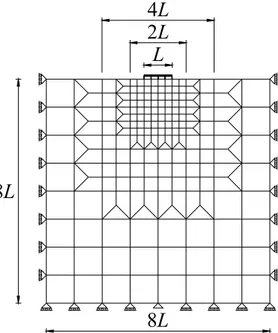
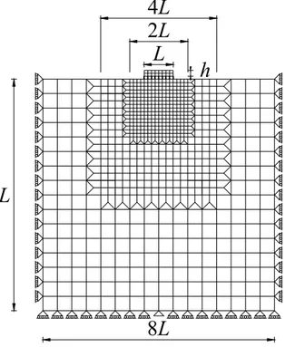
to powers of two up to 512 FEs. Each beam element of the present model includes one soil element, whereas in the 2D model the soil is modelled by a square mesh of quadrilateral elements in plane state. The mesh of the soil has a total width equal to 8L, and zero horizontal and vertical displacements are imposed at vertical and lower boundaries, respectively. Two nested square meshes, which width equal to 4L and 2L, are taken close to the foundation beam, and each quadrilateral element side of the smaller mesh has the same size of the beam element. This type of mesh does obviously require a mix of triangular and quadrilateral elements, in order to avoid hanging nodes and to reduce the total number of degrees of freedom with respect to a mesh of quadrilateral elements only. 8L 8L L 2L 4L

Fig. 1.3 – Mesh adopted for the 2D model with foundation beam subdivided into 4 equal FEs.

In Fig. 1.1.3, the case of the foundation beam subdivided in 4 beam FEs is shown. The frictionless connection between beam and soil nodes is established

by vertical master-slave links. The adopted 2D code uses geometric matrix also for 2D soil FEs.

1.4.1 Convergence test for a beam with free ends

Fig. 1.4a shows the number of equations for the two models, with respect to the number of FEs adopted for the beam. Fig. 1.4b shows the number of equations of the two models with respect to the number of equations of the present model. In both figures the line with crosses is used for the present model and the line with dots regards the 2D model. Adopting axis in logarithmic scale, each set of points lie on a straight line in both figures and the corresponding slope can be calculated through least-squares method. Therefore, the ratio between the number of equations of the two models can be easily determined. Tab. 1.1 collects the number of equations of the 2D model and the present model varying the number of beam elements. The slope of the line with dots in Fig. 1.4b is 2.04, whereas the slope of the line with crosses is obviously equal to 1. The same number can be obtained by determining the ratio between the slopes A of the straight lines in Fig. 1.4a.

04 . 2 95 . 0 / 94 . 1 / PA 2D _{A  } A (1.17) (a) 100 ₁₀1 ₁₀2 ₁₀3 n_elPA_{, n} el2D 100 102 104 106 neq PA , neq 2D 2D model Pres. Analysis 100 102 104 106 neq PA , neq 2D 100 ₁₀1 ₁₀2 ₁₀3 n_eqPA 2D model Pres. Analysis (b)

Fig. 1.4 – Number of equations of 2D model and present model as a function of beam FEs (a) and number of equations of the present model (b).

neq nel 2D model Present Analysis 22 424 10 23 1488 18 24 5536 34 25 21312 66 26 83584 130 27 331008 258 28 1317376 514

Tab. 1.1 – Number of equations for the two models considered, with respect to the number of beam FEs

Therefore, the number of equations of the 2D model 2D eq

n is related to the number

of equations of the present analysis PA eq

n by means of the following relation: 2 ) ( 2 PA 2D eq eq n n  . (1.18) where PA eq

n = 2 nel + 2 as usual, as it can be seen in Tab. 1.1.

The present analysis performed with a beam having 2,048 FEs and one soil reaction under each beam element is used as reference to determine the first three buckling loads REF

cr

P . Figs. 1.5a and b show the relative error Pcr = (PcrFEM

REF cr

P )/ REF

cr

P as a function of nel for L = 5 and 25. Figs. 1.5c and d

show the absolute values of the relative error Pcr in logarithmic scale, in order

to obtain the convergence rates for the critical loads. Lines with dots represent errors for the 2D model, whereas lines with crosses represent errors for the present analysis. It is clear that the first and the second buckling loads obtained with the two models converge with the same rate, which is less than 1

el

n . The

third buckling load converge for both models with a rate larger than the previous one, which is less than 2

el

n . Both methods converge with a rate less than 1

el n for the first two eigenvalues, but CPU time t2D of the 2D model is bigger than 5 (tPA)2.5, where tPA is the CPU time of the present analysis.

(a) L -0.30 -0.15 0.00 0.15 0.30 Pcr 1st 2nd 1st 2nd 3rd -0.30 -0.15 0.00 0.15 0.30 Pcr L 1st, 2nd 1st 2nd 3rd (b) (c) 100 ₁₀1 ₁₀2 ₁₀3 n_el 10-4 10-3 10-2 10-1  Pcr | 10-6 10-5 10-4 10-3 10-2 10-1  Pcr | 100 ₁₀1 ₁₀2 ₁₀3 n_el 1st 2nd 2nd 3rd 1st, 2nd 3rd (d)

Fig. 1.5. Relative errors Pcr for first three buckling loads as a function of nel for L = 5 (a)

and L = 25 (b). Absolute relative errors in bi-logarithmic scale for first three buckling loads L = 5 (c) and L = 25 (d).

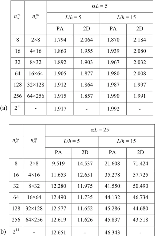
L = 5 PA 2D nel 1 2 3 1 2 3 22 1.688 1.889 4.956 2.267 2.939 4.917 23 1.880 2.131 5.008 2.159 2.630 4.993 24 1.949 2.233 5.019 2.087 2.474 5.017 25 1.977 2.279 5.022 2.046 2.396 5.022 26 1.990 2.300 5.023 2.025 2.356 5.022 27 _{1.996 2.311 5.023 2.014 2.337 5.022} 28 1.999 2.316 5.023 2.008 2.327 5.022 (a) 211 _{2.004 2.318 5.023 - - -} L = 25 PA 2D nel 1 2 3 1 2 3 22 6.776 9.240 29.469 19.454 25.481 46.132 23 23.811 23.849 65.543 60.796 62.307 65.650 24 40.582 40.645 77.512 61.605 61.686 75.049 25 47.595 47.662 78.084 57.851 57.892 77.357 26 50.138 50.201 78.155 55.208 55.257 77.965 27 51.186 51.248 78.165 53.714 53.768 78.118 28 51.663 51.724 78.167 52.926 52.982 78.156 (b) 211 52.059 52.114 78.167 - - -

Tab.2. First three dimensionless critical loads Pcr/Pcr,E corresponding to

the present analysis (PA) or 2D models as a function of nel for L equal to 5 and 25.

Moreover, relative errors are lower than 1% with at least 128 beam FEs for αL = 5 and with at least 256 beam FEs for αL = 25. Thus, the present model can be considered effective for the determination of buckling loads and mode shapes, and a number of 256 equal FEs are adopted for all cases reported in this section.

1.5 Buckling analysis of beams resting on elastic half-plane

In the following, beams with finite length and with different boundary conditions are discussed (sliding-sliding, pinned-pinned and free-free) and for each case, critical loads and modal shapes are determined for increasing values of αL. Moreover, analytic solutions of similar problems such as the ones studied by Reissner (1937), Gallagher (1974) and Bosakov (1994) are present in order to have a comparison for the present analysis.

1.5.1 Analythic solution for the buckling of a beam of infinite length resting on an elastic half-plane

Reissner (1937) studied the stability of a beam of infinite length resting on an elastic half-plane (Fig. 1.6), starting from the differential equation of an Euler-Bernoulli beam on elastic half-plane, including second order effects due to axial load P (Eqs. 1.19a and b).

Fig. 1.6 – Beam of infinite length on elastic half space subject to axial load.

4 2 4 2 ( ) ( ) _{( )} b d v x d v x D P r x dx  dx   (1.19a) ˆ ˆ ˆ ˆ ˆ ˆ ( ) ( , ) ( ) (| |) ( ) v x g x x r x dx g x x r x dx     

_

_

Substituting Eq. 1.19a with Eq. 1.19b and differentiating with respect to x, the following expression is obtained:

x d dx x v d P dx x v d D dx x x g d dx x v d b ˆ ) ˆ ( ) ˆ ( |) ˆ (| ) ( 2 2 4 4           

_

Reissner assumed a solution which satisfies the conditions of vertical displacement and curvature equal to zero for xn = ± nL, with n = 1, 2, 3.. . A

sine-type solution satisfies these conditions:

L x m x

v( ) sin  for m = 1, 2, 3, .. (1.21)

This solution represents a beam which is freely supported at the points xn, then

the original problem of an infinite beam supported by an elastic half plane becomes the problem of an infinite beam resting on elastic half plane supported by an infinite set of equidistant supports. It is worth noting that the buckling modes corresponding to this solution are sinusoidal with constant amplitude. Considering Eq. 1.21, Eq. 1.19 becomes

x d L x m L m P L m D dx x x g d L x m L m b ˆ ˆ sin |) ˆ (| cos 2 4                              



Setting xxˆ u, the previous equation can be simplified as follows:

2

(| |)

cosm x m D_b m P cosm x d g u sinm u du

L L L L du L    _{ }   _{ }         _  _  _  



Introducing the expression of g (Eq. 1.5) (| |) 2 d g u du E u (1.24a) (| |)_sin 2 sin( / ) 2 m d g u m u m u L g du du L du L E u E            _  _  _ 





Then, substituting Eq. 1.24b into Eq. 1.23b, the critical load P is given by

                     m L E L m D L m E L m D P P _{crm b b} 2 2 1 2 2 , for m = 1, 2, 3, (1.25)

Finally, introducing in Eq. 1.25 the expression of the Euler load (Eq. 1.16), the critical loads of a beam of infinite length resting on a two-dimensional half-space and on an infinity of equidistant supports turn out to be:

         2 3₃ E cr, cr, 2 ) α ( m L m P P _m for m = 1, 2, 3, ... (1.26)

It is worth noting that the last simplification shows that critical loads of a beam on elastic half-plane depend directly on the beam-subgrade parameter αL.

For any given m, Eq. 1.26 provides the smallest critical load Pcr,R when L =

3 ₄m that substituted in Eq. 1.26 yields

2 E cr, 2 E cr, 2 3 E cr, 2 R cr, (α ) 0.121 (α ) 16 3 3m P P L P L P     , (1.27)

The same result was obtained by Murthy (1970, 1973b) who studied the buckling of continuously supported beams on a semi-infinite elastic continuum. Murthy considered a cosine series solution (Eq. 1.28) by applying the same procedure adopted in a previous paper (Murthy 1973a) for the case of a beam on Pasternak foundation.



For L = 0, i.e. for a beam without supporting soil, Eq. 1.26 provides buckling loads of a beam with sliding ends as well as of a simply supported beam (Eq. 1.30), and the first mode shape corresponds to the longest wavelength permitted by the end restraints.

Furthermore, Eq. 1.27 allows the evaluation of the critical stress of the beam cross-section in a form frequently used in the design of structural sandwich panels (Gough et al 1960; Allen 1969; Ley et al. 1999; Davies 2001):

3 / 1 0 3 / 2 3 0 2 3 / 2 R cr, R cr, 0.52 4 3 E E E E h b P     . (1.29)

1.5.2 Beam of finite length with sliding ends

The case of a beam with sliding ends is considered first (Fig. 1.7). This case may refer to a rectangular pipe with a top beam simply supported on rigid columns; thus, the structure prevents rotations at the ends of the foundation beam but allows independent vertical displacements.

P

P

L

Fig. 1.7 – Beam with sliding ends subject to axial load P.

The constraint equations that have to be used in Eq. 1.6 are R1 = v'(L/2) 

v'(L/2) = 0 and R2 = v'(L/2) + v'(L/2) = 0, which turn out to be equal to v'(±

L/2) = 0. Applying a penalty parameter k = 109 li Db/L3, an error less than 10-5 is

obtained for the first ten eigenvalues.

Fig. 1.8a shows the first six dimensionless buckling loads Pcr/Pcr,E versus the

parameter αL3. Alternatively, Fig. 1.8b shows the first six dimensionless buckling loads Pcr/Pcr,E versus the parameter αL. Continuous lines represent

dimensionless buckling loads obtained with the present model, whereas dashed lines represent Reissner’s solution. For αL = 0, critical loads converge to the buckling loads of a beam with sliding ends without supporting medium:

Pcr,m(0)/Pcr,E = m2 with m = 1, 2, 3… (1.30)

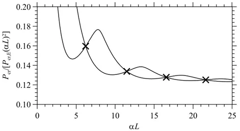
Normalized critical loads turn out to be proportional to the square of the beam-subgrade parameter αL. Fig. 1.8c shows the ratio Pcr/[Pcr,E (L)2] versus the

parameter αL; for increasing αL, the ratios corresponding to the first and second smallest eigenvalues converge to a constant value equal to 0.121, this value is coincident with the coefficient obtained in Eq. 1.27. Comparing the numerical solution with the one determined by Reissner (1937), for αL values up to 5 (short beams and/or soft soil), the numerical solution is in good agreement with Eq. 1.26, whereas for the high values of αL (long beams and/or stiff soil) the numerical solution is well approximated by Eq. 1.27.

(a) 0x10 0 2x103 4x103 6x103 8x103 104 L3 0 10 20 30 40 50 P/Pcr cr ,E (b) 0 5 10 15 20 25 L 0 10 20 30 40 50 P/Pcr cr ,E (c) 0 5 10 15 20 25 L 0 0.1 0.2 0.3 0.4 0.5 P/[cr Pcr ,E ( L ) 2] 0.121

Fig. 1.8 – Dimensionless critical loads Pcr (continuous lines) and Pcr,m (dashed lines) versus

αL for a beam with sliding ends.

The curves in Figs. 1.8a, b and c, exhibit curve veering and crossing points which interchange themselves for increasing values of L. The coordinates of crossing points can be determined approximately by refining the L values in

the coordinates of the first four crossing points for the first two curves, which are also depicted with crosses in Fig. 1.9.

Point 1 2 3 4 αL 6.232 11.735 16.573 21.633

Pcr/Pcr,E 6.200 17.511 35.092 58.546

Tab. 1.3 – Coordinates of the first four crossing points between the first and second eigenvalues for a beam with sliding ends on elastic half-plane.

0 5 10 15 20 25 L 0.10 0.12 0.14 0.16 0.18 0.20 P/[cr Pcr, E ( L ) 2]

Fig. 1.9 – First and second critical loads of a beam with sliding ends on elastic half-plane (continuous lines) with the first four crossing points (crosses).

The behaviour of a beam with sliding ends on elastic half plane is found to be quite analogous to a beam with sliding ends resting on Winkler soil (Hetenyi 1946; Timoshenko and Gere 1961; Bazant and Cedolin 1991),where coordinates of intersection points may be exactly known, but curve veering is not present. Moreover, the curve representation shown in Figs. 1.8a, b and c, was introduced for the first time by Ratzersdorfer (1936) for the case of the beam on Winkler soil.

1.5.2.1 Modal shapes

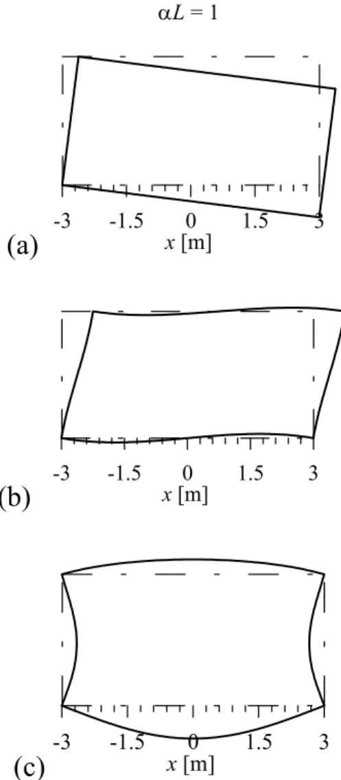
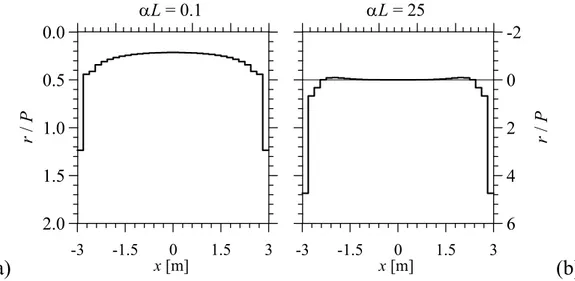
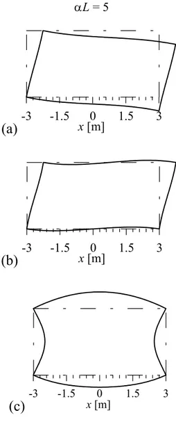
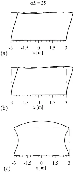
The modal shapes of a beam with sliding ends on elastic half-plane turn out to be sinusoidal. The number of half-waves and their amplitude depends on the αL parameter. In the following figures, modal shapes are shown for increasing αL values; displacements are normalized putting the maximum absolute beam deflection equal to 1; moreover, the corresponding soil reactions are shown.

(a) -0.5 0.0 x/L 0.5 1 0 -1 v L = 5 L = 10 -0.5 0.0 x/L 0.5 1 0 -1 v (b) (c) -0.5 0.0 x/L 0.5 10-2 10-2 r -0.5 0.0 x/L 0.5 10-3 10-3 r (d)

Fig. 1.10 – First (continuous line) and second (dashed line) mode shapes for a beam with sliding ends and L equal to 5 (a), 10 (b). Soil reactions corresponding to the first (continuous

line) and second (dashed line) mode shapes for a beam with sliding ends and L equal to 5 (c), 10 (d).

For αL = 5, Fig. 1.10a shows the first two mode shapes which are characterized by one and two half-waves; whereas, for αL = 10, two and three half-waves are observed (Fig. 1.10b). Fig. 1.10c and d show the corresponding soil reactions. For αL = 10, the first mode shape (Fig. 1.10b, continuous line) is similar to the second one obtained for αL = 5 (Fig. 1.10a, dashed line), however, the second

if the first and second critical load curves (Figs. 1.8a, b and c) interchange themselves, the corresponding buckling modes do not interchange each other. For αL = 15 and 20, Figs. 1.11a and b show the first two mode shapes, respectively, whereas Figs. 1.11c and d show the corresponding soil reactions. The first mode shape for αL = 15 is characterized by three half-waves and for αL = 20 it is characterized by four half-waves. Hence, after each intersection point (Tab. 1.3), every mode shape changes and the number of half-waves increases.

(a) -0.5 0.0 x/L 0.5 1 0 -1 v L = 15 L = 20 -0.5 0.0 x/L 0.5 1 0 -1 v (b) (c) -0.5 0.0 x/L 0.5 10-4 10-4 r -0.5 0.0 x/L 0.5 10-4 10-4 r (d)

Fig. 1.11 – First (continuous line) and second (dashed line) mode shapes for a beam with sliding ends and L equal to 15 (a), 20 (b). Soil reactions corresponding to the first (continuous line) and second (dashed line) mode shapes for a beam with sliding ends and L

equal to 15 (c), 20 (d).

Figs. 1.10, 1.11 and 1.12 clearly show that for increasing αL, the number of half-waves for the first two mode shapes increases and short wavelengths are obtained. Furthermore, mode shapes amplitude is not constant and for increasing αL it tends to reach maximum values close to beam midpoint. A different behaviour can be detected in beam on Winkler soil (Timoshenko and Gere 1961;

Bazant and Cedolin 1991), where mode shapes amplitude is constant, as shown in the following paragraph.

(a) -0.5 0.0 x/L 0.5 1 0 -1 v L = 25 L = 50 -0.5 0.0 x/L 0.5 1 0 -1 v (b) (c) -0.5 0.0 x/L 0.5 10-4 10-4 r -0.5 0.0 x/L 0.5 10-5 10-5 r (d)

Fig. 1.12 – First (continuous line) and second (dashed line) mode shapes for a beam with sliding ends and L equal to 25 (a), 50 (b). Soil reactions corresponding to the first (continuous line) and second (dashed line) mode shapes for a beam with sliding ends and L

equal to 25 (c), 50 (d).

The critical wavelength cr,R of the sinusoidal waveform assumed by Reissner

(1937) is equal to (Volynskii et al, 2000):

        2 4 9.97 3 2 3 0 3 R cr, E E h , (1.31)

where direct proportionality between the wavelength cr,R and the thickness h of

the beam is predicted. Eq. 1.31 was used in advanced metrology methods to measure the elastic modulus of polymeric thin film (Stafford et al, 2004). Excluding the half-waves close to beam ends, the present analysis predicts a

checked. Thus, the eigenvectors shown in Fig. 1.12b have almost-constant wavelength and variable amplitude, unlike the mode shape assumed in Reissner 1937 (Eq. 1.21), which is sinusoidal with constant amplitude and wavelength.

1.5.2.2 Beam with sliding ends on Winkler-type half-space

The analysis of a beam resting on a Winkler-type half space (1867) is briefly described in the appendix A2. It is well known that the idealized model of half-space proposed by Winkler assumes that the deflection v at a point of the surface is directly proportional to the stress or soil pressure r applied at the same point and independent of stresses applied at other locations:

) ( )

(x c v x

r   (1.32)

where c is a constant known as Winkler constant or modulus of subgrade reaction.

Critical loads of a beam with sliding ends on Winkler-type soil are equal to critical loads of a beam with pinned ends and are given by (Hetenyi 1948, Bazant and Cedolin 1991, Wang et al. 2005):

          2 ₂2 ₄ E cr, W cr, m m P P for m = 1, 2, 3, ... (1.33) where b D L c 4   (1.34)

describes the beam-subgrade system for the Winkler-type half-space and it corresponds to αL parameter for the beam resting on half-plane.

Considering the beam discrete model described in §1.3 and applying it to the case of a beam on Winkler-type soil (as shown in the appendix A2), critical loads may be determined and compared with the analytic solution (Eq. 1.33). Figs. 1.13a and b show dimensionless critical loads Pcr/Pcr,E, determined with the

discrete model adopted, for increasing γ2 and γ, respectively. Results turn out to be coincident with the analytic solution (Fig. 1.13b).

(a) 0 5000 10000 15000 20000 25000  0 15 30 45 60 Pcr /P cr ,E (b) 0 50 100 150 200  0 15 30 45 60 Pcr /P cr ,E (c) 0 50 100 150 200  0 0.2 0.4 0.6 Pcr /( Pcr ,E  ) 2/2

Fig. 1.13 – Dimensionless critical loads Pcr (continuous lines) and Pcr,W (circles) versus γ for a

Fig. 1.13c shows that dimensionless critical loads are proportional to γ and the smallest critical load tends to:

2 E cr, min W, cr, 2    P P , (1.35)

which can also be obtained from Eq. 1.33.

The behaviour showed in Figs. 1.13a, b and c is quite similar to the one obtained for the beam on elastic half-plane. In this case, however, curves present crossing points but curve veering is not present. Minimum critical load Pcr,W,min for

increasing γ (Eq. 1.35) may be compared with the corresponding one of the beam on half-plane Pcr,R (Eq. 1.27). Then, a ratio between the modulus of

subgrade reaction c and half plane modulus E can be determined:

1/3 1/3 4 4 4 4 2 cr,E 2 cr,E 3 2 14/3 2 3 _{( )} 9 _0.354 2 16 _{b b} E b E b P P L c D D                         . (1.36)

The coefficient in Eq. 1.36 is larger than the one obtained by Biot (1937), who determined the relation between the foundation modulus c and the half plane modulus E in order to obtain the same maximum bending moment of an infinite beam loaded by a concentrated force at midpoint:

1/3 1/3 4 4 4 4 4/3 0.710 _0.282 2 _{b b} E b E b c D D                   . (1.37)

However, if results showed in Figs. 1.13a, b and c are scaled taking into account Eq. 1.36, minimum critical loads tend to be coincident with the ones obtained for the beam on elastic half-plane for large values of αL (Fig. 1.14).

Figs. 1.15a and b show the first and second mode shapes for γ equal to 15 and 400, which correspond to αL close to 5 and 25, respectively (Eq. 1.36). For the case of a beam resting on soft support (Fig. 1.15a), the first and second mode shapes are characterized by one and two half-waves, respectively, and they are almost coincident with results obtained for the beam resting on half-plane (Fig. 1.10a). For a beam resting on stiff support (Fig. 1.15b), the first and second mode shapes are sinusoidal with constant wavelength and amplitude, whereas the corresponding case for beam resting on half-plane is characterized by sinusoidal mode shapes with different amplitude along beam length (Fig. 1.12a).

0 5 10 15 20 25 L 0 0.1 0.2 0.3 0.4 0.5 P/[cr Pcr, E ( L ) 2] 0.121

Fig. 1.14 – Dimensionless critical loads Pcr for a beam with sliding ends on elastic half plane (continuous lines) and on Winkler half-space (dots).

(a) 1 0 -1 v  = 400 -0.5 0 x/L 0.5  = 15 -0.5 0 x/L 0.5 1 0 -1 v (b)

Fig. 1.15 – First (continuous line) and second (dashed line) mode shapes for a beam with sliding ends on Winkler-type half-space for γ = 15 (a) and 400 (b).

1.5.3 Beam of finite length with pinned ends

The case of a foundation beam with pinned ends (Fig. 1.16) may refer to a rigid portal frame whose columns are hinged to the foundation beam; thus, the structure enforces zero relative displacement between beam ends, but allows independent rotations.

P

P

L

Fig. 1.16 – Beam with pinned ends subject to axial load P.

It is worth noting that the constraint equations must not be the typical equations of a beam with simple supported ends R1 = v(L/2) = 0, R2 = v(L/2) = 0, because

the behaviour of a beam on 2D half-plane is always characterized by a rigid body displacement, which cannot be set equal to zero a priori. Then, the constraint equation that has to be applied to Eq. 1.6 is R1 = v(L/2)  v(L/2) = 0.

Adopting a penalty parameter k = 106 Db/L3, an error less than 10-3 is obtained

for the first ten eigenvectors.

In Figs. 1.17a and b, the first seven dimensionless buckling loads Pcr/Pcr,E are

plotted versus the parameter L3 _{and L, respectively. For αL = 0, numerical}

results coincide both with critical loads of a beam with pinned ends and with analytic solutions given by Reissner’s solution (Eq. 1.26), moreover for low L values, numerical results are quite close to Reissner’s solution (dashed lines). For increasing L, Figs. 1.17a and b show that the first and second critical loads tend to separate from other critical loads and the corresponding values are lower than Eq. 1.26, which correspond to the values obtained for the beam with sliding ends.

On the other hand, the third and fourth eigenvalues remain close to Reissner’s solution (dashed lines), and the curves after the third one are characterised by veering and crossing points, similarly to the previous case of a beam with sliding ends.

(a) 0x10 0 2x103 4x103 6x103 8x103 104 L3 0 10 20 30 40 50 P/Pcr cr ,E (b) 0 5 10 15 20 25 L 0 10 20 30 40 50 P/Pcr cr ,E (c) 0 5 10 15 20 25 L 0 0.1 0.2 0.3 0.4 0.5 P/[cr Pcr, E ( L ) 2] 0.121 0.106 0.083

Fig. 1.17 – Dimensionless critical loads Pcr (continuous lines) and Pcr,m (dashed lines) versus

Fig. 1.17c shows the ratio Pcr/[Pcr,E (L)2] versus the parameter αL; for

increasing αL the first and the second eigenvalues converge to:

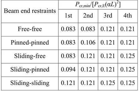
2 E cr, cr,1 0.083P (αL) P  , (1.38) 2 E cr, cr,2 0.106P (αL) P  , (1.39)

whereas the third and fourth critical loads turn out to be very close to Reissner’s solution and converge to Eq. 1.27. Therefore, the existence of critical loads lower than Pcr,R in Eq. 1.27 is clearly shown. In particular, Eqs. 1.38 and 1.39

yield the following critical stresses:

3 / 1 0 3 / 2 cr,1 cr,1 0.36E E h b P    . (1.40) 3 / 1 0 3 / 2 cr,2 cr,2 0.46E E h b P    . (1.41)

1.5.3.1 Modal shapes (a) -0.5 0.0 x/L 0.5 1 0 -1 v L = 5 L = 10 -0.5 0.0 x/L 0.5 1 0 -1 v (b) (c) -0.5 0.0 x/L 0.5 10-2 10-2 r -0.5 0.0 x/L 0.5 10-3 10-3 r (d)

Fig. 1.18 – First (continuous line) and second (dashed line) mode shapes for a beam with pinned ends and L equal to 5 (a), 10 (b). Soil reactions corresponding to the first (continuous

line) and second (dashed line) mode shapes for a beam with pinned ends and L equal to 5 (c), 10 (d).

For αL = 5, Fig. 1.18a shows that the first and second mode shapes present one and two half-waves, respectively, and they are clearly sinusoidal. For αL = 10 (Fig. 1.18b) the first mode shape is quite different from the one obtained for αL = 5 and it can not be described by a sine or cosine function, while the second mode shape is, indeed, sinusoidal with two half-waves. The difference between the first mode shapes obtained for αL = 5 and 10 can be described considering Figs. 1.17a and b. For αL = 5, the first and second critical loads are still in good agreement with Reissner’s solution (Eq. 1.26), whereas for αL = 10 the first critical load is lower than Eq. 1.26.

(a) -0.5 0.0 x/L 0.5 1 0 -1 v L = 15 L = 20 -0.5 0.0 x/L 0.5 1 0 -1 v (b) (c) -0.5 0.0 x/L 0.5 10-4 10-4 r -0.5 0.0 x/L 0.5 10-4 10-4 r (d)

Fig. 1.19 – First (continuous line) and second (dashed line) mode shapes for a beam with pinned ends and L equal to 15 (a), 20 (b). Soil reactions corresponding to the first (continuous line) and second (dashed line) mode shapes for a beam with pinned ends and L

equal to 15 (c), 20 (d).

For increasing αL (Figs. 1.19a and b), half-waves cannot be easily defined like in previous cases and buckling modes have large amplitudes near beam ends. Indeed, the critical loads in Eqs. 1.38 and 1.39 correspond to these localized buckling modes. It is interesting to note that the first mode shapes shown in Figs 1.18-1.20 are symmetric, whereas the second mode shapes are antisymmetric and, in fact, the first and second curves in Figs. 1.17a, b and c do not have any intersection point.

(a) -0.5 0.0 x/L 0.5 1 0 -1 v L = 25 L = 50 -0.5 0.0 x/L 0.5 1 0 -1 v (b) (c) -0.5 0.0 x/L 0.5 10-4 10-4 r -0.5 0.0 x/L 0.5 10-5 10-5 r (d)

Fig. 1.20 – First (continuous line) and second (dashed line) mode shapes for a beam with pinned ends and L equal to 25 (a), 50 (b). Soil reactions corresponding to the first (continuous line) and second (dashed line) mode shapes for a beam with pinned ends and L

(a) -0.5 0.0 x/L 0.5 1 0 -1 v L = 5 L = 10 -0.5 0.0 x/L 0.5 1 0 -1 v (b) (c) -0.5 0.0 x/L 0.5 1 0 -1 v L = 25 L = 50 -0.5 0.0 x/L 0.5 1 0 -1 v (d)

Fig. 1.21 – Third (continuous line) and fourth (dashed line) mode shapes for a beam with pinned ends and L equal to 5 (a), 10 (b), 25 (c) and 50 (d).

The first and second eigenvectors are different than the following ones, in fact Figs. 1.21a-d show the third and fourth mode shapes for increasing αL values, which are sinusoidal with increasing half-waves number and varying amplitude along beam length. For αL = 25 and 50 (Figs. 1.21c, d), the third and fourth mode shape, excluding deformations at beam ends, are quite similar to the first and second mode shapes obtained for the beam with sliding ends (Figs. 1.12a and b). Then, the behaviour of a beam with pinned ends on elastic half-space is found to be quite different from the previous case of beams with sliding ends, which does not present localized eigenmodes for increasing values of αL (long beam and/or stiff soil).

As for Winkler soils, reference is usually made to Hetenyi (1946), where the solution of the beam with pinned ends converges to the same critical load of the beam with clamped ends (Hetenyi 1946, Simitses 1976). Nonetheless, for beams

on Winkler soil with pinned ends, Goodier and Hsu (1954) reported the presence of mode shapes localized at beam ends.

1.5.3.2 Bosakov’s solution (1994)

The stability of a beam with pinned ends resting on elastic half-plane was studied by Bosakov (1994) by adopting symmetric cosine functions:

           ( , ,0) ) 1 2 ( ) α ( 2 ) 1 2 ( ₃ 3 2 E cr, B cr, F m m m L m P P for m = 0, 1, 2, ... (1.42)

where F(m, m, 0) is a function reported in the original paper (Bosakov 1994), based on Bessel functions of the first kind. Eq. 1.42 is compared with critical loads obtained with the present model and results are shown in Figs. 1.22a and b. (a) 0 5 10 15 20 25 L 0 10 20 30 40 50 P/Pcr cr ,E (b) 0 5 10 15 20 25 L 0 0.1 0.2 0.3 0.4 0.5 P/[cr Pcr ,E ( L ) 2] 0.121 0.106 0.083

Fig. 1.22 – Dimensionless critical loads Pcr (continuous lines), Pcr,m (dashed lines) and Pcr,B

The first buckling load is well approximated by Eq. 1.42 for αL < 7 (see dots in Figs. 1.22a and b), and by Eq. 1.26 for αL < 3. Moreover, Figs. 1.22a, b and c show that Eq. 1.42 is unable to provide eigenvalues corresponding to antisymmetric buckling and for large values of αL, as Bosakov’s solution is not able to provide the first and second critical loads obtained with the present model.

1.5.3.3 Gallagher’s solution (1974)

Another solution for the buckling of a beam with pinned ends under axial compression on elastic half-plane was determined by Gallagher (1974). The solution is based on Chebyshev polynomials of the first and second kind:

  r T_r cos ,     sin ] ) 1 sin[(r U_r (1.43a,b)

and considering separately the even modes (Eq. 1.44) and the odd modes (Eq. 1.45) of buckling.





where  2x /L and prime represents differentiation with respect to x.

The relation between beam displacement and half-space pressure considered by Gallagher is given by the following relation (Muskhelishvili 1963):

x d x x x L x v x L E x r L L ˆ ) ˆ ( ˆ 4 ) ˆ ( ' 4 2 ) ( 2 / 2 / 2 2 2 2 0





Gallagher adopted the same beam-subgrade parameter αL considered in the present model and determined numerically the first six eigenvalues by substituting Eqs. 1.44, 1.45 and 1.46 in the differential equation of the beam on elastic half-plane with second order effects due to the axial load P. The author stopped the series in Eqs. 1.44 and 1.45 at n = 36 and found a linear relationship between critical loads and αL3, but only for certain ranges of αL, depending on

the mode. Moreover, considering even modes and odd modes separately, the curves corresponding to dimensionless critical loads (λ, αL3 or λ, αL) never intersect. However, for simplicity, the following relation between critical loads and αL was adopted to describe the results:

         Cm L m P P ₂ 3 2 E cr, G cr, 2 ) α ( for m = 1, 2, 3, ... (1.47)

where Cm is a constant depending on the mode number; the values of

m

C m _/2)2

(  are listed in Tab. 1.4 for the first six buckling modes.

m 1 2 3 4 5 6 m C m 2 2 _      _{1.05 1.77 2.66 3.39 4.23 4.97} Tab. 1.4 – Values of ₍m_/2)2C_m

for the first six buckling modes (Gallagher 1974).

Figs. 1.23 a, b and c show critical loads given by Eq. 1.47 with triangles, and these results are compared with the ones obtained with the present model for the same beam case (continuous lines, as already shown in Figs. 1.17a, b and c). It is clear that Pcr,G (Eq. 1.47) for m = 1, 2 does not converge to the first and second

eigenvalues obtained with the present model, but it converges to the third and fourth eigenvalues. Moreover, Fig. 1.23c clearly shows that minimum values of

(a) 0x10 0 2x103 4x103 6x103 8x103 104 L3 0 10 20 30 40 50 P/Pcr cr ,E (b) 0 5 10 15 20 25 L 0 10 20 30 40 50 P/Pcr cr ,E (c) 0 5 10 15 20 25 L 0 0.1 0.2 0.3 0.4 0.5 P/[cr Pcr,E ( L ) 2] 0.121 0.106 0.083

Fig. 1.23 – Dimensionless critical loads Pcr (continuous lines) and Pcr,G (triangles) versus αL

for a beam with pinned ends.

The critical loads determined by Gallagher are found to be very close to the ones obtained for the case of a beam with sliding ends. Figs. 1.24a and b show Pcr,G

(Eq. 1.47) with triangles which are practically coincident with the dimensionless critical loads already shown in Figs. 1.8b and c (continuous lines). The solution

proposed by Gallagher is not able to describe the buckling localized at beam ends (Figs 1.20a and b), which characterizes the first and second critical loads for increasing αL. (a) 0 5 10 15 20 25 L 0 10 20 30 40 50 P/Pcr cr ,E (b) 0 5 10 15 20 25 L 0 0.1 0.2 0.3 0.4 0.5 P/[cr Pcr, E ( L ) 2] 0.121

Fig. 1.24 – Dimensionless critical loads Pcr (continuous lines) for a beam with sliding ends

and Pcr,G (triangles) versus αL for a beam with pinned ends.

1.5.3.4 Beam with pinned ends on Winkler-type half-space

The most known solution for the buckling of a beam with pinned ends on Winkler-type half-space is coincident with the one defined for the beam with sliding ends (Eq. 1.33, Hetenyi 1948, Timoshenko and Gere 1961, Wang et al. 2005). However, this solution is obtained by satisfying the boundary condition

0 ) 2 / ( ) 2 / (L v L 

(a) 0 5000 10000 15000 20000 25000  0 15 30 45 60 P /Pcr cr ,E (b) 0 50 100 150 200  0 15 30 45 60 P /Pcr cr ,E (c) 0 50 100 150 200  0 0.2 0.4 0.6 Pcr /( Pcr ,E  ) 2/2 1/2

Fig. 1.25 – Dimensionless critical loads Pcr versus γ for a beam with pinned ends on

Winkler-type half space.

If the condition v(L/2)v(L/2) is adopted, critical loads turn out to be different than Eq. 1.33. Figs. 1.25 a and b show dimensionless critical loads

Pcr/Pcr,E, determined with the discrete model adopted, for increasing γ2 and γ,