Absolute Proper Motions Outside the Plane (APOP) - A Step Toward the GSC2.4

2020-04-18T10:11:10Z

Acceptance in OA@INAF

Absolute Proper Motions Outside the Plane (APOP) - A Step Toward the GSC2.4

Title

Qi, Zhaoxiang; Yu, Yong; BUCCIARELLI, Beatrice; LATTANZI, Mario Gilberto;

SMART, Richard Laurence; et al.

Authors

10.1088/0004-6256/150/4/137

DOI

http://hdl.handle.net/20.500.12386/24099

Handle

THE ASTRONOMICAL JOURNAL

Journal

150

ABSOLUTE PROPER MOTIONS OUTSIDE THE PLANE

(APOP)—A STEP TOWARD THE GSC2.4

Brian J. McLean3, Zhenghong Tang1, Hugh R. A. Jones4, Roberto Morbidelli2, Luciano Nicastro5, and Alberto Vecchiato2

1

Shanghai Astronomical Observatory, Chinese Academy of Sciences, 80 Nandan Road, 200030 Shanghai, China 2

INAF—Osservatorio Astrofisico di Torino, Strada Osservatorio 20, I-10025 Pino Torinese, TO, Italy 3

Space Telescope Science Institute, 3700 San Martin Drive, Baltimore, MD 21218, USA 4

Centre for Astrophysics Research, University of Hertfordshire, Hatfield AL10 9AB, UK 5

INAF—Istituto di Astrofisica Spaziale e Fisica Cosmica, via Piero Gobetti, 101, I-40129, Bologna, Italy Received 2014 December 10; accepted 2015 June 14; published 2015 October 6

ABSTRACT

We present a new catalog of absolute proper motions and updated positions derived from the same Space Telescope Science Institute digitized Schmidt survey plates utilized for the construction of Guide Star Catalog II. As special attention was devoted to the absolutization process and the removal of position, magnitude, and color dependent systematic errors through the use of both stars and galaxies, this release is solely based on plate data outside the galactic plane, i.e., b∣ ∣ 27. The resulting global zero point error is less than 0.6 mas yr−1, and the precision is better than 4.0 mas yr−1 for objects brighter than RF= 18.5, rising to 9.0 mas yr−1 for objects with

magnitudes in the range 18.5< RF< 20.0. The catalog covers 22,525 square degrees and lists 100,774,153 objects

to the limiting magnitude of RF∼ 20.8. Alignment with the International Celestial Reference System was made

using 1288 objects common to the second realization of the International Celestial Reference Frame (ICRF2) at radio wavelengths. As a result, the coordinate axes realized by our astrometric data are believed to be aligned with the extragalactic radio frame to within±0.2 mas at the reference epoch J2000.0. This makes our compilation one of the deepest and densest ICRF-registered astrometric catalogs outside the galactic plane. Although the Gaia mission is poised to set the new standard in catalog astronomy and will in many ways supersede this catalog, the methods and procedures reported here will prove useful to remove astrometric magnitude- and color-dependent systematic errors from the next generation of ground-based surveys reaching significantly deeper than the Gaia catalog. Key words: astrometry– astronomical databases: miscellaneous – catalogs – proper motions – reference systems

1. INTRODUCTION

The Second Generation Guide Star Catalog, or GSC-II, is an all-sky catalog of objects built from the Digitized Sky Surveys that the Space Telescope Science Institute(STScI) created from the Palomar and UK Schmidt survey plates (GSC2.3, Lasker et al. 2008). The GSC-II was primarily created to continue providing guide star information6 and observation planning support, including protection from nearby bright objects to the new generation ultra-sensitive cameras installed on the Hubble Space Telescope (HST) since the first GSC. Thanks to its relatively faint magnitude limit and multi-band photometry, GSC-II is also employed at some of the largest ground-based facilities such as GEMINI, the Very Large Telescope, and LAMOST. In the most recent version (GSC2.3.4 in HST operations), it was found that the derived proper motions, although compliant with the Hubble operations, suffered from significant systematic errors, especially in the southern hemi-sphere, and for this reason they were not included in the version released to the astronomical community. This limited the scientific and also technical (e.g., accurate operation of multi-fiber spectrographs) usefulness of the public GSC2.3; various experiments were then initiated to investigate the sources of such systematic errors and to explore alternative methods for improving the proper motion accuracy (Spagna et al.2004; Tang et al.2008). Astrophysically, large samples of accurate absolute proper motions to faint magnitudes are

fundamental observables in Milky Way studies to gain, e.g., further insight into the recently discovered evidence of unexpected chemo-kinematical features (Spagna et al. 2010). These newfindings bear the potential to shed new light on the origin and evolution of our Galaxy(Curir et al. 2012,2014), and ultimately on its role in cosmology(Lattanzi2012).

In this paper we concentrate on the recalibration of the GSC-II proper motions; however, we also discuss the catalog release (which includes a recalibration of the positions); the catalog, in the form presented here, will be made available at the Strasbourg astronomical Data Center(CDS) with the publica-tion of this article.

Assuming we can consider the proper motions of galaxies to be zero, there are two ways to exploit this in the determination of absolute proper motions.

1. One is the direct way; here, all the observations obtained at different epochs are directly transformed into one system using galaxies as reference objects; therefore, absolute proper motions are a natural derivation within this approach.

2. The other possibility is to bring all the observations into a common system using stars (instead of galaxies) as reference objects from which to calculate relative proper motions of all of the measured objects. Then, render those proper motions absolute by subtracting the pseudo proper motions of the galaxies.

The GSC-II object classification is based on star/non-star criteria rather than star/galaxy. This was done for operational

© 2015. The American Astronomical Society. All rights reserved.

6 _{In this respect, GSC-II includes thefirst generation GSC, or GSC-I (Lasker} et al.1990).

reasons in order to prioritize the reliability of the star classification at the cost of a less accurate, more generic, non-star classification. Therefore, non-stars will be a mix of blended objects, faint stars, and galaxies, providing a heterogeneous reference system. This mixing is not easy to disentangle, leading to imprecise astrometric transformations; furthermore, the individual accuracy of the measured positions for the non-stars is generally worse than that for stars. Therefore, after a number of dedicated evaluation tests, we decided to adopt the second procedure.

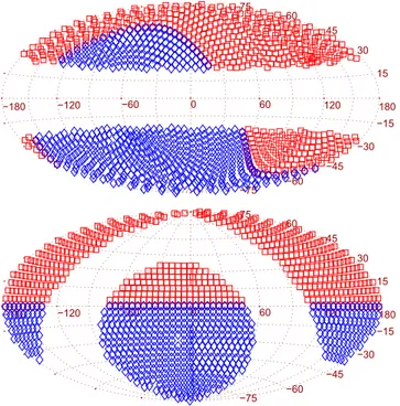
Due to increasing interstellar extinction as we approach the galactic plane, the number of observable (genuine) galaxies drops to zero. In the end, our reductions only addressed the parts of the celestial sphere with galactic latitudes b∣ ∣ 27; see Figure1. This is only an operational definition of off-the-galactic-plane regions, and clearly depends on the lack of non-stars for our reductions below that latitude.

The next section describes the plate data used to derive the proper motions in our catalog, which we decided to call “Absolute Proper motions Outside the Plane,” or APOP, for brevity.

In the 3rd section we present the calibration pipeline and the details of the detection and removal of systematic errors that are dependent on plate position, magnitude, and color (hereafter PdE, MdE, and CdE, respectively).

In Section 4, the anticipated precision is estimated theoretically, and both internal and external precisions are assessed. This section also describes the APOP available to the community through the CDS center in Strasbourg. Finally, the last section presents some conclusions and briefly discusses future plans.

2. PLATE DATA

The observational data come from the STScI Catalog of Objects and Measured Parameters from All-Sky Surveys (COMPASS) archive of the GSC-II project (see Lasker et al.1998). This object-oriented database is the repository of the original(raw) measurements (astrometric and photometric) of all of the objects detected on any of the 9000+ survey plates digitized at STScI; it also contains the entire set of parameters resulting from all of the plate-based calibrations (object detection and inventorying, astrometry, photometry, and image classification). Below we summarize the properties of the data in the COMPASS repository that are useful for better understanding the next sections (precise references to the relevant parts of the 2008 work of Lasker et al., or other published papers, are provided whenever appropriate):

1. Sky coverage and epochs. The different photographic plate collections inventoried in COMPASS cover all directions of the celestial sphere at least a few times over the timespan they comprise. The Northern declinations were observed with time differences that span from a minimum of∼25 years to as much as 50 years. For the Southern sky the situation is distinctively less homo-geneous: for the declinations in common with those reached by the Palomar Observatory Schmidt telescope first epoch campaigns (δ … −30°), epoch differences can extend to 50 years; however, intervals as short as a few years can occur further South. The details of the decl. ranges reached by each individual Schmidt plate survey and the corresponding epoch intervals are in Table 1 of Lasker et al.(2008);

2. Photometric bands. Table 1 of Lasker et al.(2008), along with their Figure 1, provides information on the photometric data in COMPASS. In particular, the relation of the photographic passbands RF, BJ, IN with the

Johnson–Kron-Cousins B V R Ic photometric system is

clearly illustrated, with BJsignificantly extending into the

wavelength range of the photometric V. Although only BJ

and RF magnitudes are explicitly utilized in this article,

all of the GSC-II based photographic magnitudes are listed with the APOP entries(see Table 1 in Section4.4); 3. Cross-identification of the same objects detected on different plates was made using a matching radius of 4 arcsec;

4. The digitized resolution of most plates is 15μm/pixel (1 arcsec/pixel), while some plates were scanned at 25μm/pixel (1.7 arcsec/pixel; details in Table 1 of Lasker et al.2008);

5. Errors. The average error of the measured plate coordinates is about 0.12–0.13 pixel at intermediate magnitudes, i.e., brighter than 18.5(Spagna et al.1996); also, the average photometric error is within 0.13–0.22 mag(16 mag < RF< 20 mag);

6. GSC2.3 Classification. The reliability of star classifica-tion remains above 90% to RF = 19.5, and better than

95% to RF = 18.5, while that of non-stars classified as

galaxies is significantly less (Right panel of Figure 29 in Lasker et al.2008), with numbers always below 85% and to a low of 70% at the faint limit.

The success of the procedures we have adopted for the APOP construction relies heavily on the accuracy of the classification of both stars and galaxies. Besides, as already

Figure 1. Sky distribution of the Schmidt plates used in the APOP catalog. There are 4239 plates used in the reductions. The total area covered by this catalog is 22,525 deg2_{. The topfigure represents the celestial sphere in Galactic} coordinates and the bottom is its analog in Equatorial coordinates. The blue diamonds represent plates withδ < 0° and the red squares those with δ … 0°.

stated in the previous section and quantified in the last of the GSC2.3 properties above, classification is limited to star/non-star, with no galaxy class, which complicates the calculation of absolute proper motions. Therefore, before going into the details of the astrometric calibration algorithms discussed in Section3, these are two facts that are important to clarify here. First, the error of the measured coordinates and the property of accurately classifying stars to 95% confidence down to RF= 18.5 completely justifies the 16 < RF< 18.5 mag range

as the interval of choice for the reference (anonymous) stars utilized in the initial plate-to-plate astrometric reductions. Then, the precise knowledge that the classification of non-stars as galaxies is significantly less reliable was the motivation for developing the new procedure to iteratively refine the selection of genuine galaxies from the non-star objects for improvedfinal astrometric calibrations and proper motion absolutization.

3. CATALOG CONSTRUCTION

There are three critical factors affecting errors of absolute proper motions: (a) the epoch range spanned by the survey plates employed, (b) the quality (e.g., intrinsic noise) of the emulsions of that same photographic material along with that of the measuring machines utilized for the digitization process, and(c) the modeling of the transformation of plates of different epochs to a common reference frame. The third element is really the only one we can work on to improve the calibrations and hopefully derive better proper motions.

It is well known that because of the combined influence of the atmosphere (differential refraction, dispersion, extinction etc.), telescope (guiding errors, distortion of field of view, etc.), photographic plates (uneven response to bending stress, size and distribution of emulsion, low quantum efficiency etc.), and plate scanner(digitizing errors), individual plate coordinates of the detected objects, as well as their magnitudes and colors, can have varied systematic errors that are dependent on the position, magnitude and color of the same objects, and these systematics can be different for the different survey plates(see for example Taff et al. 1990; Morrison et al. 1998; Evans & Irwin1995; Kuimov et al.2000).

As proper motions are derived from positions at different epochs, it is likely that they will suffer from similar systematic errors. On the other hand, actual(physical) proper motions are expected to exhibit correlations with sky direction, magnitude and color due to the motions of the different stellar populations within the Milky Way. Therefore, one aspect that must be carefully considered when attempting the elimination of the systematic errors mentioned above is not to bias the proper motions with unphysical sources.

Below, we describe both the reduction procedures and assumptions adopted.

3.1. Principles of Calibration

Following the work by van Altena et al.(1990), Spagna et al. (1996), and, more recently, by Mahmud & Anderson (2008), Kallivayalil et al.(2013) and Pryor et al. (2014), we work under the hypothesis that the absolute proper motions of galaxies are always zero, i.e., they are not dependent on their plate position, magnitude, or color. To this we add a second hypothesis: objects(stars and galaxies) physically close on a photographic plate and with similar magnitudes/colors have similar systematic errors.

Based on these assumptions, and considering the available plate data, the adopted procedure is to choose a good quality plate as the reference plate and to use the objects classified as stars with good image quality to transform the relevant program plates to the reference plate system. Here good image quality means objects in the middle of the unsaturated magnitude range (i.e., 16.0 < RF < 18.5) where the centering errors are

minimized, i.e.∼0.13 arcsec, see Section2. The major plate-based calibration steps are:

1. Remove the PdE with a moving-meanfilter7using stellar objects with good image quality;

2. Select galaxies from non-stars via their pseudo(common) motion relative to the reference stars; and

3. Calibrate the MdE, CdE and the residual PdE of all objects with reference to the galaxies.

Finally, absolute proper motions are calculated from all of the detections at the different plate epochs.

The relevant equations are described below.

For each object, the difference of positions between the reference(plate 1) and one of the corresponding program plates (plate 2) is modeled as x x x t D x y E m c x y , , , , 1 x s 1 2 2 2 2 2 2 2 ( ) ( ) ( ) m D = - = D + + xg D x( 2,y2) E m( 2,c2,x2,y2), ( )2 D = +

where Δxs,Δxgrepresent the individual positional difference

of stars and galaxies, respectively, and μxis a star’s absolute

proper motion in the reference plate coordinate system; also,Δt is the epoch interval between the reference and program plates, D is the PdE, and E is the combined MdE and CdE. Similar equations hold for the y coordinate.

The absolute proper motionμxof each star can be separated

into the average proper motionsm for all reference stars on the¯_x plate and a remaining individual proper motion, relative to the reference stars, dμx, i.e.,

d . 3

x ¯x x ( )

m = m + m

Removing the systematic error D, besides removing the average MdE and CdE of the reference stars, also removes their average proper motions m , while the galaxies will attain a¯_x “pseudo” proper motion- .m¯x

After this step, the position differencesD ¢ D ¢ of starsxs, xg and galaxies between the reference and program plates can be expressed as: x x x x D t d t E 4 x x s 1 2 s

(

)

(

)

Equation(5) has a special role in our reduction procedure; we iterate exactly on this equation to reject non-stars that are not genuine galaxies. In practice, assuming that all real galaxies will show the common pseudo proper motion-m¯_x discussed before, weflag as outliers, i.e., probable blended objects, those that do not.8In the end, the selected true galaxies constrain the average proper motions, and MdE and CdE terms. After this

7

This movingfilter, or moving sub-plate method as it is called in this article, is described in Section3.3.

8

stage, the updated position differences D  D  can bex s, x g expressed as: x x x x x d t E t E d t t x x x 0. 6 x x x x x s 1 2 s g g g g

(

)

(

)

Once all of the plates have been reduced to one system, for every detected object a linearfit is applied to the corresponding transformed multi-epoch observations to obtain the absolute proper motions (and a reference position) as follows:

x x t t y y t t , 7 x y t 0 0 t 0 0 ( ) ( ) ( ) m m = + -= + -⎧ ⎨ ⎩

where xt, ytare the transformed plate(measured) coordinates at

epoch t, and μx, μy, x0, y0 are the estimated absolute proper

motions and positions in the same coordinate system at the chosen reference epoch t0= J2000.0 (see the paragraph on Step

7 in Section3.3). The x0, y0are the positions at the reference

epoch from all plates in different colors and epochs; this decreases the influence of individual random errors and improves the final precision.

3.1.1. Neglecting Parallax

The complete version of Equation (1) usually includes the parallax term, πΔPx, where π is the parallax and ΔPx is the

difference of the parallax factor at the two epochs of measurement. Therefore, it is important that we speak to the reasons for not including such a term in the reduction model and provide estimates of any possible proper motion bias this decision might cause.

There are three main reasons why we did not include a parallax term in our reductions: (i) the relatively low, plate-scale related, precision of the individual plate measurements (σx), (ii) the very coarse time sampling they realize, and (iii)

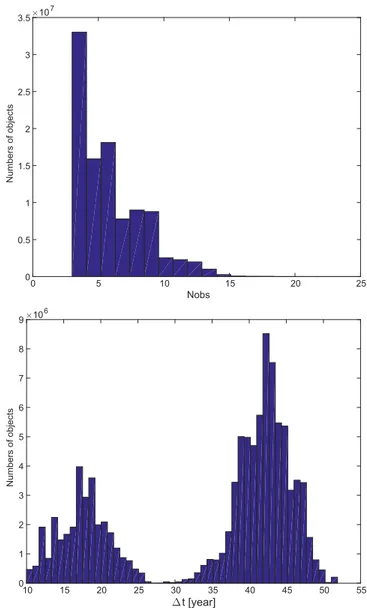
repeated observations of the samefields occur around the same time of the year. Properties(ii) and (iii) are well illustrated in Figures(2) and (3): the upper panel in Figure2shows that most of the APOP entries have only three measurements with less than 10% receiving 10 or more; Figure 3, providing the distribution of the folded observing times(folded to the fraction of the year on each observation was taken), clearly reveals a very uneven sampling, unsuitable for properly tracing the parallax ellipse. Actually, the lack of data points in a large interval, ∼0.35 years, around 0.5 years suggests that parallax induced positional changes are naturally minimized in our data as parallax factor differences tend to be small.

From Section 2, the precision of our best measurements is σx ∼ 0.15 arcsec; therefore, dividing this value by the

square root of the number of measurements, Nobs, yields a rough estimate of sensitivity to actual parallax shifts. By setting, Nobs = 10, although this actually happens for a very small fraction of the cases (Figure 2), we estimate (sp~sx Nobs ~ 0.050 arcsec), i.e., in the best case scenario, parallax would have a chance to show in our data (i.e., as nonlinear effects) but only for distances up to ∼20 pc. If we now consider again properties (ii), and especially (iii), from above, it becomes clear that parallax direct estimability

Figure 2. Distribution of the number of measurements per proper motion entry (top); distribution of epoch differences for the proper motions in APOP (bottom).

with our data is unlikely. Under these circumstances forcing a parallactic term in Equation (1) is likely to correlate parallax with proper motion itself, therefore justifying our decision to drop the parallax factors from the adopted reduction model. Yet we still need to address here the possible effects on the APOP proper motions of the parallax term we left unaccounted.

To this end, as recalled in Section 2, pairing plate measurements together (object matching) was done via the GSC2.3 object IDs (no actual re-matching of plate entries); therefore, APOP inherited the same 4 arcsec max matching radius utilized for the construction of the GSC2.3 (Lasker et al.2008). We anticipate here the characteristics of the proper motions we decided to export to the APOP catalog: each proper motion entry was generated after(1) fitting at least three plate measurements, and(2) rejecting fits with total epoch separation of less than 10 years(see lower panel of Figure 2).

At 20 pc a full parallax shift would show in our results, because of the 10-year condition (No.2) above, as a proper motion bias of ∼0.005 arcsec yr−1. At this distance even disk population stars exhibit proper motions of the order of 0.1 arcsec yr−1, for a bias-to-proper-motion ratio of only 5%. With local thick disk and halo stars moving at much higher spatial velocities(up to 10–20 times larger), this bias-to-proper-motion ratio drops to below 1% and 0.3%, for thick disk and halo stars, respectively. As both parallax and proper motion decrease with distance, this ratio could be seen as a value characterizing the quality of the APOP proper motions of the different Galactic populations independent of distance.

In conclusion, the considerations above provide evidence that the proper motion reduction model presented in the previous section is quite robust against parallax effects.

Finally, we still need to address here the effect of the 4 arcsec matching radius recalled before. Actually, for high proper motion samples (roughly higher than 0.4 arcsec yr−1 if below −30° decl., and 0.1 arcsec yr−1_{if above; see the lower panel of}

Figure2) involving Galaxy populations like WD and RD stars, this spatialfilter can cause the loss of those measurements with the largest epoch differences and therefore may not be the most useful for the best proper motion accuracy. Potential users in need of studying the properties of these important, but relatively small, high proper motion samples will have to decide if the APOP provided values are adequate for their applications.

3.2. Accurate Orientation to the Equatorial System The overall procedure just discussed only removes the systematic errors between reference and program plates; it can not remove the systematics inherent to the differences between plate-based coordinates and the standard coordinates.

This last registration is obtained using an external reference catalog and an account of the procedure follows.

We use a gnomonic projection to transform the estimated measured coordinates to an equatorial system. Since the Schmidt design provides an equidistant projection, we correct the measured coordinates following Dick (1991):

x x x x y y y y x y 1 3 1 3 , 8 G G 0 0 02 0 2 0 0 0 2 0 2

(

)

(

)

where xG, yG are the measured coordinates in a gnomonic

projection. By differentiating Equation(8) as a function of time

wefind the corresponding relations for proper motions:

x y x y y x x y 1 1 3 2 3 1 1 3 2 3 , 9 x x y y y x 0 2 0 2 0 0 0 2 0 2 0 0 G G ( ) m m m m m m = + + + = + + + ⎜ ⎟ ⎜ ⎟ ⎧ ⎨ ⎪⎪ ⎩ ⎪ ⎪ ⎛ ⎝ ⎞⎠ ⎛ ⎝ ⎞ ⎠ where _x G m , _y G

m are the proper motions in a gnomonic projection.

The transformation between the measured coordinates xG, yG

and their celestial standard coordinateξ, η can be expressed as

ax by c x y a x b y c x y , , , 10 G G G G G G G G ( ) ( ) ( ) x e h e = + + + = ¢ + ¢ + ¢ + ¢ ⎧ ⎨ ⎩

where a b c a b c, , , ¢ ¢ ¢ are the coefficients of the linear terms, , of the plate model, i.e., axis direction, scale and origin difference between the measured and standard coordinate systems; e(xG,yG) and e¢(xG,yG) represent the higher order

terms.

If we differentiate Equation(10) with respect to time, we get the proper motions in the standard coordinate system.

a b a b , 11 x y x y G G G G ( ) m m m m m m = + = ¢ + ¢ x h ⎪ ⎪ ⎧ ⎨ ⎩

where we have neglected higher order terms, which we estimate to be less than 0.03% of theμx,μy.

For the objects on the plate, there is a precise geometrical relationship between the standard coordinates and equatorial coordinates i.e.,

tan

cos sin

tan cos sin

cos sin cos

, 12 0 0 0 0 0 0 0 0 ( ) ( ) ( ) ( ) a a x d h d d h d d d h d a a - = -= + - -⎧ ⎨ ⎪⎪ ⎩ ⎪ ⎪

whereα0,δ0are the equatorial coordinates of the tangent point.

Finally, the rigorous relationship between proper motions in the equatorial and standard systems is obtained by differentiat-ing Equation(12) as a function of time, i.e.,

cos 1 cos sin sin cos sin cos cos cos cos sin

cos cos sin sin

cos sin

cos sin sin

cos sin . 13 2 0 0 0 0 0 0 2 2 0 0 0 0 0 0 0 0 0 0 2 0 0 0 0 0

(

)

(

)

(

)

(

)

3.3. Processing Pipeline

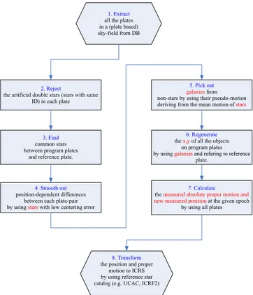
We developed a FORTRAN pipeline based on the above principles to determine absolute proper motions from the COMPASS database. Theflowchart (Figure4) summarizes the specific steps and techniques used to remove the systematic errors and to acquire the absolute proper motions. Key steps in theflow chart are detailed below.

In Steps 1–3 we extract all matches on the plates overlapping with the reference plate. Only objects that appear in all plates are used to calibrate the fit to the reference plate system.

In Step 4, a moving-mean-like method is applied to remove the mean shift(PdE and the mean proper motions of reference stars) in x and y between the program and reference plate. Only stellar objects are used in the calculation of the moving mean but the result is applied to all detections. In order to attain the most accurate coordinate transformation, we select reference stars with good image quality(i.e., with low centering errors, see Section 3.1). In particular, we use detections classified as star in the range m( lim-4.5)m(mlim-2.0), where mlim is the limiting magnitude of the plate, ∼20.5 in RF. In general

wefind around 500 stars degree−2well distributed on the plate. There are several methods for removing the PdE, such as a global plate solution using high-order polynomials, the astrometric MASK (Taff et al. 1990; Lattanzi & Bucciar-elli 1991), the Infinitely Overlapping Circles (IOC, Taff et al. 1992), the sub-plate method (Taff 1989) etc. All these methods have pros and cons: the Schmidt plate distortions would require very complicated global solutions, the MASK method is very sensitive to the number of reference objects and the grid size, the IOC has problems at the plate boundaries and the sub-plate method can lead to non-uniformities.

We developed a variant of the sub-plate method, the moving sub-plate method, that is sensitive to local signals while

ensuring an increased level of uniformity. The moving sub-plate method starts by transforming the measured coordinates x2, y2on the program plates to the corresponding coordinates

x1, y1 on the reference plate using cubic polynomials

(Equation (14)). This will remove most of the large-scale errors(e.g., spherical deformation).

x f x y y g x y , , , 14 1 2 2 1 2 2 ( ) ( ) ( ) = = ⎧ ⎨ ⎩

where the functions f and g are complete cubic polynomials. The residuals Δx, Δy, from the global (whole plate) cubic polynomialfit are then used in the following linear relations:

x ax by c y a x b y c, 15 2 2 2 2 ( ) D = + + D = ¢ + ¢ + ¢ ⎧ ⎨ ⎩

where a, b, c, a′, b′, c′ allow for zero point, rotation, and scale difference at a local level.

Tofit Equation (15) we select nearby reference stars within a radius of 20 arcmin from the program object. If more then 15 stars were found, they were ranked with distance from the program star and thefirst 15 were used for the fit; with less then 3 reference stars no correction was computed. Therefore depending on actual star density, the effective radius of a moving sub-plate can be much smaller then 20 arcmin. Applying this correction to all program objects removes most of the small scale errors(See Figure5). After Step 4, the mean displacement due to proper motion of the reference objects is locally zero, while that of galaxies is not.

In Step 5 we use Equation(16) on all the non-stars to fit a linear (coordinate only) model to estimate the mean proper motion components for any given plate pair, i.e., the- D inm¯_x t

Equation(5), and its analog for the y direction.

x x x ax by c y y y a x b y c, 16 1 2 2 2 1 2 2 2 ( ) D = - = + + D = - = ¢ + ¢ + ¢ ⎧ ⎨ ⎩

where x2, y2are intended as the measured coordinates of

non-stars on the program plate corrected for the systematics calculated in Step 4. As per Equation(5), we iterate rejecting any objects with residuals greater than 2.6 standard deviations9 per coordinate.

The objects that survive this selection are likely to be, or act like(i.e., non-stellar objects with zero proper motions), genuine galaxies. Figure6shows thefinal mean (pseudo) proper motion of the galaxies after completing Step 5 for the same plate pair as that of Figure5.

In Step 6 once the galaxies positions are corrected using the fitted coefficients of Equation (16), a two-dimensional map of the galaxies residuals shows that some PdE are still present. These are smoothed out using again the moving sub-plate method but this time using the selected galaxies as reference objects. The residual corrections found at this stage are applied to all of the objects. The subset of these values relative to the galaxies is then spatially binned and plotted against magnitude and color to seek for any remaining MdE and/or CdE signals.

Figure 4. Flowchart of the processing pipeline.

9 _{We found that the 2.6σ value (i.e., 99.0% probability of being within the} acceptable standard deviation) was optimal: a larger value provided many more objects to use with Equation(16) but larger fit errors (because of the inclusion of larger fraction of spurious galaxies, usually unresolved binaries or defects); on the other hand, a smaller threshold meant loosing too many good candidates for thefit.

In case, these are treated by simple one-dimensional linear interpolation in between the magnitude or color bins. This procedure removes most of the MdE and CdE between program and reference plates.

At this step we apply the mean motion to the stellar objects and remove it from the galaxies. From Figures7 to8we note that both MdE and CdE were significantly reduced.

In Step 7 for all of the plate objects we fit Equation (7) to determine absolute proper motions and positions at the given epoch J2000.0. We then correct the measured coordinates and

absolute proper motions derived in an equidistant projection to a gnomonic projection by using Equations(8) and (9).

In Step 8 we use the Fourth US Naval Observatory CCD Astrograph Catalog (UCAC4, Zacharias et al. 2013) and Equations (10)–(13) to transfer absolute proper motions and positions to the celestial reference frame. Moreover, we corrected the frame bias between APOP and the International Celestial Reference System (ICRS) by using 1288 objects (most of them are faint Quasi-stellar objects; QSOs) common to the radio ICRF2 catalog(Ma et al. 2009). To establish the

Figure 5. Upper figure shows the PdE as a function of plate position after the cubic polynomialsfitting. The vector represents the magnitude and direction of the average residual for the reference stars in that region of the plate. The data shown here come from the plate XP715 (epoch = 1996.3, l = 266 9, b= 69 2) and XE494 (epoch = 1955.3). The lower figure shows the same data as the one above after applying the moving sub-plate method. No observable PdE remains after this step. The marker“×” symbols indicate there are no common stars in those plate regions.

Figure 6. Mean pseudo “proper motion” of galaxies as a function of plate position.

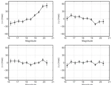
Figure 7. Mean residuals of the pseudo “proper motion” of the galaxies as a function of magnitude after Step 6. The upper two figures are the results without a magnitude term, while the lower panels are results with that term included. The magnitude is binned in 0.46 mag bins, with 300–2000 objects per bin for the different magnitudes.

orientation to the standard frame, we use the following formula r r r R R R 1 1 1 17 Y y X x Z z z y z x y x ICRF2 APOP APOP

( )

( )

( )

where rICRF2and rAPOPare the direction vectors to the common objects in both ICRF2 and APOP, respectively;ξx,ξy,ξzare the

three small rotation angles needed to register the APOP coordinate frame about the x, y and z axes of the ICRF2. A least-squares fit to Equation (17) provides estimates of those three angles:ξz= 27.73 ± 0.12 mas, ξx= −7.30 ± 0.15 mas,

andξy= 2.21 ± 0.06 mas; these are used to bring APOP onto

ICRF2. The ξx and ξy values are similar to those found in

Zacharias & Zacharias(2014), while the ξzrotation difference

is considerably large (ξz = 7.61 ± 1.21 in Zacharias’ work).

The actual cause is not clear at the moment but it could reside in the different samples used for the registration. After performing the transformation, the coordinate axes realized by our astrometric data are believed to be aligned, at least formally, with the extragalactic radio frame to within±0.2 mas at the reference epoch J2000.0.

4. CATALOG ACCURACY AND PRECISION We can estimate the accuracy and precision of our proper motions to provide us with a final external check. We expect the accuracy defined by the absolute zero point from Equation (16), assuming the observational errors are equally distributed among the fitted parameters, to be approximately given by t N 6 , 18 zero g g ∣ ∣ ( ) s = s D

whereσgis the positional measuring error of galaxies, 6 is the

number of unknown parameters andΔt is the epoch difference between two plates. This empirical error estimate has been confirmed by examining the formal error using simulated data. The range of positional measuring error of galaxies is in the range 0 2< σg< 0 5 for objects brighter than RF= 20.0, the

time baseline range is12< D <∣ t∣ 45years and the number of galaxies is 8000 < Ng < 20000. This corresponds to a

zero-point(absolutization) error of 0.1 < σzero< 1.1 mas yr−1.

If we assume the observations are evenly distributed about the mid-epoch we find that the formal error of each proper motion component from Equation(7) is

t N , 19 s obs ∣ ∣ ( ) s = s D m

where σs is the positional error, Nobs is the number of

observations of a star andá D ñ is the average time difference∣ t∣ between the various observations and the mid-epoch. The range of positional measuring error is ∼0 2 < σg< 0 3 for stars

brighter than RF = 20.0, the number of observations

3 < Nobs < 15, and the average time differences

t

12< D <∣ ∣ 45years. This corresponds to a range of overall error of 1< σ_μ< 14 mas yr−1.

We reduced all the plates with b∣ ∣ 27 and carried out an error analysis to certify the reliability of the calibration software and the quality of the final catalog, as described in the next sections.

4.1. Internal Precision

For each object, we calculated positions and proper motions byfitting Equation (7) utilizing all of the measurements from the different epochs and colors. This provides the formal errors of the calibrated parameters(μ_α*= μ_α× cos(δ), μ_δ,α, δ), and an internal check of the APOP quality.

In Figure9we plot the mean formal errors andfind them to be consistent in both R.A. and decl. even though the two

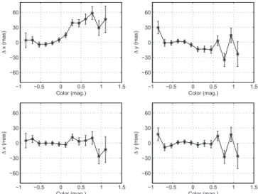
Figure 8. Same residuals as Figure7, but as a function of color. The upper two figures are the results without a color term, while the lower panels are results with that term included. The color, BJ− RF, is binned in 0.16 mag bins, with 60–2000 objects per bin as a function of color. The plots clearly show that the systematic corrections become statistically ineffective for colors larger than ∼0.5 in Δy due to small number of objects.

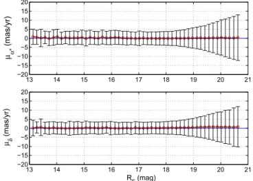
Figure 9. Mean formal errors of APOP absolute proper motions (μα*, μδ) and positions(α, δ) of stars and non-stars as a function of RF magnitude. The magnitude is binned in 0.3 mag bins, with at least 100,000 objects per bin. The marker*in theμαindicates multiplication by cos(δ). Top: the formal errors of absolute proper motions in mas yr−1; bottom: the formal errors of positions in mas.

coordinates were treated independently. For stellar objects, the internal accuracy of the proper motions is better than ±4 mas yr−1 _{for objects brighter than R}

F = 18.5, increasing

to 9 mas yr−1at RF= 20.0 and to 14 mas yr−1for objects with

20.0< RF< 20.8. The internal accuracy of the stellar positions

is better than ±100 mas for objects brighter than RF= 18.5,

increasing to 260 mas for objects with magnitude RF∼ 20.8.

The offset between the star and non-star objects is consistent with the ∼1.5 times larger measurement errors of non-stellar objects.

We note that objects close to the magnitude limit (i.e., 20 < RF < 21) have larger errors than predicted; APOP

parameters and errors should be used with caution for objects fainter than RF= 20.

An internal check of the accuracy of APOP proper motions is provided by multiple estimates for the same stellar objects appearing in overlap regions between adjacent reference plates. In Figure 10 we display the mean offset between the proper motions calibrated on two adjacent reference plates. The differences are plotted based on the position in the central reference XP216(l = 151 4, b = 62 8), which has a typical 1 5 × 6 5 overlap with four adjacent plates XP215 (left), XP217(right), XP170 (top) and XP266 (bottom). There are no large scale offsets in the overlap regions, but some shifts of ∼1.8 mas yr−1_{appear at small scales, particularly at the bottom}

left of the central plate. These are very likely caused by the uncertainty in the correction of the absolute zero point by the galaxies.

4.2. External Accuracy

QSOs have star-like images and since they are extragalactic, they do not exhibit any time-dependent displacement. Thus, we can use the mean and dispersion of their measured motions to

evaluate the zero point and overall precision of stellar proper motions. Here we use QSOs as an independent and direct determination of the APOP catalog quality.

The Gaia Initial QSO Catalog(GIQC; Andrei et al.2009) is chosen as the source list for known QSOs. The objects are broadly distributed within the SDSS region, though their density is not uniform(see Figure 11). Figures 12 –14 show the mean proper motions of the GIQC QSOs and indicate that there is a very good agreement between the external and theoretical error estimates of proper motions for the magnitude range RF< 20.5. In particular, from this sample of QSOs we

find a proper motion zero point error of 0.6 mas yr−1_{. As a}

verification of the internal estimates, Figure 15 shows the formal errors of positions (α, δ) of QSOs as a function of magnitude, and indicate that they are consistent with stellar objects.

In addition to the GIQC, we also compared APOP with other external catalogs. The most natural comparison would be with the Positions and Proper Motion XL catalog(herafter PPMXL, Roeser et al.2010) the largest most recent catalog with absolute proper motions. This was constructed by combining USNO-B1.0 and the Two Micron All Sky Survey (Skrutskie

Figure 10. Differences of proper motions (Δμα_{*, Δμ}δ) of common objects in the reference plate XP216 and overlapping plates as a function of position. The “Z” indicates the magnitude and direction of the differences of the average proper motions. A 5 mas yr−1scale arrow is plotted at the top left corner. The size of each bin is 0.25× 0.25 degree2_{and they contain on average 300 objects} per bin. The marker“×” indicates no objects in common, while a “◦” indicates that the number of the common objects is less than 100.

Figure 11. Density distribution of 376,490 QSOs found in the APOP catalog via cross-matching with the GIQC catalog.

Figure 12. Distribution of absolute proper motions (μα_{*, μ}δ) of QSOs as a function of magnitude. The red circles indicate the mean ofμα_{* and μ}δin that magnitude bin and the error bar shows their standard deviation, which, following the assumption that QSO should have zero proper motions, are indicative of the proper motion random errors. Thefigure clearly shows a ∼0.6 mas yr−1_{systematic offset in decl. proper motions for QSOs fainter then} 18 mag.

et al.2006) catalogs. Figures16and17illustrate that there is a systematic offset between these two catalogs in absolute proper motions.

We also selected a subset of the GIQC QSOs that were in both the APOP and the PPMXL for a comparison. Figure18 shows that the offset between the two catalogs is mostly due to a zero point problem in the PPMXL. Also, for most of the

Figure 13. The absolute proper motions found for the QSOs as a function of color.

Figure 14. Absolute proper motions found for the QSOs as a function of α and δ. As evidenced here, absolute proper motions data around the Large Magellanic Cloud region (center at αo = 80 9, δo = −69 7, apparent dimension is 10 8× 9 2) are not reliable and could cause an offset in μδ.

Figure 15. Formal errors of the QSO positions as a function of magnitude. The red circles indicate the mean formal errors ofα*andδ in that magnitude bin and the error bar shows their standard deviation. The magnitude is binned in 0.4 mag bins, with 38–21,539 objects per bin as a function magnitude.

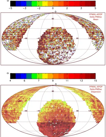
Figure 16. Mean (top figure) and dispersion (bottom figure) of differences in μδbetween APOP and PPMXL as a function of sky location in an equatorial coordinate system. The differences inμα_{* are quite similar. These plots are} based on the 82,722,482 common objects between these two catalogs divided in HEALPix(Hierarchical, Equal Area, and iso-latitude Pixelisation) level six regions.

Figure 17. Mean and dispersion (rms) of the proper motion differences between APOP and PPMXL as a function of magnitude.

magnitude range the APOP has smaller proper motion dispersion.

4.3. Galactic Clusters in APOP

Since the field of view of the Schmidt plate is very large (6.5 × 6.5 sq. deg) the mean proper motion of stellar objects could vary across the plate. For example, clusters generally cover a significant part of a photographic plate. Using the stars in Step 4 to remove the PdE we risk also“removing” the proper motions for this group of objects. Theoretically, we believe our procedure returns the mean proper motions to those groups with Steps 5 and 6. The proper motions of the Praesepe cluster in Figure19indicate that at least for this cluster the procedure has worked.

4.4. The Final Catalog

The catalog is available at Strasbourg’s astronomical Data Center (http://cds.u-strasbg.fr, catalog I/331); the description of the catalog data is detailed in Table1. In particular, APOP derived positions and proper motions are at epoch J2000.0 and on the ICRS-defined equator.

Given the evidence provided, we believe that APOP’s proper motions are reliable for operational applications as well as astrophysical research. However, the potential users should remember the following.

1. The accuracy is best for objects withδ … −30° because of the 45-year epoch difference between first and second generation survey plates; at lower declinations the quality can be about four times worse than that due to a time base of only 12 years.

2. Our data around the Large Magellanic Cloud region (center at αo = 80 9, δo= −69 7 and 10 8 × 9 2 in

size) are not entirely reliable, as the region is too crowded, which caused object detection to generate many spurious objects.

3. The accuracy may not be sufficiently good for objects with magnitude RF< 15.0 due to a lack of bright galaxies

on some plates and decreasing measuring precision due to heavier saturation effects. At this bright end, users should at least compare APOP’s values to those listed in bright

absolute catalogs like, e.g., UCAC4 (Zacharias et al.2013).

4. As explained in Section 3.1.1, when used in accurate work, especially with high proper motion stars, APOP values should be taken with caution because of possible residual parallax effects.

The items above provide users with the proper information to decide if the APOP entries are adequate for their applications.

5. CONCLUSIONS AND FUTURE WORK The main results from our study are the following.

1. The principles and techniques suitable for the derivation of absolute proper motions from survey plates, including the treatment for position, magnitude and color systema-tics are described.

2. The realization of the APOP catalog is presented. Because of the direct use of extragalactic objects, the catalog sky coverage is limited to the regions outside the galactic plane( b∣ ∣ 27).

The internal and external accuracies of this new catalog are consistent with expectations. The overall accuracy of the absolute proper motions is in the 3–9 mas yr−1 range, with an absolute zero point error estimated at better than 0.6 mas yr−1; this proves the feasibility and reliability of the principles and methods adopted for its construction. The average position accuracy is about 150 mas (per coordinate), with a systematic deviation from the ICRS around 0.2 mas. 3. A new method to refine source classification and select

bona fide galaxies by implementing the concept of induced pseudo-motion is presented.

Figure 18. Mean and dispersion of the absolute proper motions of the 360,127 QSOs common to both the APOP and the PPMXL as a function of magnitude.

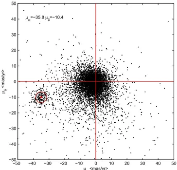
Figure 19. Proper motion vector-point diagram for all the objects in APOP with magnitude RF< 18.0 in the area of the Praesepe cluster. A tight group at μα_{* = −35.8 mas yr}−1, μδ = −10.4 mas yr−1 indicates the location of Praesepe and permits a segregation between the cluster and field stars. In addition, this value is quite close to the Hipparcos data for Praesepe, which is μα* = −35.81 mas yr−1,μδ= −12.85 mas yr−1(van Leeuwen2009).

We intend to apply a variant of this procedure to the whole GSC-II database to produce the GSC2.4. Some of the methods in this paper are only applicable in regions with significant numbers of extragalactic objects; therefore, we are working on new procedures for the galactic plane. Another residual source for concern is the offset between the magnitude systems of stars and galaxies(Lasker et al.2008). This reduces the effectiveness of removing the magnitude and color systematic errors by using galaxies.

Further investigations will clarify these issues as we prepare to extend APOP to the all sky with the production of GSC2.4.

This work is a joint study of the Shanghai Astronomical Observatory (SHAO), the Osservatorio Astrofisico di Torino (OATo) and the Space Telescope Science Institute (STScI). We would like to express our thanks to many former and present members of the GSC project for their support and effort for this large project. The STScI is operated by the Association of Universities for Research in Astronomy, for the National Aeronautics and Space Administration under contract NAS5-26555. This work is supported by grants from the National Science Foundation of China (NSFC No. 11273003, 10903022), the IPERCOOL FP7 International Research Staff Exchange Scheme(No. 247593), and the Italian Space Agency through contracts I/037/08/0 and I/058/10/0 (“The Italian Participation in the Gaia Mission”). M.G.L. acknowledges support from the Chinese Academy of Science through 2015 CAS President’s International Fellowship Initiative (PIFI) for Visiting Scientists.

This research has made use of the MCS database server system, developed by Giorgio Calderone and Luciano Nicastro, operated at OATo and SHAO. Finally, we wish to thank the people who gave us their suggestions and assistance throughout the realization of APOP, and especially Ming Zhao, William F. van Altena, Ramachrisna Teixeira, Nadia Maigurova, Alex-andre H. Andrei, Ronald Drimmel, Leigh Smith, Zhengyi Shao and Zi Zhu.

The anonymous Referee is thanked for suggestions and comments that significantly improved the initial version of this article.

REFERENCES

Andrei, A. H., Souchay, J., Zacharias, N., et al. 2009,A&A,505, 385 Curir, A., Lattanzi, M. G., Spagna, A., et al. 2012,A&A,545, A133 Curir, A., Serra, A. L., Spagna, A., et al. 2014,ApJL,784, L24 Dick, W. R. 1991,AN,312, 113

Evans, D. W., & Irwin, M. 1995,MNRAS,277, 820

Kallivayalil, N., van der Marel, R. P., Besla, G., Anderson, J., & Alcock, C. 2013,ApJ,764, 161

Kuimov, K. V. D. S. F., Kuz’Min, A. V., & Barusheva, N. T. 2000,ARep, 44, 474

Lasker, B. M., Greene, G. R., Lattanzi, M. J., McLean, B. J., & Volpicelli, A. 1998, in Astrophysics and Algorithms

Lasker, B. M., Lattanzi, M. G., McLean, B. J., et al. 2008,AJ,136, 735 Lasker, B. M., Sturch, C. R., McLean, B. J., et al. 1990,AJ,99, 2019 Lattanzi, M. G. 2012, MmSAI,83, 1033

Lattanzi, M. G., & Bucciarelli, B. 1991, A&A,250, 565 Ma, C., Arias, E. F., Bianco, G., et al. 2009, ITN,35, 1 Mahmud, N., & Anderson, J. 2008,PASP,120, 907

Morrison, J. E., Smart, R. L., & Taff, L. G. 1998,MNRAS,296, 66 Pryor, C., Piatek, S., & Olszewski, E. W. 2015,AJ,149, 42 Roeser, S., Demleitner, M., & Schilbach, E. 2010,AJ,139, 2440 Skrutskie, M. F., Cutri, R. M., Stiening, R., et al. 2006,AJ,131, 1163 Spagna, A., Lattanzi, M. G., Lasker, B. M., et al. 1996, A&A,311, 758 Spagna, A., Lattanzi, M. G., McLean, B., et al. 2004, MSAIt Supplement,5, 97 Spagna, A., Lattanzi, M. G., Re Fiorentin, P., & Smart, R. L. 2010,A&A,

510, L4

Taff, L. G. 1989,AJ,98, 1912

Taff, L. G., Bucciarelli, B., & Lattanzi, M. G. 1992,ApJ,392, 746 Taff, L. G., Lattanzi, M. G., Bucciarelli, B., et al. 1990,ApJL,353, L45 Tang, Z. H., Qi, Z. X., Yu, Y., et al. 2008, in IAU Symp., 248, A Giant Step:

from Milli-to Micro-arcsecond Astrometry, ed. W. J. Jin, I. Platais & M. A. C. Perryman(Cambridge: Cambridge Univ. Press), 334

van Altena, W. F., Girard, T., Lopez, C. E., Lopez, J. A., & Molina, E. 1990, in IAU Symp. 141, Inertial Coordinate System on the Sky, ed. J. H. Lieske & V. K. Abalakin(Cambridge: Cambridge Univ. Press),419

van Leeuwen, F. 2009,A&A,497, 209

Zacharias, N., Finch, C. T., Girard, T. M., et al. 2013,AJ,145, 44 Zacharias, N., & Zacharias, M. I. 2014,AJ,147, 95

Table 1

Description of the APOP Data Table Number Type Units Label Explanations 1 Char null ID source identifiera

2 Int null Type Classificationb

3 Double degree RA αICRS, J2000.0 4 Double degree DE δICRS, J2000.0

5 Float mas sigRA Error inα

6 Float mas sigDE Error inδ

7 Float mas/year PR μαcos(δ)

8 Float mas/year PD μδ

9 Float mas/year sigPR Error inμαcos(δ) 10 Float mas/year sigPD Error inμδ

11 Int null Nobs Number of observationsc 12 Float year Dt Maximal time differencesd 13 Float mag Rmag RFphotographic magnitude

e

14 Float mag Bmag BJphotographic magnitude 15 Float mag Nmag INphotographic magnitude 16 Float mag Vmag V photographic magnitude 17 Float mag Jmag 2MASS J magnitudef

18 Float mag Hmag 2MASS H magnitude

19 Float mag Kmag 2MASS Ksmagnitude Notes.

a

The ID is the source identifier for an object in the APOP, which is as same as the source identifier of that object in GSC2.3 catalog.bThe classification is based on the following codes: (0): Star as defined in the GSC2.3. (1): Stars used as reference objects.(2): QSOs from the GIQC catalog. (3): Non-stars as defined in the GSC2.3. (4): Non-stars indicated as extragalactic objects from Section3.2Step 5.cThe Nobs is the number of plates used for deriving theμα, μδof that object.dThe Dt is the maximal time differences between the plates used for the calculation.eThe magnitude data are extracted directly from the GSC2.3 catalog. Users can identify the exact meaning by looking at“Table 3” in GSC2.3 paper (Lasker et al.2008).fThe photometric data are the near-infrared J(1.25 μm), H (1.65 μm), and Ks(2.16 μm) from the 2MASS catalog (Skrutskie et al.2006).