Biomechanical analysis using the skeleton measured by the Microsoft Kinect V2

(1)

POLITECNICO DI MILANO

School of Industrial and Information Engineering

Master of Science in Mechanical Engineering

Biomechanical Analysis Using The Skeleton Measured By

The

Microsoft Kinect V2

Supervisor:

Ing. Marco TARABINI

Authors: Marco MARINONI 837808 Matteo MASCETTI 853977

(2)

(3)

5.4.2 CPDF Analysis ... 104 5.4.2.1 Operation 700 ... 106 5.4.2.1.1 Shoulder Angles ... 106 5.4.2.1.2 Elbow Angles ... 106 5.4.2.1.3 Wrist Angles ... 107 5.4.2.2 Operation 701 ... 107 5.4.2.2.1 Shoulder Angles ... 107 5.4.2.2.2 Elbow Angles ... 108 5.4.2.2.3 Wrist Angles ... 108 5.4.2.3 Operation 722 ... 109 5.4.2.3.1 Shoulder Angles ... 109 5.4.2.3.2 Elbow Angles ... 109 5.4.2.3.3 Wrist Angles ... 110

(5)

5.4.2.4 Operation 812 ... 110 5.4.2.4.1 Shoulder Angles ... 110 5.4.2.4.2 Elbow Angles ... 111 5.4.2.4.3 Wrist Angles ... 111 5.4.2.5 Operation 1310 ... 112 5.4.2.5.1 Shoulder Angles ... 112 5.4.2.5.2 Elbow Angles ... 112 5.4.2.5.3 Wrist Angles ... 113 5.4.2.6 Operation 1311 ... 113 5.4.2.6.1 Shoulder Angles ... 113 5.4.2.6.2 Elbow Angles ... 114 5.4.2.6.3 Wrist Angles ... 114 5.4.2.7 Operation C913 ... 115 5.4.2.7.1 Shoulder Angles ... 115 5.4.2.7.2 Elbow Angles ... 115 5.4.2.7.3 Wrist Angles ... 116

5.4.3 Influence of Time Over Kinect System ... 116

5.4.3.1 Time higher than 90% ... 116

5.4.3.2 Time between 70% and 90% ... 117

5.4.3.3 Time between 50% and 70% ... 119

5.4.3.4 Time Less than 50% ... 122

5.4.4 Tests Summary ... 126

5.5 Discussion ... 127

6 Conclusions ... 129

(6)

(7)

Table List

Table 1 – Main motion tracking systems (Zhou and Hu 2008) ... 3

Table 2 – Comparison between non-contact systems without markers ... 4

Table 3 – ToF cameras main characteristics ... 13

Table 4 – Resolution definitions ... 14

Table 5 – FrLim analysis ... 24

Table 6 – Regression analysis for # of frames / FrLim curve ... 25

Table 7 – Successful rate in percentage for tests combining the same subject for static and dynamic acquisitions, varying FrLim ... 30

Table 8 – Successful rate in percentage for tests combining different subjects for static and dynamic acquisitions, varying FrLim ... 30

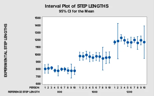
Table 9 – Mean and StDev of all tests obtained with former algorithms (all results in [mm]) ... 70

Table 10 – Mean and StDev of P01, P02 and P04 obtained with former algorithms (all results in [mm]) ... 71

Table 11 – Mean and StDev obtained with latest algorithms (all results in [mm])... 71

Table 12 – Comparison between former and latest algorithms (all results in [mm]) .. 71

Table 13 – Center of mass projection on ground results ... 92

Table 14 – Relative distance: Center of mass - ground results ... 93

Table 15 – Head acceleration method results ... 94

Table 16 – Torso inclination results... 95

Table 17 - Performed tests ... 99

Table 18 – Operations acceptable angles range ... 103

(8)

(9)

Figure List

Figure 1 – Tof Camera basic principle (Li 2014) ... 5

Figure 2 – RGB and depth map representation (Li 2014) ... 5

Figure 3 – Full TI Tof System , OPT8241 on the right ... 6

Figure 4 – EPC660 Card Edge Connector Carrier ... 7

Figure 5 – STM VL53L0X Sensor ... 7

Figure 6 – Kinect components ... 8

Figure 7 – Point Cloud provided by Kinect SDK ... 9

Figure 8 – CompleteViewer interface ... 10

Figure 9 – CompleteViewer subfolders ... 10

Figure 10 – Skeleton representation ...11

Figure 11 – Skeleton nodes joint ID map ...11

Figure 12 – Kinect reference system ... 12

Figure 13 – Objectives of the master thesis for the home environment ... 15

Figure 14 – Mode operandi at the end of thesis work (in green, areas relevant for the algorithms implemented) ... 16

Figure 15 – Mode of operation of the finished product... 16

Figure 16 – Master thesis objectives for work environment field ... 17

Figure 17 – Raw acquisition ... 19

Figure 18 – Focus on way in – way out distortions of the skeleton ... 19

Figure 19 – Reference skeleton from a static acquisition ... 20

Figure 20 – Scatterplot of acquired frames varying the value of FrLim ... 25

Figure 21 – Probability plot of standardized residuals ... 26

Figure 22 – Scatterplot of SRES vs FITS ... 26

Figure 23 – Tangent steepness reduction after minimum FrLim ... 27

Figure 24 – Windowed dynamic acquisition ... 28

Figure 25 – Focusing on upper body part ... 34

Figure 26 – Angles of interest for shoulder, elbow and wrist ... 35

Figure 27 – Schematic representation of the analysis by steps ... 36

Figure 28 – Schematization of the situation before and after data resampling... 37

Figure 29 – Skeleton in Kinect reference system ... 38

Figure 30 – Skeleton in ground reference system ... 39

Figure 31 – Functions scheme for skeleton representation in trajectory reference system ... 39

Figure 32 – Skeleton in trajectory reference system ... 40

Figure 33 – IdentifyFootStatus logic ... 41

Figure 34 – Histogram: Foot speed / number of occurrences ... 42

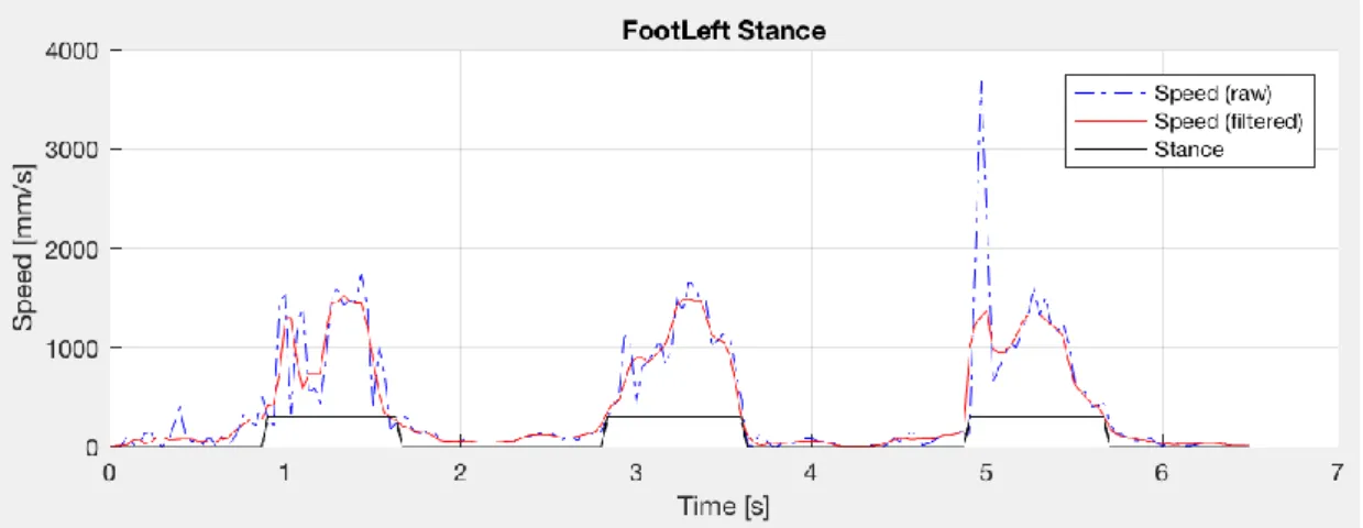
Figure 35 – Left foot information from IdentifyFootStatus ... 43

Figure 36 – Right foot status from IdentifyFootStatus ... 43

Figure 37 – Joint’s x, y, z coordinates in time ... 44

(10)

Figure 39 – Foot joint’s speed ... 45

Figure 40 – Left, right and total step lengths ... 46

Figure 41 – Left, right and total swing times ... 47

Figure 42 – Left, right and total stance times ... 47

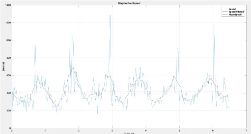
Figure 43 – Center of mass speed, filtered center of mass speed and center of mass mean speed ... 48

Figure 44 – Center of mass’s lateral oscillation ... 49

Figure 45 – Center of mass’s vertical oscillation ... 49

Figure 46 – No analysis (a): lack of upright configuration ... 50

Figure 47 – No analysis (b): lack of seated configuration ... 51

Figure 48 – Accepted acquisition ... 51

Figure 49 – Center of mass trajectory during a standing up in three dimensions ... 52

Figure 50 – Center of mass speed (spine base) in standing up phase ... 52

Figure 51 – Head speed in standing up phase ... 53

Figure 52 – Center of mass’s vertical displacement ... 53

Figure 53 – Center of mass’s lateral displacement... 54

Figure 54 – Part of interest of the acquisition ... 54

Figure 55 – Head vertical speed in raising movement ... 55

Figure 56 – Head vertical speed in descending movement ... 56

Figure 57 – Fall recognition in ground reference system ... 56

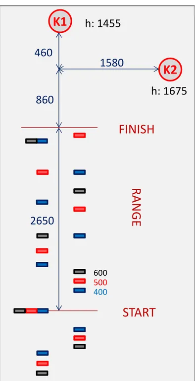
Figure 58 – Representation of the experiment setup for validation of the walk algorithm ... 60

Figure 59 – Experiment environment ... 61

Figure 60 – Particulars of the camera positioning ... 61

Figure 61 – Positioning of the toe on ground marker ... 62

Figure 62 – Skeletons acquired during one of the test ... 63

Figure 63 – Colored point cloud of the environment in Villa Beretta ... 64

Figure 64 – Left and right entrance walks setup ... 65

Figure 65 – RGB and Skeleton of static acquisition ... 66

Figure 66 – Environment point cloud showing paths... 66

Figure 67 – Left and right entrances Skeleton ... 67

Figure 68 – Foot status identification for left foot (P04, Session 1, 1200mm) ... 68

Figure 69 – Foot status identification for right foot (P04, Session 1, 1200mm) ... 68

Figure 70 – Example of cut step (P04, Session 2, 1000mm) ... 69

Figure 71 – Example of acquisition with an outlier of great amplitude ... 69

Figure 72 – Example of acquisition with high rumor (P02, Session 1, 1000mm) ... 69

Figure 73 – Interval Plot of Step Lengths for tests for the validation of walk algorithms ... 70

Figure 74 – Spine base oscillation in z for P02, tests for the validation of walk algorithm ... 72

Figure 75 – Spine base oscillation in z for P02, tests for the validation of walk algorithm ... 72

Figure 76 – Example of acquisition characterized by high rumor and a wrong foot status recognition, walk along a nonlinear trajectory test ... 73

(11)

Figure 77 – No step acquisition, walk along a nonlinear trajectory test ... 73

Figure 78 – One step, walk along a nonlinear trajectory test ... 74

Figure 79 – Two steps, walk along a nonlinear trajectory test... 74

Figure 80 – Joint oscillation in Z direction, Villa Beretta test ... 75

Figure 81 – Joint Oscillation in Y direction, Villa Beretta test ... 75

Figure 82 – Step lengths for P08, Villa Beretta tests... 76

Figure 83 - Swing times for P12, Villa Beretta tests ... 76

Figure 84 – Stance times for P08, Villa Beretta tests ... 77

Figure 85 – Step frequencies for P04, Villa Beretta tests ... 77

Figure 86 – Left and right sitting setup ... 79

Figure 87 – Sitting on armchair setup ... 79

Figure 88 – Environment point cloud showing sit procedure ... 80

Figure 89 – Skeletons acquired during sits ... 81

Figure 90 – Environment point cloud of last sitting procedure ... 82

Figure 91 – Skeletons acquired during sits on armchair ... 82

Figure 92 – Center of mass in descendent phase ... 83

Figure 93 – Center of mass in ascendant phase ... 84

Figure 94 – Head in descendant phase ... 84

Figure 95 – Head in ascendant phase ... 85

Figure 96 – Setup fall from chair ... 86

Figure 97 – Setup fall forward ... 87

Figure 98 – Setup fake fall, fall Lh ... 87

Figure 99 – Setup fake fall, fall Rh ... 88

Figure 100 – Setup floor sitting – raising ... 88

Figure 101 – Acquisition of a fall from chair ... 89

Figure 102 – Acquisition of a fall forward ... 89

Figure 103 – Acquisition of walk, fake fall and fall on left side ... 90

Figure 104 – Acquisition of Walk, fake fall and fall on right side ... 90

Figure 105 – Acquisition floor sitting/raising ... 91

Figure 106 – Simultaneous Radius-Distance magnitude during the fall ... 92

Figure 107 – Relative distance center of mass – ground during the fall ... 93

Figure 108 – Head position, velocity and acceleration in time during the test... 94

Figure 109 – Torso inclination in time during the test ... 95

Figure 110 – Notch system ... 97

Figure 111 Setup with 6 (Day A) and 7 (Day B) Notch ... 100

Figure 112 – Wearable system calibration ... 100

Figure 113 – Work Stations analyzed: a) 700 b) 701 c) 722 d) 812 e) 1310 f) 1311 g) C913 ... 101

Figure 114 – Setup for Kinect V2 on workstations ... 102

Figure 115 - Right elbow angle measured in ironing operation through the systems Kinect (red) and Notch (blue) vs Time ... 104

Figure 116 - Comparison between CPDF obtained through Kinect and Notch systems ... 105 Figure 117 –Right and Left shoulder Flex-Extension and Abduction-Adduction angles

(12)

for the operation 700 ... 106 Figure 118 – Right and left elbow Flex-Extension and Prono-Supination angles for the

operation 700 ... 106 Figure 119 – Left wrist Flex-Extension and Radial Ulnar angles of operation 700 . 107 Figure 120 – Right shoulder Flex-Extension and Abduction-Adduction and left

shoulder Flex-Extension angles for the operation 701 ... 107 Figure 121 – Right elbow Flex-Extension and Left elbow Flex-Extension and Prono-Supination angles for the operation 701 ... 108 Figure 122 – Left wrist Radial and Ulnar angle for the operation 701 ... 108 Figure 123 – Right shoulder angles of Flex-Extension and Abduction-Adduction and

left shoulder angles of Flex-Extension for the operation 722 ... 109 Figure 124 – Right and left elbow angles of Flex-Extension and Prono-Supination for

the operation 722 ... 109 Figure 125 – Right wrist angles of Flex-Extension and Left wrist Flex-Extension and

Radial Ulnar angles for the operation 722 ... 110 Figure 126 – Right shoulder angles of Flex-Extension and Abduction Adduction and

left shoulder angles of Flex-Extension for the operation 812 ... 110 Figure 127 – Right elbow angles of Extension and left elbow angles of Flex-Extension and Prono-Supination for the operation 812 ... 111 Figure 128 – Right and left wrist angles of Flex-Extension and Radial Ulnar for the

operation 812 ... 111 Figure 129 – Right and left shoulder angles of Flex-Extension and Abduction

Adduction for the operation 1310... 112 Figure 130 – Right and left elbow angles of Flex-Extension and Prono-Supination for

the operation 1310 ... 112 Figure 131 – Right wrist Flex-Extension and Radial Ulnar angles for the operation 1310 ... 113 Figure 132 – Right and left shoulder Flex-Extension and Abduction Adduction angles

for the operation 1311 ... 113 Figure 133 – Right and left elbow Flex-Extension and Prono-Supination angles for the

operation 1311 ... 114 Figure 134 – Right wrist Flex-Extension and Radial Ulnar angles for the operation 1311 ... 114 Figure 135 - Right shoulder Flex-Extension and Abduction Adduction angles and left

shoulder Flex-Extension angles for the operation C913 ... 115 Figure 136 - Right and left elbow Flex-Extension and Prono-Supination angles for the

operation C913 ... 115 Figure 137 - Right wrist Flex-Extension and Radial Ulnar angles for the operation C913 ... 116 Figure 138 – Left shoulder Flex-Extension angles comparison acquired by Notch and

Kinect systems (operation 701, test T13_17022017_163006) ... 116 Figure 139 - Right shoulder Abduction-Adduction angles comparison acquired by

Notch and Kinect systems (operation 701, test_701_T7) ... 117 Figure 140 – Left elbow Flex-Extension angles comparison acquired by Notch and

(13)

Kinect systems (operation 701, test_701_T6) ... 117 Figure 141 - Right shoulder Abduction-Adduction angles comparison acquired by

Notch and Kinect systems (operation 701, test_701_T6) ... 118 Figure 142 – Right elbow Flex-Extension angles comparison acquired by Notch and

Kinect systems (operation 1311, test_1311_T3) ... 118 Figure 143 – Left elbow Flex-Extension angles comparison acquired by Notch and

Kinect systems (operation 700, test T3_17022017_141512) ... 119 Figure 144 - Left shoulder Flex-Extension angles comparison acquired by Notch and

Kinect systems (operation 700, test T3_17022017_141512 ... 119 Figure 145 – Left elbow Flex-Extension angles comparison acquired by Notch and

Kinect systems (operation 700, test T1_17022017_135853) ... 120 Figure 146 - Left shoulder Flex-Extension angles comparison acquired by Notch and

Kinect systems (operation 700, test T1_17022017_135853) ... 120 Figure 147 - Right elbow Flex-Extension angles comparison acquired by Notch and

Kinect systems (operation 812, test_812_T3) ... 121 Figure 148 - Right elbow Flex-Extension angles comparison acquired by Notch and

Kinect (operation 700, test T3_17022017_141512) ... 122 Figure 149 - Right shoulder Flex-Extension angles comparison acquired by Notch and

Kinect systems (operation 700, test T3_17022017_141512) ... 122 Figure 150 - Right elbow Flex-Extension angles comparison acquired by Notch and

Kinect systems (operation 700, test T1_17022017_135853) ... 123 Figure 151 - Right shoulder Abduction-Adduction angles comparison acquired by

Notch and Kinect systems (operation 701, T1_17022017_135853) ... 123 Figure 152 - Left shoulder Flex-Extension angles comparison acquired by Notch and

Kinect systems (operation 722, test_722_T2) ... 124 Figure 153 - Right shoulder Abduction-Adduction and Flex-Extension angles

comparison acquired by Notch and Kinect systems (operation 1311, test_1311_T3) ... 125

(14)

(15)

Abstract. This thesis describes the algorithms implemented to perform biomechanical

analyses starting from the skeleton acquired by the Microsoft Kinect V2 Time-of-Flight (TOF) camera. The first set of algorithms were developed in order to analyse common daily life operations such as the gait, sitting/standing up and identifying people laying on the ground. Algorithms were implemented by analysing preliminary tests performed in controlled (laboratory) conditions. Their effectiveness in the identification of the gait and daily life parameters was then verified in different houses, rehabilitation structures and offices.

The second set of algorithms was developed in order to identify the range of motion of the upper limb. In this case, analyses were finalized at the computation of the OCRA index. Algorithms were used to estimate the biomechanical loads during sewing operations.

The validity of the proposed algorithms was proved by comparing the measures with those of gold standards. Results showed that the system is reliable in both controlled and real conditions whenever there are no occlusions between the 3D camera and the observed subjects. In order to overcome the limitations deriving from false skeleton recognitions in presence of occlusions, specific procedures for the validation of the measured skeleton were developed as well. Results evidenced that the system can be successfully used in dwellings for the recognition of the daily life activities and for gait analysis. The usage in industrial environment strongly depend on the chance of occlusions, that may limit the usability of the Kinect V2 in specific conditions.

Il presente lavoro di tesi descrive gli algoritmi implementati per effettuare analisi biomeccaniche partendo dallo skeleton misurato dal Kinect V2 di Microsoft. Un primo set di algoritmi è stato sviluppato per analizzare operazioni di vita quotidiana come la camminata, la seduta/alzata da una sedia e identificare persone sul pavimento in seguito a cadute. Gli algoritmi sono stati sviluppati analizzando delle prove effettuate in condizioni di laboratorio. La loro efficacia è stata verificata in condizioni operative presso uffici, strutture di riabilitazione e abitazioni private.

Un secondo gruppo di algoritmi è stato sviluppato per analizzare il moto degli arti superiori per il calcolo del carico biomeccanico secondo il protocollo OCRA.

Gli algoritmi sono stati validati in laboratorio confrontando i parametri con valori di riferimento acquisiti da altri sistemi di misura. I risultati hanno mostrato che, sia in condizioni di laboratorio sia in condizioni reali, il sistema è in grado di misurare correttamente la biomeccanica del moto qualora i giunti misurati dal kinect siano misurati e non stimati. In presenza di occlusioni, il sistema perde di efficacia; sono stati quindi sviluppati algoritmi specifici per censurare artefatti di misura generati dal Kinect stesso.

I risultati sperimentali hanno mostrato che il sistema può essere utilizzato con successo nelle abitazioni per monitorare gli spostamenti delle persone e per effettuare analisi del cammino. In ambiente industriale il sistema può essere usato a patto di non avere occlusioni rilevanti tra la camera e il soggetto.

(16)

(17)

1. Introduction

Human motion tracking is a field rapidly and continuously developing, embracing many areas, from movie making to video gaming, from sport to entertainment. The possibility to use the Kinect V2 Time of flight camera for healthcare and biomechanical load estimation is investigated.

A brief introduction to the classification of the human motion tracking systems is presented in chapter 1, with focus on non-contact ones. Besides, Time-of-Flight Cameras are described in their basic principle and in their components, as well as what market offers (in terms of sensor and cameras).

The algorithms implemented to analyse the biomechanics starting from the skeleton are presented in chapter 2. The main functions implemented are the censoring of the non-reliable parts of the acquisition (“windowing”) and the subject recognition from a database. Starting from the essential explanation of what the static and dynamic acquisitions are, the modus operandi of the two algorithms is presented.

In chapter 3, the parameters related to walking, sitting/standing up, falling and movements of the upper body part are fully described, as well as the algorithms implemented for their recognition.

Tests performed in dwellings and in work environment are presented in chapter 4 and 5 respectively. In these chapters, the experiments necessary to gather enough data to implement algorithms and to validate them are described, including their setup and execution. The thesis conclusions are drawn in section 6.

(18)

(19)

1 Human Motion Tracking Systems

Motion capture techniques are used over a large field of applications, from digital animation for entertainment to biomechanics analysis for clinical, rehabilitation and sport applications. Nowadays, it can be possible to find different body tracking systems on the market, with different performances, main applications and, obviously, costs. A tracking system can be non-visual based, visual based (marker based or markerless based), robot aided based or a combination of them (Zhou and Hu 2008), as reported in Table 1:

Table 1 – Main motion tracking systems (Zhou and Hu 2008)

The thesis work is completely based on the use of a visual based tracking system, that is also a non-contact type of measurement tool. The main non-contact systems without marker for 3D imaging are Time of Flight (ToF), Stereoscopic vision, Fixed structured

light and Programmable structured light. In Table 2, a comparison between the 3D

imaging technologies is presented, including application fields

(20)

Table 2 – Comparison between non-contact systems without markers

As it can be noticed, the main advantage for the Time-of-Flight cameras is the overall flexibility and easiness of use accompanied by good performances in many contexts. Thanks to these characteristics, they are applied in many fields. The following section is focused on the ToF cameras.

1.1 Time of Flight Cameras (ToF)

Time of Flight cameras (ToF cameras) provide 3D images of the entire scene through the calculation of speed of light, usually pulsed, coming from an integrated source. ToF cameras base their increasing success, since the early 2000s, on their simplicity, compactness, easy-of-use and high reliability of the images realized.

Nowadays, the market of ToF cameras is rapidly growing, even if the available and purchasable products remain few. Many of them use the same receiving sensors produced by Texas Instruments or ESPROS Photonics Corporation (EPC). There can be found, also, lot of prototypes reserved for developers or cameras no longer available or promoted but never born. In the following paragraphs, the working basic principle of ToF cameras is described; then a general description of the receiving sensor, a brief synthesis of the market supply and final considerations are proposed.

(21)

1.1.1 Basic Principles

Figure 1 – Tof Camera basic principle (Li 2014)

The basic principle of the Time of Flight cameras, as explained in the technical paper “Time-of-Flight Camera – An introduction” by Larry Li, is to illuminate the field of view through modulated light, receive the reflected rays by means of a matrix of photo-diodes and compute their traveling time (the so-called “time of flight”) analyzing the phase shift between illumination and reflection. Time of flight is then used to compute the distance of the point hit. This operation is conducted for the entire scene (differently from a “point-by-point” system) and in an acceptable fast way (about 30-150fps) for many applications.

All information is 3D represented in the so-called “point cloud”, one for each frame, collecting all the points tracked (named voxels) starting from their coordinates in a specific coordinate system. Otherwise, data can be represented in 2D in the “Depth

Map”. InFigure 2, a representation of the same field of view in RGB and depth map:

Figure 2 – RGB and depth map representation (Li 2014)

Point cloud looks like the depth map representation, but is possible to rotate it, moving in space.

(22)

ToF cameras are typically made by the following parts:

 Light Source: emits the light source needed, usually laser or NIR;  Electronic hardware: with control function;

 Optics: to correctly direct the outgoing light;  Sensor: receives the incoming light.

These components can be integrated in a little structure, measuring few centimeters, resulting light and easy to manage.

The future diffusion of ToF cameras probably lies in the large application to smartphones. A first model has presented in December 2016, the Lenovo Phab 2 Pro integrated with Google Tango Project.

1.1.2 Sensors

In this paragraph, a brief description of some of the most used in cameras ToF sensors.

Texas instruments (TI) – OPT8241

The OPT8241 time-of-flight (ToF) combines ToF sensing with an analog-to-digital converter (ADC) and a programmable timing generator (TG). The device offers quarter video graphics array (QVGA 320 x 240) resolution data at frame rates up to 150 frames

per second (600 readouts per second). In Figure 3, a schematic representation of the

whole system is given:

(23)

ESPROS Photonics Corporation (EPC) – Epc660

The epc660 is a 3D-TOF imager with a resolution of 320 x 240 pixels (QVGA). A resolution in the millimeter range for measurements up to 100 meters is feasible. 65 full frame TOF images are delivered in maximal configuration.

Figure 4 – EPC660 Card Edge Connector Carrier STMicroelectronics – VL53L0X

The VL53L0X is a Time-of-Flight (ToF) laser-ranging. It can measure absolute distances up to 2m. The render of the STMicroelectronics’ sensor is presented in Figure 5:

(24)

1.1.3 Microsoft Kinect One (V2) Full Specifications and Software

Microsoft Kinect V2 (2013) is a Time-of-Flight camera that substitutes the first version present on market (2010).

The device is composed by, referring toFigure 6:

 IR source obtained by the use of three lasers  Receiving depth sensor with 512x424 resolution  RGB camera with Full HD resolution

 4 Microphone

Figure 6 – Kinect components

The device is born for Xbox console with gaming purpose, but it is also available a Software Development Kit (SDK) for general application. To do so, a specific PC-adapter has been released. Kinect market spreading is based on the robustness of the results, its cheapness (99€, May 2017), easy-of-use and large diffusion of scientific documents.

The most important feature of the device related to this thesis is the presence of the depth camera which provides 512x424 pixel colour depth maps and point clouds. In

Figure 7,an example of point cloud provided by the Kinect SDK is represented. It could

be noticed: the conical fields of view of the camera (in the vertex), red cone where information is reliable and grey where is not, the identified ground and the Skeleton (illustrated in the following).

(25)

Figure 7 – Point Cloud provided by Kinect SDK

Software Development Kit permits to record all or part of the information deriving from the camera at a frame rate of 30 frames per second.

The tracking algorithm has memory of the previous frames, so the system has more difficulties in the static conditions respect to when skeleton is already acquired (Huber et al. 2015).

However, for thesis purpose, another software is mainly used: CompleteViewer-D2D

V2.0 (No-OpenCv) available for free at

http://www.tlc.dii.univpm.it/blog/databases4kinect. Using this software, it is possible to

(26)

The interface of the program is shown in Figure 8:

Figure 8 – CompleteViewer interface

CompleteViewer, after having concluded the acquisition, creates a folder with seven subfolders, as represented in Figure 9:

Figure 9 – CompleteViewer subfolders

Data collected are the following:

 Body: Excel file containing coordinate of the Skeleton of all frames recorded  Color: RGB images

 ColorPng: not relevant

 Depth: file .bin containing depth map  Infrared: not relevant

 Mapp: not relevant

(27)

RGB images acquisition is not relevant for the data elaboration, but it’s a good tool to verify what is happening in the scene for cross checking.

One of the most interesting peculiarity of the Kinect is the built-in recognition of the human body through the point cloud. The system identifies the so called “Skeleton” in real time, representing it by means of twenty-five “joints” their connections (Figure 10).

Figure 10 – Skeleton representation

Each joint is marked by a unique number: the map of the whole body is available in Figure 11:

(28)

The entire thesis bases its data elaboration on the use of the coordinates and time history of the Skeleton, implicating all its advantages and disadvantages. However, all the techniques and methods adopted and elaborated can be applied to any possible body reconstruction deriving from point clouds, that is with whichever ToF camera.

Microsoft Kinect V2 has its own coordinate system, available in Figure 12: Z axis “going out” from the lens; Y as vertical axis; X-axis measuring lateral displacement.

Figure 12 – Kinect reference system

Regarding the performance of the Kinect V2, less studies, respect to the first version of the ToF camera, are available (Giancola et al. 2015). Comparisons are made (Zennaro et al. 2015) and results shows that the second version is about twice more accurate in the near field of view and it increases in the farthest one. The robustness increases too, in terms of adaptation to the artificial light and the sunlight.

OpenPTrack, an open source software for multi-camera people tracking, has been studied in its performances (Munaro, Basso and Menegatti 2016). In a comparison with a wide range of 3D sensors, showing that Microsoft Kinect V2 is absolute the most

capable in people tracking.

1.1.4 Considerations

Time of flight sensors market supply is limited to few products, generally proposing similar performances in terms of resolution and frame rate. A trade-off exists between the two: the higher the resolution, the lower the frame rate. Usually, resolution QVGA 320 x 240 pixels is available when cameras work at 60 frames per second.

(29)

Table 3 – ToF cameras main characteristics Field of view (H x V x D) Resolution Range DS525 DepthSense Camera 74° x 58° x 87° (Depth) 63.2° x 49.3° x 75.2° (RGB) QVGA (Depth) HD (RGB) 0.15m – 1.0m LIPSedge DL 74° x 58° x 88° (Depth) 79° x 50° x 88° (RGB) VGA@30fps (Depth) FHD@30fps (RGB) 10cm – 8m ALL-TOF Type 67.1° x 54.6° x 41.4° VGA@45fps 0.3m – 9.6m ToF640-20gm_850nm 57° x 43° VGA 0m – 13m EKL3106 D-Imager 3D Image Sensor 60° x 44° nd 1.2m – 5m Taro ? 120 x 80 Up to 5m CamBoard pico flexx 62° x 45° 224 x 171 0.1m – 4m Xtion PRO LIVE 58° x 45° x 70° QVGA@60fps (Depth) VGA@30fps (Depth) SXGA (RGB) 0.8m – 3.5m Q60U-Series 70°x58°x45° (Depth) 74°x63°x49° (RGB) VGA@30fps (Depth) UVGA (RGB) 0.5m – 6m Starform nd nd 0m – 8m P321 90° (D) 160x120 0.1m – 3m

Persee 60° x 49.5° x 73° VGA (Depth)

WXGA (RGB) 0.4m-8m (optim. 0.6-6) BlasterX Senz3D 85° (D) (Depth) 77° (D) (RGB) VGA@60fps (Depth) Full HD@30fps (RGB) 0.2m – 1.5m Kinect V2 70° x 60° 512x424@30fps (Depth) Full HD@30fps (RGB) 0.4m – 4.5m

(30)

Table 4 – Resolution definitions Definition Resolution QVGA 320x240 VGA 640x480 WXGA 1280x720 HD 1360x768 SXGA 1280x1024 Full HD 1920x1080

ToF cameras are characterized by similar performances in terms of resolution and range. Specifically, VGA at 30 frames per second is the most common configuration and range varies between few tens of centimeters to 4 to 7 meters. Kinect V2 fits in these intervals, at a lower price respect to the average of the market supply.

1.2 Home Environment

The main idea of this work is to use one or more ToF cameras to track, characterize and analyse person’s indoor movements, mainly at home or in a medical centre, with interest for elderly people or in general for people needing assistance. Cameras are placed in adequate positions inside the space, in order to have reliable data over the time. Data collected could be employed in numerous way for the purposes of the healthcare. The effort is focused on three person states: walking, sitting and fall. First two are taken into consideration to have feedback about the health condition of the individual, the third is studied to implement an additional feature, the “fall-detection”. The data history of some crucial parameters, created over the time through non-consequential acquisitions, are meant to be analysed by medical staff. As an example, if the person of interest has an average step length of 1.20m, computed from a data history of about six months, and it dramatically decreases to 0.80m, an alert could be sent to familiars or doctors, to understand which is the cause: a sprain, an influenza or something else.

The objectives of the thesis work are:

 identification of the parameters that have to be measured;  extrapolation of main parameters from ToF camera data;  main parameters representation;

 validation of the algorithms;

(31)

A detailed scheme of the objectives, separated in the three areas for home environment, is presented in Figure 13:

Figure 13 – Objectives of the master thesis for the home environment

The following steps are not objectives of the thesis work:  creation and organization of the data history;  creation of the application frontend;

 medical analysis of the data found;

The entire process of person monitoring through ToF cameras can be summed up in four macro-phases interconnected by a linear data exchange:

1) Acquisition

2) Analysis (of non-immediate comprehension) 3) Data organization (data)

4) Results visualization (output, eventually on an app, of immediate comprehension)

Walking

Identification of the parameters Extrapolation of the parameters

from the ToF camera Graphic representation of the

parameters Validation of the algorithms

Test in real conditions

Sitting / Standing Up

parameters Identification of common trends

Fall Detection

parameters Validation of the algorithms

(32)

In the following, referring to Figure 14,the mode of operation required at the end of the thesis work is explained.

Figure 14 – Mode operandi at the end of thesis work (in green, areas relevant for the algorithms implemented)

The acquisition is made manually by an operator the moment when the person enters and exits in the camera fields of view by the logic of START-STOP. The file is picked up from the specific folder and analyzed by MATLAB to generate multiple graphs and data not immediately evident. In Figure 15, mode of operation of the finished product is represented.

Thanks to the future implementations, the data acquisition, analysis and organization system is meant to be autonomous and hidden to the final users who will be able to monitor reference parameters of the person referred.

Figure 15 – Mode of operation of the finished product

ToF Camera

Acquisition

File

Analysis

MATLAB

Walking Sitting Upper Body

Output Output Output

START - STOP Analysis Acquisition CONTINUA Data Storage CLOUD Visualization ALERT OK Data History

Commercial

Software

(33)

In particular:

 Acquisition of data coming from the ToF camera will be automatic and it could be performed 24h/d, storing concerning only medical purposes

 Analysis will be automatic and based on the algorithms described in this thesis  Data organization will be automatic and performed on a cloud system in order

to be able to draw information on from remote

 Visualization of graphs and data immediately evident will take place from every mobile device, in every moment and simultaneously (for example, by more doctors) e from any distance. All discrepancies between current data and the one present on the data history will be highlighted through popups on the device, as well as fall detections.

1.3 Work Environment

The study interest is still characterizing and analyse people’s movements, but in this case, in work environment. The focus is on the upper limb, in order to compute the OCRA index and estimate the biomechanical loads.

A scheme of the master thesis objectives, regarding the work environment field, is presented in Figure 16:

Figure 16 – Master thesis objectives for work environment field

Upper Body Part

Identification of the parameters

Extrapolation of the parameters from the ToF camera

Graphic representation of the parameters

Tests with mannequin

Tests in real condition and comparison with gold standard

(34)

The performance of the Kinect V2 in measuring the shoulder joint angle are evaluated by Huber et al (Huber et al. 2015). Considering ten adults in four static positions and comparing to results coming from a 3D motion analysis and a clinical goniometer. Results show that measurements are reliable if the camera is positioned frontally, while high errors are present if the camera is positioned differently. Authors state that it is important to consider carefully the limitations of the system before deciding to adopt it.

(35)

2 Windowing and Person Recognition

In this chapter, the problem of windowing and person recognition is presented. The aim of windowing is to cut parts of acquisition which can’t be considered reliable representations of reality. This problem must be considered because, in correspondence of the ToF’s field of view extremities, the skeleton is always distorted. This unwanted alteration is due to the partial presence of the body in the field of view that leads to erroneous analysis of the point cloud and consequently to wrong skeleton

representations. Figure 17 andFigure 18 show the skeleton alterations in the first and

last parts of the acquisition:

Figure 17 – Raw acquisition

.

(36)

The idea is to solve this problem using a reference skeleton derived from a static capture, that is compared with each frame’s skeleton coming from the dynamic acquisition. The comparison is done through the use of an index, representative of the frame’s quality, that will be better clarified in chapter 2.1. In this way, skeletons with index that shows a difference greater than a certain threshold are cut.

Person recognition is based on same concepts of windowing. A skeleton database of different people coming from the static acquisition is created. For every time frame of the dynamical acquisition a skeleton is identified and compared to the reference ones contained in the database. In this way, skeleton from static acquisition that leads to the best match between the two can be detected, obtaining a functional person recognition system.

2.1 Windowing

In order to perform windowing, it is necessary to create a reference skeleton obtained from a static acquisition that is after used to analyse the quality of the dynamical acquisitions. Specification of the static and dynamic acquisition and necessary algorithms are explained in detail in the following.

2.1.1 Static Acquisition

The static acquisition is carried out asking the person to stand upright with arms and legs slightly open in front of the ToF camera, being sure that all body is contained in the optimal field of view of the camera. This passage can be seen as a sort of calibration, so it’s better to place the camera in the same position where dynamic acquisitions are thereafter carried out. For static capture, it is enough to have an acquisition of a pair of seconds or even a single frame. A reference Skeleton is represented in Figure 19:

(37)

For the full body analysis a function called “GetJointDistRef” is implemented to gather data from the Skeleton coordinates and calculate thirteen reference distances using the static, reliable acquisition. Reference lengths are the following:

1. Shoulder left – Spine shoulder (joint 5 – joint 21) 2. Shoulder right – Spine shoulder (joint 9 – joint 21) 3. Spine shoulder – Spine mid (joint 21 – joint 2) 4. Shoulder right – Elbow right (joint 9 – joint 10) 5. Shoulder left – Elbow left (joint 5 – joint 6) 6. Elbow right- Wrist right (joint 10 – joint 11) 7. Elbow left – Wrist left (joint 6 – joint 7) 8. Hip right – Knee right (joint 17 – joint 18) 9. Hip left – Knee left (joint 13 – joint 14) 10. Knee right – Ankle right (joint 18 – joint 19) 11. Knee left – Ankle left (joint 14 – joint 15) 12. Hip centre – Spine mid (joint 1 – joint 2) 13. Hip left – Hip right (joint 13 – joint 17)

If the static acquisition is made of only one frame, the function GetJointDistRef is called only once, while if it’s made by more than one frame, this function is called inside a for loop (cycling over time frames). In this second type of procedure, the thirteen distances are calculated for every frame and their average value is taken as reference.

For the upper body part analysis three modified GetJointDistRef functions are implemented, depending on the body portion included in the field of view.

The function GetJointDistRef_UPFull is used for full upper body acquisitions lacking in some lower body parts for example due to occlusions.

The considered reference lengths are the following: 1. Shoulder left – Spine shoulder (joint 5 – joint 21) 2. Shoulder right – Spine shoulder (joint 9 – joint 21) 3. Spine shoulder – Spine mid (joint 21 – joint 2) 4. Shoulder right – Elbow right (joint 9 – joint 10) 5. Shoulder left – Elbow left (joint 5 – joint 6) 6. Elbow right- Wrist right (joint 10 – joint 11)

(38)

7. Elbow left – Wrist left (joint 6 – joint 7)

The functions GetJointDistRef_UPLeft and GetJointDistRef_UPRight are used for partial upper body acquisitions lacking in some lower body parts, with the kinect camera positioned laterally respect to the test subject (respectively on the left side and on the right).

The considered reference lengths for GetJointDistRef_UPLeft are: 1. Shoulder left – Spine shoulder (joint 5 – joint 21)

2. Spine shoulder – Spine mid (joint 21 – joint 2) 3. Shoulder left – Elbow left (joint 5 – joint 6) 4. Elbow left – Wrist left (joint 6 – joint 7)

The considered reference lengths for GetJointDistRef_UPRight are:

1. Shoulder right – Spine shoulder (joint 9 – joint 21) 2. Spine shoulder – Spine mid (joint 21 – joint 2) 3. Shoulder right – Elbow right (joint 9 – joint 10) 4. Elbow right- Wrist right (joint 10 – joint 11)

Once the reference distances are obtained, they’re saved in column vector called

SkelRef and saved as text file (.txt) which can be easily recalled in the dynamic

acquisition.

2.1.2 Dynamical acquisition

The output of the dynamical acquisition is analyzed through a sequence of algorithms described in the following. The skeleton’s coordinates are contained in a variable called

Skel3D, created through the function OpenSkeleton_IOS, which needs the excel file

generated by CompleteViewer-D2D V2.0 as input. Skel3D is a three-dimensional matrix containing 25 joints x 3 coordinates (x, y, z) x number of frames.

Through the recalling of the function GetJointDistRef operating in a for cycle, the thirteen distances illustrated in chapter 2.1.1 are calculated for every frame and they’re saved in the matrix SkelC (number of frames x thirteen distances).

The next step is made up by the score computation for each frame through the function

(39)

𝑆𝑐𝑜𝑟𝑒𝐼 = (1 − ( 𝑆𝑘𝑒𝑙𝐶

𝑆𝑘𝑒𝑙𝑅𝑒𝑓))

2

The variable ScoreI is so composed by thirteen elements for each frame, corresponding to the above relationship between every dynamical frame’s representative distance and the reference ones. The function ScoreTot is than used to create an overall index representative of every frame:

𝑆𝑐𝑜𝑟𝑒𝑃𝑒𝑟𝐹𝑟𝑎𝑚𝑒 = √∑ 𝑆𝑐𝑜𝑟𝑒𝐼

ScorePerFrame is a variable that is near to zero when the difference between the

representative distances of the dynamical skeleton and the reference one decreases. Once that a representative index of the skeleton’s quality is created, it is possible to separate all the frames considered reliable from the other ones. A threshold on the value of ScorePerFrame should be defined. Two possible way to set the threshold are taken into account:

 Impose a fixed value obtained through statistical analysis.

 Set a dynamical value based on the minimum value of ScorePerFrame: the idea is to set FrLim in order to consider only the frames that differs at most 30% from the best one of the whole acquisition.

Assigned a value to FrLim, all frames with a higher value than ScorePerFrame are cut. In order to maintain temporal continuity for the acquisition, only the longest series of reliable frames is preserved and, remembering considerations regarding way in and way out, it’s possible to say that the longest window is found, most of the times, in the central part. Result is a new 3D matrix (25 joints x three coordinates (x, y, z) x number of considered frames). Since it is necessary to not lose the temporal correspondence of the time vector TimeOrigin (containing time information) and Skel3D, the first one is cut too, maintaining only values related to the same frames considered for Skel3D’s windowing.

2.1.2.1 FrLim Threshold Evaluation

For the evaluation of FrLim, the focus has been set on the number of recognized frames that varies changing the value of the threshold. The smaller is the value of the index the higher is the similarity between static and dynamical acquisitions; as a consequence, the higher is also the number of the frames that are considered reliable.

The idea is to select the FrLim value that gives back the bigger number of acceptable frames from the comparison between the same person’s static and dynamical acquisition respect to the comparison with other people’s dynamical acquisitions. In order to obtain this result one person’s static acquisition has been set as input and dynamical acquisitions of different people has been analyzed.

(40)

The dynamical acquisitions are compared one at a time with the static reference with an interval of values of FrLim between 0.2 and 0.85 and the number of acquired frames (for each person and for each value of FrLim) after windowing has been saved. This has allowed a statistical approach on FrLim in order to find an optimum value.

2.1.3 Results

The definition of the value for FrLim is essential for the whole analysis. FrLim threshold value for the index ScorePerFrame represents the frame’s quality.

In order to find the optimum value a statistical analysis on data, obtained using different values of FrLim, is done. These tests are performed analyzing every dynamical acquisition respect to their static one. Recording the number of acquired frames, respect to the value of FrLim, a link between the variable value, the number of acquired frames respect to the initial one and the quality of frames is created.

This analysis procedure is carried out on tests made by ten different people, each one repeated ten times in two different conditions (in order to work on one hundred single acquisitions). From these data, it is possible to notice that:

 The overall mean between ScorePerFrame minimum values (FrMin) from all the observations is equal to 0.252.

 The overall mean between ScorePerFrame maximum values (FrMax) from all the observations is equal to 0.907.

 For every acquisition ScorePerFrame reaches values of at most 1.1 (representing the dynamical frame most far from the reference one) to a minimum value of 0.18 (representing the dynamical frame most similar to the reference one).

For these reasons, values of FrLim from 0.2 to 0.85, spaced by 0.5, are analyzed. In Table 5, an example of data storage for ten tests made by the same person:

Table 5 – FrLim analysis

Nframe 0.2 0.25 0.3 0.35 0.4 0.45 0.5 0.55 0.6 0.65 0.7 0.75 0.8 0.85 39 0 0 1 2 4 7 15 18 19 25 37 37 37 37 38 0 0 0 0 6 11 19 29 29 30 34 34 36 37 52 0 0 1 5 15 18 24 35 42 43 45 45 45 47 21 0 0 0 1 3 8 15 18 18 20 20 20 20 20 22 0 0 2 4 4 17 17 18 18 19 19 19 21 21 22 0 2 8 13 17 19 19 19 19 20 20 20 21 21 26 0 0 2 2 6 7 20 20 20 22 22 22 24 24 27 0 1 3 4 5 21 21 22 22 26 26 26 26 26 28 0 0 0 0 1 2 4 9 19 19 24 24 25 25 27 0 0 0 0 0 0 1 5 7 11 11 21 21 21 Tot=263 0 3 16 29 57 103 140 175 194 210 221 231 239 242 FrLim

In the first row, the value of FrLim; the columns represent the ten different tests made by the same person and the numbers contained in the table represent the number of acquired frames (with the total number of acquired frames for the same FrLim value on

(41)

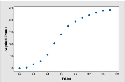
the last row). Data were analyzed using a software for the statistical analyses; the scatterplot has a characteristic distribution, represented in Figure 20:

Figure 20 – Scatterplot of acquired frames varying the value of FrLim

Data was interpolated with a third-order function (S-curve). Regression results are

shown in Table 6.

Table 6 – Regression analysis for # of frames / FrLim curve

It is possible to notice values of P-value equal to zero for first, second and third degree FrLim variable, indicating a non-negligible link between FrLim and number of frames acquired and need to use a third-degree regression function. The value of R-sq(adj)

0,9 0,8 0,7 0,6 0,5 0,4 0,3 0,2 250 200 150 100 50 0 FrLim A c q u ir e d F ra m e s

(42)

(99.56) indicates a reliable regression represented by the function:

𝑁𝑢𝑚𝑏𝑒𝑟𝐴𝑐𝑞𝐹𝑟𝑎𝑚𝑒𝑠 = −486.4 ∗ 𝐹𝑟𝐿𝑖𝑚 + 2360 ∗ 𝐹𝑟𝐿𝑖𝑚2_{− 1718 ∗ 𝐹𝑟𝐿𝑖𝑚}3

In order to validate the regression function, the normality analysis of standardized residuals is done, giving this result in Figure 21:

Figure 21 – Probability plot of standardized residuals

Also, the analysis of standard residuals on the fits, shows that the regression function is reliable, as presented in Figure 22:

Figure 22 – Scatterplot of SRES vs FITS

Dealing with this graph, it is possible to graphically notice the lack of any systematic deviation from the assumption of standardized residuals normality (confirmed by the high value of P-value), validating the regression process.

In order to obtain the minimum optimum threshold value FrLim, the idea is to consider

12 10 8 6 4 2 0 2,5 2,0 1,5 1,0 0,5 0,0 -0,5 -1,0 -1,5 FITS S R E S

(43)

the flex point with oblique tangent. This point, obtained deriving twice the function and placing it equal to 0, coincide with the point in which the change of concavity is present, as well as the point of the curve with the steepest tangent. Steep tangent indicates high increase of acquired frames correlated with small increase of FrLim, so this FrLim value represent the minimum value that has to be considered.

Figure 23 – Tangent steepness reduction after minimum FrLim

For all the acquisitions analyzed, the value of FrLim in correspondence of the flex point is calculated. Considering this single acquisition, the flex point corresponds to FrLim equal to 0.4579. The same operation is done for all the other tests obtaining a mean FrLim value in correspondence of the flex point equal to 0.4496, value that is set as general minimum value of FrLim suggested. This value of FrLim, considering a minimum mean value of ScorePerFrame equal to 0.275 and a maximum one equal to 0.907, represent a displacement from the best acquisition of the 27.5%. As can be seen from the scatterplot, the use of FrLim equal to 0.45 leads to a small number of frames respect to the totality, so if the acquisition frequency is low, in order to have a considerable number of frames examinable, it is advisable to use a higher FrLim, up to a value of 0.55, representing a displacement from the “optimum” skeleton of 44%. Obviously, the quality of the skeletons decreases. Using these values, it is possible to obtain the following skeleton representation in time, cleaned from the non-reliable frames.

(44)

An example of an acquisition after the windowing function is presented in Figure 24:

Figure 24 – Windowed dynamic acquisition

2.1.4 Discussion

As expected, it is possible to notice that, for smaller values of FrLim, the number of considered frames is lower. This is due to the fact that, for smaller indexes value, less dissimilarity from the reference static acquisition are guarantee and a higher number of frames are rejected.

Quality of the skeletons is directly correlated to the number of them: the lower the number of skeletons considered reliable, the higher is the quality.

(45)

2.2 Person Recognition

Person recognition, despite the order in the thesis work constructed on time history development, is exploited in the system before windowing and it is based on some concepts seen previously. Set of the threshold for FrLim is obtained taking one reference person fixed and varying all the dynamic acquisitions (both of the same person and of the other people).

For every dynamic acquisition the parameters discussed in the previous chapter are evaluated and, again, a key point is constituted by the parameter ScorePerFrame. The idea is to find a value of FrLim which can bring the recognition of at least one of the dynamic acquisition corresponding to the correct person, and zero for all the others. For this reason, FrMin, the minimum value of the frame index ScorePerFrame, is considered.

2.2.1 Results

Ten walks for seven people are analyzed with FrLim equal to 0.20, 0.25, 0.30 and 0.35. Number of frames with a score lower than FrLim are gathered for each acquisition and used to understand the global level of successful recognitions. Four conditions can occur:

1) The subject of the dynamic acquisition is the same of the static reference and the system acquires at least one frame: SUCCESS

2) The subject of the dynamic acquisition is the same of the static reference and the system doesn’t acquire any frame: FAIL

3) The subject of the dynamic acquisition is not the same of the static reference and the system doesn’t acquire any frame: SUCCESS

4) The subject of the dynamic acquisition is the same of the static reference and the system acquire at least one frame: FAIL

In the following table (Table 7) the successful rate in percentage for tests combining the same subject for static and dynamic acquisitions, varying FrLim.

(46)

Table 7 – Successful rate in percentage for tests combining the same subject for static and dynamic acquisitions, varying FrLim

In the following Table 8, the successful rate in percentage for tests combining the different subjects for static and dynamic acquisitions, varying FrLim:

Table 8 – Successful rate in percentage for tests combining different subjects for static and dynamic acquisitions, varying FrLim

2.2.2 Discussion

As expected, the threshold value for FrLim is a trade-off between the successful rate for cases in which the subject of the dynamic acquisition is the same of the static reference and the system acquires at least one frame, and the ones in which the subject of the dynamic acquisition is not the same of the static reference and the system doesn’t acquire any frame.

Increasing FrLim from 0.20 to 0.35, the successful rate (same static-dynamic) raises from 34.3% to 95.7% while the other (different static-dynamic) decreases from 98.9% to 79.7%.

A low successful rate for the first case entails that some potentially useful acquisitions are not analyzed, while, for the second case, means that acquisitions of people different from the subject of the static acquisition who enter in the ToF camera’s field of view are analyzed and results are also collected in the history data.

0.2 0.25 0.3 0.35 P01 99 89 80 66 P02 100 100 100 100 P03 93 74 70 55 P04 100 97 88 68 P05 100 99 98 96 P06 100 99 95 86 P07 100 100 97 87 TOT 98,9 94,0 89,7 79,7 Fr

(47)

3 Human Body Parameters of Interest

To analyze walking, sitting and fall detection it is necessary to perform preliminary analyses on the raw skeleton data. These parameters are described in this chapter.

3.1 Parameters

In the following, the main input and output parameters of interest related to different tests are described, separated in walking, sitting and fall detection.

3.1.1 Walking

For the evaluation of walking tests, the joints related to the lower part of the body are considered. In particular:

 Spine base: joint 1

 Hip left and right: joints 13 and 17  Knee left and right: joints 14 and 18  Ankle left and right: joints 15 and 19  Foot left and right: joints 16 and 20

In the first part of the study, these parameters are used to understand if the Kinect V2 camera can be a reliable instrument for gait analysis. After this essential step, they are used to gather gait’s information through different tests made in different conditions. The parameters of interest related to the gait analysis are (Xu et al. 2015):

 Stance time: foot contact time with the ground  Swing time: foot time of flight

 Stride time: time required to obtain a complete step (heel-heel for the same foot)  Step Asymmetry: difference in left and right foot’s swing and stance time;  Step length: calculated as distance heel-to-heel of the foot during the walk;  Foot speed: speed of the foot during the phases of swing;

(48)

 Mean walk velocity: mean velocity of the spine base joint.

 Vertical oscillation amplitude: amplitude of the oscillation of the spine base joint during the walk.

 Vertical oscillation frequency: frequency of the oscillation of the spine base joint during the walk.

 Lateral oscillation amplitude (or Lateral torso lean angle): lateral displacement of the spine base joint during the walk respect to body’s trajectory.

3.1.2 Sitting

For the evaluation of sitting tests, the main joints taken into account are:  Head: joint 4

 Spine Mid: joint 2  Spine Base: joint 1

The study of trajectories and velocities of considered joints are fundamental for the extrapolation of information about the characterization of movements during the sitting. Different tests in different conditions are performed to understand if ToF camera is able to sense common trends which could describe the sitting phase. The parameters of interest are:

 Center of mass overall displacement

 Elevating and sitting down velocity: through analysis of main joints (head, base spine)

 Vertical and lateral displacement

All these parameters are studied looking for analogies between tests.

3.1.3 Fall Detection

Fall detection topic has to be carefully analyzed in order to avoid false alarm related to a wrong data interpretation. Nevertheless, non-revelation of the falling is more serious

(49)

than the false alarm. The fall has been identified with different methods:

 Relative positon of the center of mass’s projection on the ground respect to a circle created using the two feet as extremities of the diameter. Fall is detected when the center of mass projection is outside from the considered circle for every time frame

 Relative distance between body’s center of mass (spine base, joint 1) and the ground. Ground’s coordinates are acquired directly from the ToF camera, so this system works independently from the position and relative distance camera-ground

 Head’s vertical acceleration (joint 4) respect to a threshold value

 Body’s torso angle respect to a threshold value. The torso vector is calculated as difference between spine shoulder (joint 21) and spine base (joint 1)

(50)

3.1.4 Upper Body

The activity is focused on the reconstruction of the posture of the upper body part, as explained in Figure 25:

Figure 25 – Focusing on upper body part

The characteristic angles to be measured to reconstruct movements of the workers are: 1. Right and left shoulder angle

 Beta: Flection (+) / Extension (-)  Alpha: Abduction (+) / Adduction (-) 2. Right and left elbow angle

 Delta: Flection (+) / Extension (-)

 Epsilon: Forearm supination (+)/ forearm pronation (-) 3. Right and left wrist angle

 Tau: Flection (+) / Extension (-)  Nu: Radial (+) / Ulnar (-)

(51)

Angles are illustrated in Figure 26.

Figure 26 – Angles of interest for shoulder, elbow and wrist

0°

Extention

Flection

ζ

0°

Radial

Ulnar

η

0°

Extension

Flection

ε

δ

Supination

Pronation

0°

Wrist Angles

Elbow Angles

0°

Extension

Flection

β

0°

Adduction

α

Shoulder Angles

Abduction

(52)

3.2 Algorithms and Methods

This section describes the algorithms used to evaluate the parameters of interest related to the different situations.

3.2.1 Skeleton Data Manipulation

All tests performed need the evaluation of the coordinates and time history of the skeleton coming from the ToF camera. In order to work with reliable data, some common algorithms are implemented, prerequisite for all the others. After person recognition and windowing, in which the skeleton matrix and the time vector are “cleaned” by frames considered unreliable, data resampling, representation in Kinect reference system, representation in ground reference system and representation in trajectory reference system are performed. A schematic representation of the analysis by steps is available in Figure 27:

Figure 27 – Schematic representation of the analysis by steps

3.2.1.1 Data Resampling

The first passage after the windowing is the data resampling, allowing to work with a consistent number of frames and to consider a fixed acquisition frequency of 30 Hz, that allows creating a time vector evenly spaced. The need of a data resampling derives from the fact that the frame rate of the infra-red TOF camera is limited by the framerate of the standard (visible range) camera.

Skeleton Coordinates Ground Ref. Resampling Skeleton Time History Person Rec. Windowing Traj. Ref. Kinect Ref. Gait Analysis Bar. Analysis Fall Detection

(53)

A schematization of the situation before and after data resampling is available in Figure 28:

Figure 28 – Schematization of the situation before and after data resampling

From a mathematical and informatics point of view, data resampling is implemented through the function Skel3D_Resample that needs in input the skeleton matrix (Skel3D), the time vector (TimeOrigin) and the desired resampling frequency (Freq_Resamp). This function defines a new time vector dividing the considered time interval defined by the vector TimeOrigin in intervals given by 1/ Freq_Resamp. Every joint’s path (in coordinates x, y, z) in function of the old-time vector is known, so through a spline interpolation a relationship between positions in the new time frame can be found. As a result, after data resampling, a new matrix Skel3D and a corresponding time vector

Time are available.

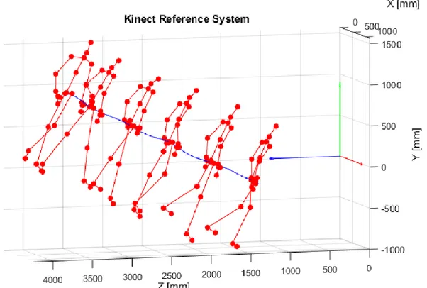
3.2.1.2 Skeleton in Kinect Reference System

From the beginning to the end of the data resampling, Skel3D in function of the time vector, is given in the original Kinect reference system. The skeleton matrix hasn’t undergone any transformation so the reference system is still the camera’s one. As it can be seen in Figure 29, the skeleton representation is not immediately understandable: the lack of ground plane and an inclination of the skeleton’s trajectory due to the height and inclination of the Kinect camera generate an image not suitable for the successive analysis. t [s] Before resampling After resampling t0 tn ∆tf ∆tf ∆t₂ ∆t_m ∆t1 ∆tf ∆tf= 1/30s

Biomechanical analysis using the skeleton measured by the Microsoft Kinect V2

POLITECNICO DI MILANO

School of Industrial and Information Engineering

Master of Science in Mechanical Engineering

Biomechanical Analysis Using The Skeleton Measured By

The

Microsoft Kinect V2

Table of Contents

Table List

Figure List

1. Introduction

1 Human Motion Tracking Systems

1.1 Time of Flight Cameras (ToF)

1.1.1 Basic Principles

1.1.2 Sensors

1.1.3 Microsoft Kinect One (V2) Full Specifications and Software

1.1.4 Considerations

1.2 Home Environment

Commercial

Software

1.3 Work Environment

2 Windowing and Person Recognition

2.1 Windowing

2.1.1 Static Acquisition

2.1.2 Dynamical acquisition

2.1.3 Results

2.1.4 Discussion

2.2 Person Recognition

2.2.1 Results

2.2.2 Discussion

3 Human Body Parameters of Interest

3.1 Parameters

3.1.1 Walking

3.1.2 Sitting

3.1.3 Fall Detection

3.1.4 Upper Body

0°

Extention

Flection

ζ

0°

Radial

Ulnar

η

0°

Extension

Flection

ε

δ

Supination

Pronation

0°

Wrist Angles

Elbow Angles

0°

Extension

Flection

β

0°

Adduction

α

Shoulder Angles

Abduction

3.2 Algorithms and Methods

3.2.1 Skeleton Data Manipulation