Planck stars: theory and phenomenology

(1)

Alma Mater Studiorum ¨ Universit`

a di Bologna

Scuola di Scienze

Corso di Laurea Magistrale in Fisica

Planck Stars

Theory and Phenomenology

Relatore:

Prof. Roberto Casadio

Correlatore:

Dott. Simone Speziale

Presentata da: Andrea Giusti

Sessione II

(2)

(3)

Abstract

General Relativity (GR) is one of the greatest scientific achievements of the 20th century along with quantum theory.

Despite the elegance and the accordance with experimental tests, these two theories appear to be utterly incompatible at fundamental level.

Black holes provide a perfect stage to point out these difficulties. Indeed, classical GR fails to describe Nature at small radii, because nothing prevents quantum mechanics from affecting the high curvature zone, and because classical GR becomes ill-defined at r “ 0 anyway. Rovelli and Haggard have recently proposed a scenario where a negative quantum pressure at the Planck scales stops and reverts the gravitational collapse, leading to an effective “bounce” and explosion, thus resolving the central singularity. This scenario, called Black Hole Fire-works, has been proposed in a semiclassical framework.

The purpose of this thesis is twofold:

• Compute the bouncing time by means of a pure quantum computation based on Loop Quantum Gravity;

• Extend the known theory to a more realistic scenario, in which the rotation is taken into account by means of the Newman-Janis Algorithm.

(4)

(5)

Sommario

La Relativit´a Generale costituisce, assieme alla Meccanica Quantistica, una delle pi´u grandi conquiste del ventesimo secolo.

Tuttavia, nonostante la loro eleganza formale e la loro compatibilit´a con i risultati sperimentali, queste due teorie risultano essere fortemente incompatibili a livello fondamentale.

I buchi neri costituiscono il palcoscenico perfetto per evidenziare le difficolt´a sopracitate. In-fatti, come ben noto, la Relativit´a Generale non risulta essere in grado di descrivere adeguata-mente la Natura per piccoli valori del raggio, e risulta essere mal definita per r “ 0.

Recentemente, Rovelli e Haggard hanno proposto un modello in cui una pressione negativa, di natura puramente quantistica, possa presentarsi una volta raggiunta la cosiddetta densit´a di Planck, interrompendo cos´ı il collasso gravitazionale e causando un “rimbalzo” effettivo ed una conseguente esplosione, risolvendo dunque il problema della singolarit´a centrale che caratter-izza la teoria classica dei buchi neri.

Le finalit´a della presente tesi sono le seguenti:

• Valutare il tempo di rimbalzo, ad oggi noto solo in un contesto semi-classico, per mezzo di un calcolo basato sulla Loop Quantum Gravity;

• Estendere i risultati di Rovelli e Haggard al caso rotante per mezzo dell’algoritmo Newman-Janis.

(6)

(7)

Introduction

It has been a long-standing challenge for theoretical physicists to construct a consistent theory of quantum gravity. It is well known that General Relativity itself gives some hints of its own limits, since given smooth initial data can evolve into singular field configurations.

Classically, this is not a problem at all if the singularities are hidden behind event horizons, because this would mean that these singularity are not in causal contact with the rest of the Universe. This idea, indeed, led Roger Penrose to formulate the so called “weak cosmic censorship conjecture” in 1969.

The 70s have indeed represented a turning point for black hole physics. In this period Stephen Hawking showed, under very general assumptions, that if we take into account the vacuum fluctuations in a region close to the event horizon it follows that black holes emit particles. One of the most remarkable consequences of this result is that the radiation described above is exactly thermal and contains no information about the state of the black hole. This led to the notorious problem of “information loss”, since particles can fall in carrying information but what comes out is featureless thermal radiation.

It can be easily argued that this paradoxical situation would lead to non-unitary evolution of the quantum states, so that one of the basic principles of quantum mechanics would be violated. Another great achievement obtained in the seventies is that black holes can be treated, at least formally, as thermodynamic-like systems. Indeed, they have an entropy and a temperature which are given by

TH “ ~ κ 2π kB , SBH“ kBA 4`2 P

where κ is the surface gravity and A is the area of the horizon.

These quantities appear to be closely related to the quantum aspects of gravitation, in the sense that they depend on both Planck’s constant ~ and Newton’s constant G. The Hawking temperature, as well as the Bekenstein-Hawking entropy, have been derived in many indepen-dent ways, in different settings and with different assumptions, so that they are considered robust features to be included in any complete theory of quantum gravity.

Although none of these results deal directly with the problem of the curvature singularity, which represents the emblematic example of a region characterized by pure quantum features, these quantities can still be extremely useful to determinate whether a theory of quantum gravity is, more or less, worth of trust.

Nowadays, there are different approaches to quantum gravity in which it has been possible to recover the former quantities by means of a pure quantum computation, such as Loop Quantum Gravity, String Theory, Asymptotic Safety and others.

(12)

x CONTENTS However, despite the degree of progress of these theories, quantum gravity still remains a major unsolved challenge at the core of fundamental physics and its phenomenology is still beyond direct observations. However, recent research has brought to surface a number of different ideas for indirect tests, and the possibility of detecting effects that occur in the Planck scale regime does not appear completely out of reach. For example, the idea that quantum mechanical effects may resolve the gravitational singularity has led to the notion of Planck stars, and its associated phenomenology currently under exploration, as well as the possibility that black holes are quantum condensates resolves most of the issues encountered in the literature.

The aim of this thesis is to give a first look at which kind of predictions can be recovered by a recently proposed model for non-singular black holes. Moreover, we are also interested in the consequences deriving from the application of loop quantum gravity to the quantum core of such compact self-gravitating object.

In order to be more specific, in Part I: Prologue we present the classical description of black holes. In this context we also introduce the most peculiar paradoxes known in the (semi)classical theory of black holes, with particular regards for the paradox of information loss and for the emergence of singularities in general relativity. As discussed above, these issues lie at the very foundation of black hole physics, and represent one of the main motivation for the development of the different approaches to quantum gravity. Moreover, in the Prologue we introduce two different and complementary semiclassical scenarios derived by analogy with loop quantum cosmology, i.e. the Planck Star model and Black Hole Fireworks, aimed to resolve the the previously mentioned oddities of the “classical” theory.

In Part II: On the Effective Metric of a Rotating Planck Star, we present a generalization of the known results for the Planck Star model. In particular, our aim is to recover an effective description of the spacetime surrounding a rotating Planck Star in order to provide a more realistic physical description such a star-like object. To do so we use the renowned Newman-Janis Algorithm.

Finally, in Part III: Black Hole Fireworks and Transition Amplitudes in Loop Quantum Gravity, firstly we introduce some basic aspects of the Spinfoam Approach to quantum gravity. Secondly, we analyse in details the Lorentzian EPRL model also providing some generalized rules for computing transition amplitudes in loop quantum gravity. Then, we present a poten-tial application to these techniques to the problem of the computation of the bouncing time for black hole fireworks together with a more realistic description of the boundary spin-network for this scenario. However, the implementation of these computations is left for a future study.

(13)

CONTENTS xi AcknowledgementsI would like to take this opportunity to thank the various individuals to whom I am indebted, not only for their help in preparing this thesis, but also for their support and guidance throughout my studies. The particular choice of topic for this thesis proved to be very rewarding as it allowed me to explore many interrelated areas of Physics and Math-ematics that are of great interest to me. Thus I would first like to extend my thanks to my supervisors, Prof. Roberto Casadio and Dr. Simone Speziale, for encouraging me to pursue this topic and for providing me with very friendly and insightful guidance when it was needed. I am also extremely grateful to Prof. Carlo Rovelli for welcoming me into his research group in Marseille. Furthermore, I would also like to thank Hal Haggard, Francesca Vidotto, Alejandro Perez and Tommaso De Lorenzo for very useful discussions.

Finally, I would like to show my gratitude to those who have not directly been part of my academic life yet, but they have been of central importance in the rest of my life. First, and foremost, my parents, Antonella and Maurizio, for their unrelenting support and for teaching me the value of things. Also, to my sisters, Giulia and Giorgia, who have had to deal with my unending rants and other oddities. I would also thank some of my dearest friends, in particular Simone, Margherita and Martina, for their help and support during some very tough moments of the last couple of years as well as during the preparation of this thesis. I also offer my thanks and apologies to my girlfriend, Claudia, for putting up with months of me working on my thesis and with my endless, uninteresting updates on the latest traumatic turn of events. You are as kind as you are beautiful.

This work is dedicated to the loving memory of the greatest man I have ever known, my grandfather Marcellino, and to my grandmother Margherita.

(14)

xii CONTENTS

I have nothing to offer but blood, toil, tears, and sweat. Winston Churchill

I don’t pay attention to the world ending.

It has ended for me many times and began again in the morning. Nayyirah Waheed

Once the game is over the king and the pawn go back into the same box.

Per quanto mi riguarda, mi sembra di essere un ragazzo che gioca sulla spiaggia e trova di tanto in tanto

una pietra o una conchiglia pi´u belle del solito,

mentre il grande oceano della verit´a resta sconosciuto davanti a me. Sir Isaac Newton

(15)

Part I

Prologue

(16)

(17)

Chapter 1

Introduction to Black Holes

The aim of the first part of this thesis is to review some classical and semi-classical results known in Black Hole physics which are going to be discuss and analysed extensively later. Most of this introductory part is based on [1; 2; 3]. We have also drawn on some ideas from the books [4;5].

In this work we choose to use the metric signature p` ´ ´ ´q. Moreover, throughout most of this thesis we shall use the so called geometrized units, i.e. c “ ~ “ G “ 1. However, we are going to restore the values of G, ~ and c whenever necessary in order to make explicit estimates.

1.1 Spherical Symmetry

It is quite known that the only way to address the Cauchy Problem for the Einstein’s Field Equations is to assume some underlying symmetries of the spacetime.

The most obvious assumption is then to consider a spherically symmetric gravitational field. Indeed, this assumption represents a quite good approximation for the gravitational field cre-ated by a star, at least in the far field limit.

Let us now give a proper mathematical characterization of the concept of Spherical Sym-metry.

From the fundamental courses of Linear Algebra and Geometry it is well known that the set of all isometries of a metric space forms a group. Consider the line element on the 2-sphere, S2_:

dΩ2 “ dθ2` sin2θ dφ2 (1.1) The set of all the transformations that leaves this line element unchanged, i.e. the isometry group for the 2-sphere given the former metric, is called Orthogonal Group, Op3q. For sake of generality, if we consider the matrix representation of this group, we have that

Opnq “ A P GLpnq : AAT

“ I(

It is straightforward to conclude that Opnq has has two connected components.

Indeed, let A P Opnq. Since detA “ detAT _{we have, due to the Binet’s theorem, that}

detA “ ˘1. So that we have one connected component that contains orthogonal matrices 3

(18)

4 CHAPTER 1. INTRODUCTION TO BLACK HOLES whose determinant is one, known as the Special Orthogonal Group, SOpnq, and the other that contains orthogonal matrices whose determinant is minus one. Moreover, SOpnq is the only subgroup of Opnq connected with the identity operator.

Thus, both SOpnq and Opnq are Lie Group.

For our purpose, we are interested in the set of isometries that does not include reflections of the axes, indeed we are only concerned about the invariance under rotations, at least for what concerns the spherical symmetry.

Given the former discussion, we can then define a spherically symmetric spacetime as follows. Definition 1. A spacetime is said to be spherically symmetric if its isometry group contains an SOp3q subgroup whose orbits1 _{are 2-spheres.}

In such spacetime we can define the radial coordinate in an unambiguous way. Indeed, let M be a spherically symmetric spacetime, thus we are allowed to define the so called area-radius function r :_{M ÝÑ R such that rppq “}aAppq{4π , @p P M, where Appq is the area of the S2

orbit through p P M .

1.2 Static and Stationary Spacetimes

Definition 2. A spacetime p_{M, gq is said to be stationary if it admits a Killing vector field} k which is everywhere timelike, i.e. gpk, kq ą 0

Now, if we consider a hypersurface Σ Ă_{M nowhere tangent to k, we are allowed to choose} the coordinate as follows:

• Let xi_{, i “ 1, 2, 3 be coordinates on Σ;}

• Now assign coordinates pt, xi

q to the point parameter distance t along the integral curve of k that starts at the point with coordinates xi _{on Σ}

This defines a coordinate chart pt, xi_{q ” pt, xq at least in a neighbourhood of Σ.}

In such a coordinate chart we have that k “ B{Bt. Since k is a Killing vector field, we can cast the metric of the spacetime in such a way that it shall appear as independent from the coordinate t, hence

ds2“ g00pxq dt2` 2g0ipxq dtdxi` gijpxq dxidxj (1.2)

with g00pxq ą 0.

Next we need to introduce the notion of hypersurface-orthogonality. Let Σ be a hypersurface specified by f pxq “ 0, where f : M ÝÑ R is a smooth function such that df ‰ 0 on Σ. Then, df is normal to Σ. Indeed, if T is a vector tangent to Σ, thus df pT q “ T f “ Tα

Bαf “ 0

because f is constant on Σ.

Any other 1-form n normal to Σ can be written as n “ gdf ` f n1 _{where g is a smooth function}

1

The orbit of a point under a group of diffeomorphisms is the set of points that can be reached by the starting point by acting on it with all of the diffeomorphisms.

(19)

1.3. THE SCHWARZSCHILD BLACK HOLE 5 with g ‰ 0 on Σ and n1 _{is a smooth 1-form.}

So, if n is normal to Σ then:

n ^ dn|_Σ“ 0 Conversely,

Theorem 1 (Frobenius). If n ‰ 0 is a 1-form such that n ^ dn “ 0 everywhere then

Df, g : M Ñ R such that n “ g df so n is normal to surfaces of constant f i.e. n is hypersurface-orthogonal.

Given this fundamental concept, we can now define a static spacetime as follows:

Definition 3. A spacetime is static if it admits a hypersurface-orthogonal timelike Killing vector field.

Remark. It is straightforward to notice that a static spacetime is also stationary.

For such a spacetime, we know that k is hypersurface-orthogonal so when defining adapted coordinates we can choose Σ to be orthogonal to k. At the same time, Σ is the surface at t “ 0, with normal dt. Thus we must have that kα “ gαβkβ9p1, 0q which implies that ki “ 0. Hence,

ki“ giαkα “ gi0k0 “ gi0pxq “ 0 from which we conclude that gi0pxq “ 0.

Therefore, in adapted coordinates a static metric takes the form

ds2 “ g00pxq dt2` gijpxq dxidxj (1.3)

with g00pxq ą 0.

It is quite obvious to notice that static then means time-independent and invariant under time reversal. Both of these properties result to be fundamental in the formulation of the model of Black Hole Fireworks.

1.3 The Schwarzschild Black Hole

We are interested in determining the gravitational field of a time-independent spherical ob-ject so we assume our spacetime to be stationary and spherically symmetric. It can be shown (as a part of the Birkhoff’s theorem, see below) that any such spacetime must actually be static. The Schwarzschild metric (1916) is a solution to the vacuum Einstein’s Field Equations, i.e. Rµν “ 0, and it is given by

ds2“ ˆ 1 ´2m r ˙ dt2´ ˆ 1 ´2m r ˙´1 dr2´ r2dΩ2 (1.4) where 0 ă r ă 8 is defined as above and dΩ2

“ dθ2` sin2θ dφ2 is the round metric on S2. The line element (1.4) is the unique spherically symmetric solution to the vacuum Einstein’s equations. This result is known as Birkhoff’s theorem and it has strong implications.

More precisely,

Theorem 2 (Birkhoff). Any spherically symmetric solution of the vacuum Einstein equation is isometric to the Schwarzschild solution.

(20)

6 CHAPTER 1. INTRODUCTION TO BLACK HOLES Remark. It is important to notice that k “ B{Bt is timelike for r ą 2m so, in this region, the Schwarzschild solution is static.

Birkhoff’s theorem implies that the spacetime outside any spherical body is described by the time-independent exterior Schwarzschild solution. This is true even if the body itself is time-dependent. Moreover, the spacetime outside the star will be described by the static Schwarzschild solution even during the collapse.

Let us then study the features of the most important type of geodesics, i.e. the radial null geodesics. These curves are defined by the following properties:

ds2 “ 0 , dθ “ dφ “ 0 So, the line element (1.4) reduces to

0 “ ˆ 1 ´2m r ˙ dt2´ ˆ 1 ´2m r ˙´1 dr2 Then, if we introduce the Regge-Wheeler radial coordinate r˚_{, defined as}

dr˚

“ dr

2

1 ´2m r

Along a radial null geodesic we have

dt dr˚ “ ˘1

and then

t ¯ r˚

“ const. Remark. The coordinate r˚

“ r˚prq is often called tortoise coordinate, because r˚ changes only logarithmically close to the horizon. This coordinate change maps the range r P p2m, 8q of the radial coordinate onto r˚ _{P R.}

We can now define a new coordinate

v “ t ` r˚

which is manifestly constant along ingoing radial null geodesics.

If we then want to use pv, r, θ, φq as coordinates, we could eliminate t from the line element (1.4) by the substitution t “ v ´ r˚_{. Hence, the Schwarzschild metric shall be recast as follows:}

ds2 “ ˆ 1 ´2m r ˙ dv2 ´ 2dvdr ´ r2dΩ2 (1.5) The latter is then the Schwarzschild metric written in terms of the so called ingoing Eddington-Finkelstein (EF) coordinates.

Unlike the metric components in Schwarzschild coordinates, the components of the above ma-trix are smooth for all r ą 0, in particular they are smooth at r “ 2m.

The Schwarzschild spacetime can now be extended through the surface r “ 2m to a new region with r ă 2m. Moreover, it is obvious to see that the new line element is still a solution

(21)

1.3. THE SCHWARZSCHILD BLACK HOLE 7 of the vacuum Einstein’s equation also in this new region.

If we now call λ the affine parameter for these radial null geodesics, then one can easily deuce the geodesic equations for the Schwarzschild spacetime, i.e.

dt dλ “ ˆ 1 ´2m r ˙´1 , dr dλ “ ˘1

where the upper sign corresponds to outgoing geodesics, i.e. increasing r, and the lower is for the ingoing one.

The ingoing radial null geodesics in the EF coordinates are then defined by v “ const. , dr

dλ “ ´1

Hence such geodesics will reach r “ 0 in finite affine parameter. Since the metric is Ricci flat, the simplest non-trivial scalar constructed from the metric is the Kretschmann scalar, i.e.

K “ Rµνρσ_R µνρσ “

48m2

r6 (1.6)

That diverges as the radius approaches zero. Since this is a scalar, it diverges in all charts. Therefore there exists no chart for which the metric can be smoothly extended through r “ 0. This is a clear example of a curvature singularity, where tidal forces become infinite and the known laws of physics break down.

Remark. Recall that for r ą 2m, the Schwarzschild solution admits the Killing vector field k “ B{Bt. If we now change the coordinates to the ingoing EF coordinates we get that

v “ t ´ r˚ ùñ k “ B Bt “ Bv Bt B Bv “ B Bv

We can then use this definition in order to extend k to r ď 2m. It is easy to see that k2

“ gµνkµkν “ gvv, which means that k is null at r “ 2m and spacelike for r ă 2m. Thus, the

extended Schwarzschild solution is static only for r ą 2m.

So far we have considered ingoing radial null geodesics (v “ const.) in the ingoing EF coordinates. It is then interesting to study the behaviour of the outgoing radial null geodesics in the chart. The latter, for r ą 2m, are given by u “ t ´ r˚

“ const..

The simpler way to understand the underling physics behind this problem is to plot the radial null geodesics on a spacetime diagram. In particular, if we define t˚

“ v ´r, consequently the ingoing radial null geodesics are straight lines at 45˝ _{in the pt}˚_{, rq plane.}

(22)

8 CHAPTER 1. INTRODUCTION TO BLACK HOLES This gives the so called Finkelstein diagram for the Schwarzschild metric in the ingoing EF coordinates.

It is clear from the plot that the outgoing radial null geodesics have increasing r if r ą 2m. But if r ă 2m then r decreases for both families of null geodesics. Both reach the curvature singularity at r “ 0 in finite affine parameter. Since nothing can travel faster than light, the same is true for radial timelike curves. Consequently, there is no signal that can be sent from a point with r ă 2m to a point with r ą 2m. This is, indeed, the defying feature of a Black Hole. More precisely, a Black Hole is a region of an asymptotically flat spacetime from which we are not able to send a signal to infinity.

1.4 The Black Hole region

At this stage, we could try to characterize the black hole region in a more precise mathematical way. But first, we need to recall some important definitions.

Definition 4. A vector V is causal if it is timelike or null, i.e. V2

ě 0. A curve is causal if its tangent vector is everywhere causal.

Let p_{M, gq be a spacetime. At each point p P M, the tangent space T}pM is clearly

isomor-phic to the Minkowski spacetime. Thus, at any point of a spacetime, the metric determines two light-cones in the tangent space at that point2_{. Our aim is to regard one of these as the}

future light-cone and the other as the past light-cone. To do so we can, for example, pick a causal vector field and define the future light-cone to be the one in which it lies, thus

Definition 5. A spacetime is time-orientable if it admits a time-orientation, i.e. a causal vector field T . Then, a causal vector V is future-directed if it lies in the same light cone as T and past-directed otherwise.

Remark. Any other time orientation is either everywhere in the same light-cone as T or ev-erywhere in the opposite light-cone. Hence a time-orientable spacetime admits exactly two inequivalent time-orientations.

For example, for the Schwarzschild metric in the ingoing EF coordinates ξ “ B{Br is globally null, indeed ξ2

“ grr “ 0 , @p P M, hence defines a time-orientation. Therefore we can use ξ

to define our time orientation for r ą 0.This is not the case for k “ B{Bt “ B{Bv because it is

2_{It is very important to empathize that the light-cone of p is a subset of T}

(23)

1.5. EXTENDIBILITY& THE KRUSKAL SPACETIME 9 timelike for r ą 2m, null for r “ 2m and spacelike for r ă 2m.

All this discussion results to be important in the proof of the following fundamental property of the Schwarzschild metric in the ingoing EF coordinates:

Proposition 1. Let xµ_{pλq be any future-directed causal curve. If Dλ}

0 such that rpλ0q ď 2m,

then rpλq ď 2m , @λ ě λ0.

This result implies that no future-directed causal curve connects a point with r ď 2m to a point with r ą 2m. This statement makes more precise our definition of a black hole. Moreover, the boundary of the black hole region is called the Event Horizon. In particular, it is now straightforward to see that the surface r “ 2m is the event horizon for the Schwarzschild black hole.

1.4.1 White Holes

If we, instead, extend the Schwarzschild spacetime with outgoing Eddington- Finkelstein coor-dinates, i.e. u “ t ´ r˚_{, the line element (}_1.4_{) becomes}

ds2 “ ˆ 1 ´2m r ˙ du2` 2dudr ´ r2dΩ2 (1.7) The same analysis reveals that ingoing photons emitted at r ą 2m or r ă 2m never cross r “ 2m: they approach r “ 2m and hover the horizon forever. Conversely, all outgoing null geodesics escape to infinity. Looking at the light-cones, we see that everything inside r “ 2m is ejected. The region r ă 2m is then called White Hole and r “ 2m is said to be the white hole horizon. It is also important to notice that this is the exact time reversal of a black hole.

1.5 Extendibility

& the Kruskal spacetime

In the previous sections we have shown that the Schwarzschild solution of the vacuum Einstein’s equations can be analytically extended in two different ways, revealing the existence of a black hole region and a white hole region.

It is quite important then to properly empathize the concept of analytic extension in general relativity.

Definition 6. A spacetime pM, gq is said to be extendible if it is isometric to a proper subset of another spacetime p_M1_{, g}1

q. The latter is called an extension of pM, gq. Otherwise, a specetime is said to be not extendible.

A canonical example is given by the relation between the Schwarzschild solution and the Kruskal spacetime.

Let us consider r ą 2m. In this region we can define the Kruskal-Szekeres coordinates pU, V, θ, φq by

U “ ´ exp p´u{4mq , V “ exp pv{4mq (1.8) thus U ă 0 and V ą 0. Note that U V “ ´ exp pr˚ {2mq “ ´ r 2m´ 1 ¯ exp pr{2mq , U V “ ´ exp pt{2mq

(24)

10 CHAPTER 1. INTRODUCTION TO BLACK HOLES which give us an unambiguous determination of r “ rpU, V q and t “ tpU, V q.

Now, it is easy to see that the Schwarzschild spacetime can be rewritten as ds2

“ 32m

3_{exp p´r{2mq}

r dU dV ´ r

2_dΩ2 _(1.9)

One can see by inspection that this new metric can be analytically extended, with non-vanishing determinant, through the surfaces U “ 0 and V “ 0 to the new regions U ą 0 and V ă 0. Moreover, from the defining equations for r and t we can see that the surface r “ 2m is actually two surfaces (U “ 0 and V “ 0) that intersect at U “ V “ 0.

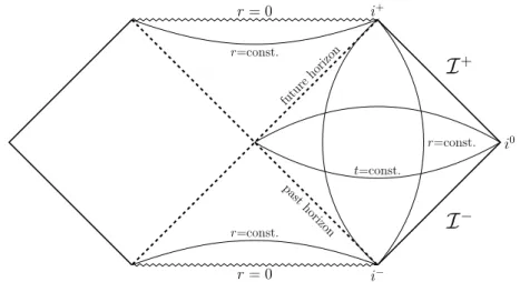
Similarly, the curvature singularity at r “ 0 corresponds to the two branches of the hyperbola given by U V “ 1. This information, together with the causal structure of such a spacetime, can be summarized by the Carter-Penrose diagram of the Kruskal-Szekeres spacetime.

i+ i− i0

I

−

I

+ r = 0 r = 0 future horizon past horizon t=const. r=const. r=const. r=const.

Figure 1.1: Penrose-Carter diagram of the Kruskal-Szekeres spacetime.

The Kruskal-Szekeres spacetime allows us to relate the black hole and the white hole ex-tensions of the Schwarzschild solution. In particular, this spacetime represents the maximal extensionof the Schwarzschild spacetime.

1.6 Some remarks about Singularities

By definition, a metric tensor is said to be singular if, in some basis, its components are not smooth or its determinant vanishes. A coordinate singularity can be eliminated by a change of coordinates, as it happens for the singularity at r “ 2m for the Schwarzschild spacetime. These are unphysical. However, if it is not possible to eliminate the bad behaviour by a change of coordinates then we have a physical singularity. In this chapter we have encountered such singularities while constructing the Kretschmann scalar for the Schwarzschild solution. However, it is also possible to have more general curvature singularities for which no

(25)

1.6. SOME REMARKS ABOUT SINGULARITIES 11 scalar constructed from the Riemann tensor diverges but, nevertheless, there exists no chart in which the Riemann tensor remains finite. Moreover, not all physical singularities are curvature singularities (e.g. conical singularities).

A problem in defining singularities is that they are not “places” of the spacetime with some particular features, they, indeed, do not belong to the spacetime manifold at all, due to the fact that we define spacetime as a pair pM, gq where g is a smooth Lorentzian metric.

A common property of singularities is that there must exist some geodesics that cannot be extended to arbitrarily large affine parameter because they “end” at the singularity. It is this property that we will use to define what we mean by “singular”.

Definition 7. p P_{M is a future endpoint of a future-directed causal curve γ : pa, bq Ñ M} if, for any neighbourhood O of p, there exists t0P R such that γptq P O , @t ą t0. We say that

γ is future-inextendible if it has no future endpoint. Similary for past endpoints and past inextendibility. γ is inextendible if it is both future and past inextendible.

Definition 8. A geodesic is complete if an affine parameter for the geodesic extends to ˘8. A spacetime is geodesically complete if all inextendible causal geodesics are complete.

One can easily convince himself that a spacetime that is extendible will also be geodesically incomplete. However, the Kruskal spacetime is both inextendible, being the maximal extension of the Schwarzschild spacetime, but nonetheless geodesically incomplete because one can always find a geodesic that hits r “ 0 in finite affine parameter. So we will regard a spacetime as singular if it is geodesically incomplete and inextendible.

(26)

(27)

Chapter 2

Causal Structure and Predictability

Almost every physical problem can be cast as an initial value problem. In particular, if we are interested in knowing the state of a system at some moment in time, provided the state of the system at an earlier time and the laws of physics (encoded in a set of partial differential equations), the fact that such a problem makes sense is due to the concept of causality, i.e. the idea that future events can be understood as consequences of certain initial conditions coupled with the laws of physics.

In this chapter we will quickly review some of the most relevant concepts used in understanding how causality works in general relativity and how it relates with black hole physics. In this chapter we shall look at the problem of evolving matter field on a fixed background spacetime, rather the the evolution of the metric itself. Our guiding principle will be that no physical signals can travel faster then light, therefore information will only travel along null or timelike trajectories.

Definition 9. Let p_{M, gq be a time-orientable spacetime and S Ă M. The chronological} futureof S, denoted I`_{pSq, is the set of points of}_{M which can be reached by a future-directed}

timelike curve starting on S. The causal future of S, denoted J`_{pSq, is the union of S with}

the set of points of _{M which can be reached by a future-directed causal curve starting on S.} The chronological past I´

pSq and causal past J´pSq are defined similarly.

Definition 10. Let S Ă_{M. Then S is said to be achronal if no two points in S are connected} by a timelike curve.

Now, if we consider a closed achronal set S Ă M, we can define the future domain of dependence of S, D`

pSq, as the set of all points p PM such that every past moving inex-tendible1 _{causal curve through p must intersect S. It is trivial to notice that, S Ă D}`_{pSq. The}

past domain of dependence, D´_{pSq, is defined in a similar way. Moreover, we can also define,}

roughly speaking, the future Cauchy horizon, denoted H`

pSq, as the boundary of D`pSq; analogously one can also define the past Cauchy horizon, H´_{pSq. It is easy to see that H}˘_pSq

have to be null surfaces.

The usefulness of these definition is due to the fact that, if nothing can travel faster than light, then signals cannot propagate outside the light-cone of any p PM. Hence, if every curve that remains inside this light-cone must intersect S, then the informations specified on S should

1_{It basically means that the cure does not end at some finite point.}

(28)

14 CHAPTER 2. CAUSAL STRUCTURE AND PREDICTABILITY be sufficient to predict the situation at p.

The set of all points for which we can predict what happens by knowing the conditions on S is then given by DpSq “ D`_pSq_{Ť D}´_{pSq, which is simply called Domain of Dependence of}

S.

Definition 11. A closed achronal surface Σ is said to be a Cauchy surface if DpΣq “M. Then, given the initial data on a Cauchy surface we can predict what happens throughout all of spacetime. Nevertheless, in general DpΣq ‰_{M thus solutions of hyperbolic equations will} not be uniquely determined in_{MzDpΣq by data on Σ. Hence, given only this data, there will} be infinitely many different solutions onM which agree within DpΣq. Moreover, one can also define the concept of partial Cauchy surface, which is basically a closed, achronal and edgeless hypersurface of_M.

Definition 12. A spacetime p_{M, gq is globally hyperbolic if it admits a Cauchy surface.} Theorem 3. Let p_{M, gq be globally hyperbolic. Then}

(i) there exists a global time function;

(ii) surfaces of constant t are Cauchy surfaces, and these all have the same topology T ; (iii) the topology of M is R ˆT .

The concept of global hyperbolicity was firstly introduced by Leray in order to consider well-posedness of the Cauchy problem for the wave equation on the manifold. In view of the initial value formulation for Einstein’s equations, global hyperbolicity is seen to be a very natural condition in the context of general relativity, in the sense that given arbitrary initial data, there is a unique maximal globally hyperbolic solution of Einstein’s equations.

2.1 Asymptotically Flat Spacetimes

So far we have seen that it is reasonable to define a black hole, roughly speaking, as the region of spacetime from which no information-carrying signals are allowed to escape to a distant observer. However, in order to make this definition rigorous, one must clarify what class of observers is meant and what is the geometrically invariant meaning of the term “distant”. The necessary refinement is easily achieved in the physically important case in which there is no matter and no sources of fields far from the black hole. The greater the distance from the black hole, the smaller the deviations of the spacetime geometry are from flatness. A spacetime with this property is said to be asymptotically flat.

2.1.1 Conformal Compactification

Consider a spacetime p_{M, gq.}

Definition 13. A conformal transformation is a map such that pM, gq ÝÑ pM, ¯gq gpxq ÞÑ ¯gpxq “ Ω2pxq gpxq where Ω is a smooth positive function on_M.

(29)

2.1. ASYMPTOTICALLY FLAT SPACETIMES 15 The metrics g and ¯g agree on the definitions of timelike, spacelike and null so we have that conformal transformations preserve the causal structure of the spacetime.

The idea of conformal compactification is to choose Ω so that points at infinity with respect to g are at finite distance with respect to the new unphysical metric ¯g. To do this we need Ω Ñ 0 at “infinity”. More precisely, we try to choose Ω so that the spacetime p_{M, ¯gq is part} of a larger unphysical spacetime pM, ¯gq. M is then a proper subset of M with Ω|BM“ 0 in

M. This boundary corresponds to infinity of the physical spacetime.

2.1.2 Asymptotic Flatness

Assuming that the properties of asymptotic flat spaces in the neighborhood of infinity must be similar to those of Minkowski space, Penrose suggested the following definitions.

Firstly, let us define asymptotically simple spacetimes:

Definition 14. A spacetime p_{M, gq is said to be asymptotically simple if there exists} another unphysical space p_{M, ¯gq with boundary BM ” I and a regular metric ¯g such that:}

i M z_{I is conformal to M, and ¯g “ Ω}2_{g in} _M;

ii Ω|_Mą 0, Ω|I “ 0 and BµΩ|_I ‰ 0;

iii Each null geodesic in M begins and ends on I.

The unphysical space M , defined as above, is then called conformal Penrose space.

Let p_{M, gq be an asymptotically simple spacetime, let g be such that Ric “ 0 in the} neigh-borhood ofI and assume that the natural conditions of causality and spacetime orientability are satisfied. Then, pM, gq has the following properties:

1. The topology ofM is R4_;

2. _{I is null and consists of two disconnected components, i.e. I “ I}`_{Ť I}´_{, each}

diffeo-morphic to R ˆ S2_;

3. The generators of the surfacesI˘ _{are the null geodesics in} _M;

The first two results tell us that the global structure of the asymptotically flat space is the same as that of Minkowski space, as we were expecting.

According to [6], in order to take into account the existence of localized regions of strong gravitational fields which do not alter the asymptotic properties of spacetime, it is sufficient to analyse the class of spaces that can be converted into asymptotically simple spaces by removing certain inner regions containing singularities of some kind and by subsequent smooth patching of the resultant holes. Such spaces are said to be weakly asymptotically simple.

Now, a weakly asymptotically simple spacetime is asymptotically flat if its metric in the neighborhood ofI satisfies Einstein’s vacuum equations.

(30)

(31)

Chapter 3

Black Holes

& The Singularity

Theorem

3.1 Formal definition of Black Hole

Now that we have given a proper definition of “infinity” as well as a detailed characterization of the causal structure of a Lorentzian manifold, we can then make more precise our definition of a black hole as a region of an asymptotically flat spacetime from which it is impossible to send a signal to infinity.

Definition 15 (Black Hole). Let pM, gq be a spacetime that is asymptotically flat at null infinity. The black hole region is

B “ M z rM X J´

pI`qs where J´

pI`q is defined by means of the unphysical spacetime pM, ¯gq. The future event horizon is then defined as_H`

“ BB.

The definition which has been just presented can be enlightened by means of a Carter-Penrose diagram. i− i0 i+ singularity H+ I+ I− J−₍_I+₎

Figure 3.1: General Carter-Penrose diagram for an Eternal Black Hole. The black hole region is red-shaded while the future horizon is represented by a dashed line.

(32)

18 CHAPTER 3. BLACK HOLES& THE SINGULARITY THEOREM Similarly, the white hole region is _{W “ M z rM X J}`

pI´qs and the past event horizon is H´

“ BW.

From [1], provided a time-orientable spacetime p_{M, gq, we have the following fundamental} theorems:

Theorem 4. Let S Ă_{M. Then BJ}`

pSq is an achronal 3d submanifold ofM. Theorem 5. Let S Ă _{M be closed. Then every p P BJ}`

pSq with pnotinS lies on a null geodesic γ lying entirely in BJ`_{pSq and such that γ is either past-inextendible or has a past}

endpoint on S.

These theorems tell us that_H˘ _{have to be null hypersurfaces. Moreover, the time reversal}

of the second theorem implies that the generators of_H` _{cannot have future endpoints.}

How-ever, they can have past endpoints (e.g. the point in which a black hole forms in a gravitational collapse of a star). So null generators can enterH` _{but they cannot leave it.}

There is also another technical condition that will be relevant in the following.

Definition 16. An asymptotically flat spacetime pM, gq is said to be strongly asymptoti-cally predictableif there exists an open region V ĂM such that tM X J´_pI`

qu´Ă V , i.e. the closure of_{M X J}´

pI`q is contained in V , and pV , ¯gq is globally hyperbolic.

This definition implies that p_{M X V , gq is a globally hyperbolic subset of M . Roughly} speaking, there is a globally hyperbolic region M X V of spacetime consisting of the region not inB together with a neighbourhood of H`_{. It ensures that physics is predictable on, and}

outside, _H`_{. A simple consequence of this definition is the result that a black hole cannot}

bifurcate, i.e. split into two.

3.2 The Singularity Theorem

The Schwarzschild solution of the Einstein’s field equations clearly tells us that the final stage of a spherically symmetric gravitational collapse might result in the formation of a curvature singularity. It is then interesting to investigate whether such outcome is a feature of the spherical symmetry rather then a property of more general collapses. However, in 1965 Penrose formulated his notorious singularity theorem which basically states that singularities are a generic prediction of general relativity.

3.2.1 Null Hypersurfaces

Null hypersurfaces have an interesting geometry, and play an important role in general relativ-ity. In particular, as we have seen, they represent horizons of various sorts, such as the event horizons. Let pM, gq be be a spacetime.

Definition 17. A null hypersurface is a hypersurface whose normal is everywhere null. Let n be normal to a null hypersurface Σ Ă M. Then any vector X ‰ 0 tangent to the hypersurface obeys n ¨ X ” gµνnµXν which implies that either X is spacelike or X is parallel to

n, i.e. null. In particular, note that n is also tangent to the hypersurface. Hence, the integral curves of n lie within Σ.

(33)

3.2. THE SINGULARITY THEOREM 19 Proposition 2. The integral curves of a are null geodesics. These are called the generators of Σ.

Recalling that a geodesic congruence in U ĂM is a family of geodesics such that exactly one geodesic passes through each p P U , then we can define the null expansion scalar θ of Σ with respect to n as a smooth function on Σ that gives a measure of the average expansion of the null generators of Σ towards the future, and it is defined as the divergence of the vector field n along Σ, i.e. θ “_∇αnα.

While θ depends on the choice of n, it does so in a simple way. Moreover, a positive rescaling of n rescales θ in the same way, i.e. ˜n “ f n ñ ˜θ “ f θ. Thus the sign of the null expansion θ does not depend on the scaling of n; therefore θ ą 0 implies expansion on average of the null generators, and θ ă 0 means contraction on average.

It is useful to understand how the null expansion varies as one moves along a null generator of Σ. Let λ Ñ γ “ γpλq be a null geodesic generator of Σ and assume n is scaled so that γ is affinely parameterized. Then it can be shown that the null expansion scalar θ “ θpλq along γ satisfies the propagation equation,

dθ dλ “ ´Ricpγ 1_{, γ}1 q ´ σ2´1 2θ 2 _(3.1) where γ1

” pdxµ{dλqBµ “ TµBµ, Ricpγ1, γ1q “ RµνTµTν and σ, the shear tensor, measures

the deviation from perfect isotropic expansion. Equation (3.1) is known as the Raychaud-huri’s equationfor a null geodesic congruence and, together with a timelike version, plays an important role in the proofs of the classical Hawking-Penrose singularity theorems.

Equation (3.1) shows how the curvature of space-time influences the expansion of the null generators. Here, we can see, for example, a trivial consequence of this equation.

Proposition 3. Let p_{M, gq be a spacetime which obeys the null energy condition}1 _{and let Σ be}

a smooth null hypersurface in M. If the null generators of Σ are future geodesically complete then the null generators of σ have nonnegative expansion, θ ě 0.

Proof. Suppose θ ă 0 at p P Σ. Let γ : r0, 8q Ñ Σ such that λ ÞÑ γpλq be the null geodesic generator of Σ passing through p “ γp0q. Let also assume γ to be affinely parametrized. Let θ “ θpλq be the null expansion of Σ along γ; hence θp0q ă 0.

From the Raychaudhuri’s equation and the null energy condition we have that dθ

dλ ď ´ 1 2θ

2

which implies that θpλq ă 0 for all λ ą 0.

Moreover, it is easy to see that the letter inequality can be recast as follows: d dλ ˆ 1 θ ˙ ě 1 2 thus θ´1

Ñ 0, i.e. θ Ñ ´8 in finite affine parameter time (λ “ 2{|θp0q|), which is in contradiction with the smoothness assumption for θ.

This result is strictly connected with black hole physics, indeed it is a rudimentary form of the celebrated Hawking’s area theorem.

1_{Null energy condition: RicpX, Xq “ R}

(34)

20 CHAPTER 3. BLACK HOLES& THE SINGULARITY THEOREM

3.2.2 Trapped Surfaces & Penrose Singularity Theorem

Let us begin with some definitions. Let Σ be a spacelike 2-dimensional submanifold of the spacetime p_{M, gq. We are primarily interested in the case where Σ is compact (without} bound-ary), and so we simply assume this from the outset.

Each normal space of Σ, rTpΣsK, p P Σ, is timelike and 2-dimensional, and hence admits two

future directed null directions orthogonal to Σ. Thus, if the normal bundle is trivial, Σ admits two smooth non-vanishing future directed null normal vector fields l`and l´, which are unique

up to positive pointwise scaling.

We can then decompose the second fundamental form of Σ into two scalar valued null second formsχ˘ related to l˘. Thus, for all p P Σ we have that

χ˘: TpΣ ˆ TpΣ Ñ R , χ˘pX, Y q :“ gp∇Xl˘, Y q

It can be proven that χ˘ is symmetric. Thus, they can be traced with respect to the induced

metric q on Σ to obtain the null mean curvatures, also known as null expansion scalars, θ˘“ Trqχ˘“ qijpχ˘qij “ divΣl˘ (3.2)

Physically, θ` (resp., θ´) measures the divergence of the outgoing (resp., ingoing) light rays

emanating from Σ.

In regions of spacetime where the gravitational field is strong, one may have both θ´ ă 0 and

θ`ă 0, in which case Σ is called a trapped surface.

Under appropriate energy and causality conditions, the occurrence of a trapped surface signals the onset of gravitational collapse. This is the implication of the Penrose singularity theorem, the first of the famous singularity theorems.

Theorem 6 (Penrose, 1965). Let p_{M, gq be globally hyperbolic with a non-compact Cauchy} surface Σ. Assume that the Einstein’s equation and the null energy condition are satisfied and thatM contains a trapped surface T . Let θ0 ă 0 be the maximum value of θ onT for both sets

of null geodesics orthogonal to _{T . Then at least one of these geodesics is future-inextendible} and has affine length no greater than 2{|θ0|.

The Einstein’s equation possesses the property of Cauchy stability, which implies that the solution in a compact region of spacetime depend continuously on the initial data. In other words, Cauchy stability implies that if one perturbs the initial data (e.g. breaking spherical symmetry, for which we know that singularities may occur) then the resulting spacetime will also have a trapped surface, for a small enough initial perturbation. This shows that trapped surfaces occur generically in gravitational collapse.

Moreover, the Penrose’s theorem can be restated equivalently as follows:

Theorem 7. A spacetime containing a trapped surface is either not globally hyperbolic or it is not geodesically complete.

The first possibility is, however, generically excluded assuming the correctness of the strong cosmic censorship conjecture. So, here are very good reasons to believe that gravitational collapse leads to geodesic incompleteness. Nevertheless, the singularity theorems tell us nothing about the nature of this singularity, indeed they they not forced to be curvature singularities as in the spherically symmetric case.

(35)

Chapter 4

Semiclassical aspects of Black Hole

physics

It is well known that the quantum theory of fields (QFT), at lest the one used to describe the Standard Model of particle physics, is restricted inertial observers in the Minkowski spacetime. This combination is very peculiar for two reasons: first, the Minkowski spacetime has a timelike Killing vector field. Secondly, no event horizons occurs for inertial observers in this spacetime. The existence of a unique timelike Killing vector field Btwhich has as eigenfunctions the modes

expp´iωtq implies that all inertial observers agree on how to split positive and negative fre-quency modes. This splitting selects in turn the standard Minkowski vacuum |0y_M. The main feature of this vacuum state is due to the fact that no inertial observers will register particles in the vacuum state |0y_M, due to the fact that it is invariant under Poincar´e transfor-mations.

In this chapter we shall consider the more general situation. Intuitively, we might expect that a static spacetime could be create particles if event horizon exists. Indeed, one can prove, at least theoretically, that a thermal spectrum of particles is created close to the horizon.

4.1 Elements of QFT in Curved Spacetime

In analogy with what we do in Minkowski space, we can perform both canonical and covariant quantisation in order to quantise classical field theories in curved spacetimes. In particular, the latter approach is useful if we are interested in quantum corrections to the stress tensor. The expectation value of the stress-energy tensor Tµν for the quantum field Φ in the background

of a classical gravitational field g is given by: xTµνy “

1 Z

ż

DΦ Tµν exp piSrΦ, gsq , Z “ exp piW q “

ż

DΦ exp iSrΦ, gs (4.1) If we now recall the definition of the dynamical stress-energy tensor, arising from the variational principle for general relativity, i.e.

Tµν “ ´?2 ´g

δSm

δgµν

(4.2) then we have that

xTµνy “ 2 ? ´g δW δgµν (4.3) 21

(36)

22 CHAPTER 4. SEMICLASSICAL ASPECTS OF BLACK HOLE PHYSICS Now, having calculated xTµνy, one could aim at solving the Einstein equations in the

semiclas-sical limit, i.e.

Gµν “ 8π xTµνy (4.4)

In this way, one discovers two effects:

• the gravitational background can produce particles;

• the gravitational background modifies the zero-point energies of the φ-vacuum.

It is important to notice that this approach is based on a local quantity, i.e. xTµνy “ xTµνpxqy,

thus if we can show in a specific frame that e.g. xTµνpxqy “ 0, then any observer will agree on

that. However, we will see that the expectation value for the number of particles measured in a certain vacuum state is observer dependent.

As we have already stressed, all observers in inertial frames agree on the choice of the vacuum and thus also on one and many-particle states. By contrast, in curved spacetimes no inertial system can be globally extended to cover the whole manifold, thus no unique definition of the vacuum is possible. As a consequence, the notion of particle number becomes observer dependent, thus creation of particles becomes possible as different observers may have different notions of vacuum state.

The first task in field theory is then to find a mapping between field operators defined with respect to different vacua. The relation between the two sets of field operators is provided by the so called Bogulyubov transformation.

The particle production can be seen as a consequence of two different cases: in the first one, the space-time is time-dependent and can perform “work” and thus create particles. The second, is the emission of a thermal spectrum of particles close to a horizon. We will consider in the next section the second case, investigating the simplest case of an accelerated observer in Minkowski space.

4.2 Uniformly accelerated observer in Special Relativity

In the following we refer to the Minkowski coordinates pt, x, y, zq as the lab frame. Let us consider an observer accelerated in positive x-direction. Her proper coordinate system (the one in the observer rest frame) is given by pτ, ξ, y, zq. The world line can then be parametrized by the proper time τ and the observer has a 4-velocity vector

uα“ dx

α

dτ ” 9xpτ q , u

2

” uαuα “ 1 (4.5)

Hence, in the proper frame the 4-acceleration

aα“ :xα“ 9uα (4.6) assumes the simple form

aα“ p0, a, 0, 0q Consequently, this implies that

aα_a

(37)

4.3. MASSLESS SCALAR FIELD IN THE p1 ` 1q-RINDLER SPACETIME 23 in all frames. From now on we abandon the constant coordinates y and zand work in p1 ` 1q-dimensional Minkowski spacetime.

The set of ordinary differential equations in (4.5) is clearly hyperbolical and has the solutions: u0pτ q “ cosh pf pτ qq , u1pτ q “ sinh pf pτ qq (4.8) where f pτ q is a differentiable function and we assume that proper time runs into the same direction as coordinate time, u0

ą 0. Deriving uα _{and comparing with a}α_a

α“ ´a2 yields

f pτ q “ aτ (4.9)

if we choose u1_{p0q “ 0 as initial condition.}

If we set xp0q “ 1{a and tp0q “ 0, by integration we obtain the world line:

xµpτ q “ pa´1sinhpaτ q, a´1coshpaτ qq (4.10) where we neglect the two transverse dimensions.

4.2.1 Rindler spacetime

Recall that the trajectory of an accelerated observer is given by tpτ q “ 1

a sinhpaτ q , xpτ q “ 1

a coshpaτ q It describes one branch of the hyperbola x2

´ t2 “ a´2.

To compare a quantum field in lab frame and proper (conformally flat) frame we need a coordinate transformation tpτ, ξq, xpτ, ξq. Since the accelerated frame is not inertial it cannot be a Lorentz transformation.

It can be shown that such transformation exists and it is given by: tpτ, ξq “ e

aξ

a sinhpaτ q , xpτ, ξq “ eaξ

a coshpaτ q (4.11) Now, pτ, ξq P R2 _{are then called Rindler coordinates, and the line element can be rewritten}

as

ds2

“ e2aξpdτ2´ dξ2q. (4.12) which is known as the p1 ` 1q-dimensional conformal Rindler metric.

4.3 Massless Scalar Field in the p1 ` 1q-Rindler spacetime

The action of a massless scalar field φpt, xq is Srφs “ 1

2 ż

d2x?´g gαβBαφBβφ (4.13)

where d2_x?

(38)

24 CHAPTER 4. SEMICLASSICAL ASPECTS OF BLACK HOLE PHYSICS Remark. The action (4.13) is conformally invariant, indeed as

gµν ÝÑ gµν “ Ω2pt, xqgµν

we have that gµν _{transforms as Ω}´2 _{and while the determinant}?

´g picks up a factor Ω2. Now, apart from a factor Ω2

“ e2aξ the Rindler spacetime is actually Minkowskian. Then actions in the lab and in the conformal Rindler coordinates then read:

Srφs “ 1 2 ż dtdx“pBtφq2´ pBxφq2 ‰ “ 1 2 ż dτ dξ “pBτφq2´ pBξφq2 ‰ (4.14) The corresponding equations of motion are then given by

B_t2φ ´ B2_xφ “ 0 , B_τ2φ ´ B2_ξφ “ 0 (4.15) The general solutions are given by

φpt, xq “ Apt ´ xq ` Bpt ` xq , φpτ, ξq “ Cpτ ´ ξq ` Dpτ ` ξq (4.16) where A, B, C and D are assumed to be arbitrary smooth functions.

Since the latter expressions solve the Klein-Gordon equations (4.15), one can formulate the mode expansions in both sets of coordinates. Using the dispersion relation ωk “ |k|(for the

1-D spatial momentum k1 _{“ k), one obtains}

p φpt, xq “ ż R dk ? 2πa2|k| ! p akexp pipkx ´ |k|tqq `pa : kexp p´ipkx ´ |k|tqq ) p φpτ, ξq “ ż R dk ? 2πa2|k| ! pb_kexp pipkξ ´ |k|τ qq ` pb: kexp p´ipkξ ´ |k|τ qq ) (4.17)

where the field φ has been elevated to an operator-valued distribution by means of the canonical quantization procedure. It is worth knowing that the ladder operators pak, pa

:

k and pbk, pb : k do

not agree in general. Consequently, the Rindler vacuum and the Minkowski vacuum differ, i.e. |0y_R‰ |0y_M, where

p

ak|0yM “ 0 , pb_k|0y_R“ 0 @k

An accelerating observer will then measure that the corresponding vacuum state |0y_R has the lowest possible energy; which will appear to be lower than that of the Minkowski vacuum state |0y_R in such reference frame. Particularly, an observer at rest in the accelerated frame will detect particles when the scalar field is in |0y_M. Conversely, the Rindler vacuum |0y_R will appear excited to an observer in the lab frame. This is known as the Unruh effect.

4.4 Bogolyubov Transformation

It is convenient to introduce the light-cone coordinates:

Minkowski : u “ t ´ x ,¯ ¯v “ t ` x

(39)

4.4. BOGOLYUBOV TRANSFORMATION 25 Recalling that t “ tpτ, ξq and x “ xpτ, ξq via (4.11), then it can be proven that:

¯ u “ ´1 ae ´au_, _¯_{v “} 1 ae ´av _(4.19)

The metric of the Minkowski spacetime can be written as follows:

ds2 “ dt2´ dx2 “ d¯ud¯v “ eapv´uqdudv (4.20) Moreover, the Klein-Gordon Equations (4.15) take the form:

Bu¯B¯vφ “ 0 , BuBvφ “ 0 (4.21)

Then, the general solutions can be written as

φp¯u, ¯vq “ Ap¯uq ` Bp¯vq , φpu, vq “ Cpuq ` Dpvq (4.22) To obtain the light-cone mode expansion of φp¯u, ¯vq, the first mode expansion in (4.17) must be split in two integrals as follows:

p φpt, xq “ ż R dk ? 2πa2|k| ! p akexp pipkx ´ |k|tqq `pa : kexp p´ipkx ´ |k|tqq ) “ “ ˆż`8 0 ` ż0 ´8 ˙ dk ? 2πa2|k| ! p akexp pipkx ´ |k|tqq `pa : kexp p´ipkx ´ |k|tqq ) (4.23)

Now, recalling that ω “ |k| and making use of the light-cone coordinates the latter expression can be rewritten as p φp¯u, ¯vq “ ż8 0 dω ? 2π?2ω “e ´iω ¯u p aω` h.c. ` e´iω¯vpa´ω` h.c. ‰ (4.24) Then, comparing the latter with the general solutions:

p Ap¯uq “ ż8 0 dω ? 2π?2ω “e íω ¯u p aω` h.c. ‰ p Bp¯vq “ ż8 0 dω ? 2π?2ω “e íω¯v p a´ω` h.c. ‰ (4.25) Analogously, p Cpuq “ ż8 0 dΩ ? 2π?2Ω ” eíΩu pb_Ω` h.c. ı p Dpvq “ ż8 0 dΩ ? 2π?2Ω ” eíΩv pb_´Ω` h.c. ı (4.26)

Now, observe that the coordinate transformations (4.18) never mix u’s and v’s. One can therefore make the identifications

p

(40)

26 CHAPTER 4. SEMICLASSICAL ASPECTS OF BLACK HOLE PHYSICS Now, if we take the Fourier Transform of both sides of the first equation we get:

F ” p Ap¯uq; Ω ı “ ż R du 2πe iΩu p Ap¯upuqq “ “ ż8 0 dω ? 2ω “F pω, Ωqpaω` F p´ω, Ωqpa : ω ‰ (4.28) F”Cpuq; Ωp ı “ ż R du 2πe iΩu p Cpuq “ 1 a2|Ω| # pb_Ω, Ω ą 0 pb: |Ω|, Ω ă 0 (4.29) where F pω, Ωq “ ż R du 2πe iωu´iω ¯upuq _(4.30)

which has to be understood in the distributional sense. Hence,

p

Ap¯upuqq “ pCpuq ùñF ż8 0 dω ? 2ω“F pω, Ωqpaω` F p´ω, Ωqpa : ω ‰ “ 1 a2|Ω| # pb_Ω, Ω ą 0 pb: |Ω|, Ω ă 0 (4.31) That gives us:

pb_Ω “ ż8 0 dω“αωΩpaω` βωΩpa : ω‰ , Ω ą 0 (4.32) with αωΩ“ c Ω ω F pω, Ωq , βωΩ“ c Ω ω F p´ω, Ωq (4.33) Moreover, the relation for pb:_Ω as well as the relations connectingpaω,pa

:

ω and pb´|Ω|, pb :

´|Ω| follow

from a similar reasoning.

Such transformations are called Bogolyubov transformation. Remark. The most general Bogolyubov transformation is given by

pb_Ω“ ż R dω“αωΩpaω` βωΩpa : ω ‰

with αωΩ and βωΩ arbitrary complex functions. In order to derive the corresponding

normal-ization conditions, we use the commutation relations of the ladder operators, i.e. rpaω,pa

:

ω1s “ δpω ´ ω1q , rpbΩ, pb:_Ω1s “ δpΩ ´ Ω1q

from which we can deduce that ż

R

(41)

4.5. THE UNRUH TEMPERATURE 27

4.5 The Unruh Temperature

The mean number of particles the accelerated observer detects in the Minkowski vacuum is given by the Minkowski vacuum expectation value of the b-particle number operator, i.e.

In order to proceed, we need to take a closer look at the auxiliary function F pω, Ωq. By means of some tedious computations concerning special functions and basic complex analysis, one can prove that

F pω, Ωq “ eπΩ{aF p´ω, Ωq , for ω, Ω, a ą 0

Now, considering the last remark of the previous section, in general we have that ż

R

dω pαωΩα˚ωΩ1´ βωΩβωΩ˚ 1q “ δpΩ ´ Ω1q

Now, fixing Ω “ Ω1 _{in the latter equation and taking advantage of properties of the auxiliary}

function F pω, Ωq, one can easily get: ż8 0 dωΩ ω|F p´ω, Ωq| 2 “ δp0q e2πΩ{a_{´ 1} (4.35)

Thus, if we “divide out” the volume factor δp0q we thus obtain the number density nΩ “ 1 e2πΩ{a_{´ 1}, Ω ą 0 (4.36) Analogously, nΩ“ 1 e2π|Ω|{a_{´ 1}, Ω ă 0 (4.37)

For massless 2-dimensional scalar fields |Ω| “ E. Thus, by analogy with the Bose-Einstein distribution: nΩ“ 1 e2π|Ω|{a_{´ 1} “ 1 eE{T _{´ 1} (4.38)

we are able to deduce that the so called Unruh Temperature is given by T “ a

2π

Thus the Rindler horizon seems to be equipped with a thermal “atmosphere”, which temper-ature increases the closer an accelerated observer approaches it. In other terms, we conclude that an observer who is being accelerated by a gravitational field with strength g in relativistic units, experiences radiation with a temperature T “ g{2π.

(42)

28 CHAPTER 4. SEMICLASSICAL ASPECTS OF BLACK HOLE PHYSICS

4.6 The Hawking Radiation

We can now deduce the celebrated Hawking effect by means of few simple considerations, avoid-ing every technical details of the formal proof.

As we have seen in the previous section, an observer moving with uniform acceleration (aµ_a µ“

´a2) through the Minkowski vacuum observes a thermal spectrum of particles with a temper-ature given by:

T “ a 2π

It is known in the literature (see e.g. [2]) that the region of spacetime in the vicinity of the horizon of a black hole, approximately takes the form of Rindler space. Now, the surface gravity κ1_{, for a static Killing horizon, physically represents the acceleration, as exerted at}

infinity, needed to keep an object at the horizon.

Thus, from these simple considerations, we are able to deduce the famous Hawking Temperature corresponding to the thermal spectrum of a black hole:

TH “

κ

2π (4.39)

For example, in the Schwarzschild spacetime we have that κ “ 1

4M where M is the mass of the black hole; thus,

TH “

1

8πM (4.40)

Notice that the energy of the Hawking radiation must come from the black hole itself (or, more precisely, at expenses of its gravitational field). One can then estimate the rate of mass loss by using the Stefan-Boltzmann law for the rate of energy loss by a blackbody:

dE

dt “ σAT

4 _(4.41)

Plugging in E “ M with A9M2 _{(from the Hawking’s Area theorem) and T}

H91{M it gives

dM dt 9 ´

1 M2

Hence the black hole evaporates away completely in a time τ „ M3

This process of black hole evaporation leads to the Information Paradox. Consider gravita-tional collapse of matter to form a black hole which then evaporates away completely, leaving thermal radiation. It should be possible to arrange that the collapsing matter is in a definite quantum state, i.e., a pure state. However, the final state is a mixed state. Such a time evo-lution would then violate the unitary time evoevo-lution of quantum states, which is one of the fundamental postulates of quantum mechanics.

1_{Let k be a Killing vector field normal to the Killing horizon Σ. Then, the surface gravity κ is define as}

kα∇αkµ“ ´κkµ

(43)

4.7. BLACK HOLES & QUANTUM GRAVITY 29

4.7 Black Holes

& Quantum Gravity

As we have seen in this chapter, some interesting new aspects appear when quantum fields play a role. They mainly concern the notions of vacuum and particles. A vacuum is only invariant with respect to Poincar´e transformations, so that observers that are not related by inertial motion refer in general to different types of vacua. “Particle creation” can occur in the presence of external fields or for non-inertial observers. As we discussed, Black Holes a paradigmatic example of the second case.

Semiclassically, a black hole is supposed to emit a black-body spectrum with a characteristic temperature, known as the Hawking temperature, according to

TH “ ~κ

2πkBc

(4.42) where κ is the surface gravity of a stationary black hole, which by the no-hair theorem is uniquely characterized by its mass M , its angular momentum J and its electric charge Q. In the particular case of the Schwarzschild black hole, one has

κ “ c 4 4GM ùñ TH “ ~c3 8πkBGM „ 6.17 ˆ 10´8ˆ Md M ˙ K (4.43) This temperature is unobservationally small for solar-mass (and even bigger) black holes.

The Hawking radiation was derived in the semiclassical limit in which the gravitational field can be treated classically. According to (4.43), the black hole loses mass through its radiation and becomes hotter. After it has reached a mass of the size of the Planck mass, i.e.

mP “

c ~c

G „ 2 ˆ 10

´5_{g „ 10}19_GeV _(4.44)

the semiclassical approximation breaks down and the full theory of quantum gravity should be needed.

The consequences of the Hawking effect, together with the singularity theorems, suggest that general relativity cannot be true at the most fundamental level. As the singularity theorems and the ensuing breakdown of general relativity demonstrate, a fundamental understanding of the early Universe, concerning in particular its initial conditions near the big bang, and of the final stages of black hole evolution requires an encompassing theory. From the historical analogy of quantum mechanics, the general expectation is that this encompassing theory is a quantum theory.

(44)

Planck stars: theory and phenomenology

Alma Mater Studiorum ¨ Universit`

a di Bologna

Planck Stars

Abstract

Sommario

Contents

Introduction

Part I

Prologue

Chapter 1

Introduction to Black Holes

1.1

Spherical Symmetry

1.2

Static and Stationary Spacetimes

1.3

The Schwarzschild Black Hole

1.4

The Black Hole region

1.5

Extendibility

& the Kruskal spacetime

I

I

1.6

Some remarks about Singularities

Chapter 2

Causal Structure and Predictability

2.1

Asymptotically Flat Spacetimes

Chapter 3

Black Holes

& The Singularity

Theorem

3.1

Formal definition of Black Hole

3.2

The Singularity Theorem

Chapter 4

Semiclassical aspects of Black Hole

physics

4.1

Elements of QFT in Curved Spacetime

4.2

Uniformly accelerated observer in Special Relativity

4.3

Massless Scalar Field in the p1 ` 1q-Rindler spacetime

4.4

Bogolyubov Transformation

4.5

The Unruh Temperature

4.6

The Hawking Radiation

4.7

Black Holes

& Quantum Gravity