DESIGN OF RF SYSTEMS AT HF AND VHF FOR COMMUNICATIONS, RADAR AND BIOMEDICAL APPLICATIONS: MINIATURIZATION OF RADIATING ELEMENTS AND SYNTHESIS OF TUNING AND MATCHING NETWORKS

CICLO

XXV

–

ANNO

2011

CORSO DI DOTTORATO DI RICERCA IN

TELERILEVAMENTO

PhD Thesis

DESIGN OF RF SYSTEMS AT HF AND VHF FOR

COMMUNICATIONS, RADAR AND BIOMEDICAL

APPLICATIONS: MINIATURIZATION OF RADIATING

ELEMENTS AND SYNTHESIS OF TUNING AND MATCHING

NETWORKS

Tutor:

Prof. Agostino MONORCHIO

____________________________

Prof. Guido BIFFI GENTILI

____________________________

Candidate:

Nunzia FONTANA

A

Electrically small antennas have received an increasing interest especially for both radar and medical applications. In this dissertation, several approaches for antennas miniaturization have been studied and proposed for Over the Horizon (OTH) phased array radars. In the last case, the need to reduce the size of the antenna is dictated by the wavelengths in the HF frequency range. To this aim, most of this dissertation is focused on a new methodology for reaching both wideband and small sizes characteristics of the antenna for radar purposes. Additionally, several matching networks have been studied in order to reduce the mutual coupling between the radiating elements in the array. As a side work, by exploiting the miniaturization of the antennas, Radio Frequency coils for Magnetic Resonance Imaging application have been analyzed. A new approach has been presented in order to study the behaviour of these antennas in realistic environments.

A

Special thanks are due to Prof. Monorchio for his precious guidance and support over these three years. Many thanks to Prof. Biffi Gentili for giving me important feedbacks. I would like to acknowledge Dr. Alessandro Corucci, for his invaluable advice. Many thanks to Prof. Hao, from Queen Mary University College of London, who gave me the opportunity of working at School of Electronic Engineering and Computer Science.

I

1 Broadband Antenna Miniaturization ... 11

1.1Broadband antennas ... 11

1.1.1Biconical antenna ... 12

1.1.2Folded dipole ... 15

1.2Antennas miniaturization ... 17

1.2.1Antenna on a ground plane ... 18

1.2.2Antenna with shorting pins ... 21

1.2.3Meandered antennas ... 23

2 Antennas For Over The Horizon (OTH) Radar ... 25

2.1Arrays configurations for OTH radar... 25

2.2Stand alone antenna design for OTH array ... 27

2.3Mutual coupling in phased arrays ... 30

2.4Miniaturizing the stand alone antenna ... 33

2.4.1Antenna with inductive pin: matching ... 35

2.4.2Antenna with inductive coupled pin: matching ... 37

2.4.3Antenna with folded coupled optimized pin: radiation pattern ... 43

2.4.4Antenna with folded coupled optimized pin: miniaturization... 45

3 Impedance Matching Networks ... 52

3.1Narrowband impedance matching networks ... 55

3.1.1L topology matching network ... 55

3.1.2T and π topologies matching networks ... 59

3.1.3Narrowband antenna matching with L, T and π networks ... 62

3.2Wideband impedance matching networks ... 64

3.2.2Wideband antenna matching with L cascade networks: optimization ... 67

3.2.3Wideband antenna matching with T cascade networks: optimization ... 71

4 MRI Radio Frequency Coils Simulation ... 73

4.1Example of RF coil EM numerical analysis: unloaded case ... 77

4.2Example of RF coil EM numerical analysis: loaded case ... 80

4.3Electromagnetic analysis of interaction between RF coils, human body and implants .. 83

4.3.1Electromagnetic equivalent model of the RF coil: validation ... 84

4.3.2Electromagnetic equivalent model of the RF coil: application ... 88

Conclusions ... 90

References ... 92

Publications ... 94

Appendix A – Formulas for L Topology Networks Dimensioning ... 96

L

A

A.C.: Alternating Current

AFS: Antenna Framework Simulator CAD: Computer Aided Drafting D.C.: Direct Current

E.M., e.m.: Electromagnetic FD: Frequency Domain

FDTD: Finite Differences Transient Domain FEM: Finite Element Method

GUI: Graphic User Interface HF: High Frequency

IEEE: Institute of Electrical and Electronic Engineering MoM: Method of Moment

MRI: Magnetic Resonance Imaging NMR: Nuclear Magnetic Resonance OTH: Over The Horizon

PEC: Perfect Electric Conductor SAL: Small Antenna Limit SAR: Specific Absorption Rate SNR: Signal to Noise Ratio TD: Time Domain

VHF: Very High Frequency

I

In the last times, electrically small antennas are receiving an increasing interest for both medical and military applications.

For instance, in the HF band communications and radar applications, the use of wideband antennas is necessary in order to deal with the variability of the ionosphere and therefore to cover large areas for security purposes, but at the same time a size reduction of these antennas is required. In particular, some radar systems like the Over The Horizon (OTH) radar operate in the 5-30 MHz frequency range in order to detect and track targets over wide areas by exploiting the long range sky-wave propagation of HF electromagnetic waves through the ionosphere. Antennas for the last applications typically consist of long wires conductors and many existing wideband wire antennas for OTH radar purposes are very large in size.

For medical applications, antennas for Magnetic Resonance Imaging (MRI) for instance are narrowband and small compared to the wavelength in order to reach low spatial variability of the magnetic field distribution in a specific region of interest. They appear as coils resonating at different frequencies in the VHF frequency range.

The miniaturization of radiating elements can be accomplished through different techniques: by loading the antenna with lumped elements; by the optimisation of the antenna geometry; by the use of grounded pins. All the proposed approaches make the antenna resonant by increasing the total wire length in a specific volume.

At first, the subject of this dissertation deals with the study of a design methodology for broadband miniaturized antennas with application in the HF band (5-30MHz) radar phased arrays. In the case of radar application, the study of the stand alone broadband antenna has been investigated by taking into account mutual coupling mechanisms that arise when operating in presence of many radiating elements within a phased array. The scanning performance of the array is generally determined by the element spacing, which is limited by the element size, being this latter very large at these frequencies. Moreover the mutual couplings also depend on the shape of the array, the radiation pattern of the single element, on the frequency and on the pointing direction of the beam.

The use of a ground plane combined with the concepts concerning the biconical antennas and meandered antennas have been investigated in order to reduce the size of the

single antenna, maintaining its broadband characteristics. The use of shorting pins has been investigated for improving the matching performances at lower frequencies, where the mutual couplings phenomena are stronger. A miniaturized version of the last configuration was studied in order to make the antenna electrically small and thus to maintain the radiation pattern performances, which were disrupted by the pin introduction.

Moreover the study of narrowband and broadband impedance matching networks has been widely investigated in order to further enhance the matching performance, which has to be well-matched especially at lower frequencies of the HF band.

As a side work, the concepts related to the miniaturized antennas have been applied to the Radio Frequency coils, for Magnetic Resonance Imaging applications.

The MRI system operates in the whole VHF band and up to now the lower part of the VHF band has been the most used (e. g. around 64MHz). The trend of the future MRI systems is the use of higher frequencies of the VHF band (e. g. around 300MHz). The numerical simulation is very important especially when the operating frequencies of RF coils increase (e.g. 300MHz), because their size becomes comparable to the wavelengths and the traditional equivalent circuit models are no more accurate.

RF surface coils have been studied in order to estimate all the parameters in realistic environments (e.g. in the presence of a numerical model of the human body) with numerical electromagnetic solvers. For lower operating frequencies, these antennas are electrically small structures that are able to resonate only through the use of lumped elements along the structure. For a complete analysis in realistic configurations, an electromagnetic equivalent model has been proposed in order to reduce the computational burden of the numerical analysis.

The work is organized in the following way. In chapter 1 some broadband antenna solutions have been presented. We focused on the main concepts that we used as reference in the antenna designed for radar application. Then, the definition of electrically small antennas has been presented. Furthermore the techniques used for the antenna miniaturization have been treated.

In chapter 2 some configurations of antennas for OTH radar applications have been presented. The issues related to the mutual coupling in phased array have been described. Finally the effect of the introduction of a shorting pin on the original antenna has been discussed.

In chapter 3 the importance of the use of an impedance matching network in a HF band radar array has been described. The design techniques of narrowband and broadband matching networks have been reported from the analytical point of view. Furthermore, the combination with optimization algorithms for the broadband matching of the antenna previously studied has been investigated.

In chapter 4 the analysis of RF surface coils for MRI has been presented. A new equivalent numerical model of the coils has been studied and validated. The proposed equivalent model has been used for complex environments, e.g. to account for the presence of a numerical human body implanted with a pacemaker system.

1 B

A

M

Wideband antennas are useful for different applications. Such applications require several features such as wide scan, security, high speed communication and high reliability in a compact size. The element size is a critical parameter in determining the scan angle in an array radar antenna. Especially in the range of the HF (3-30MHz), the sizes of the antennas, which have to self-resonate at these frequencies, are very large due to the wavelengths (100-10m). Small size is preferred for the single antenna, in order to reduce mutual couplings between the elements and to reduce the overall size of the array.

1.1 Broadband antennas

The IEEE standard [1] defines the bandwidth of an antenna as “the range of frequencies within which the performance of the antenna, with respect to some characteristics, conforms to a specific standard”. The last definition is quite large and related to different parameters of the performance of the antenna. Because it is not possible to give a unique definition of bandwidth, it is important to give some criteria for a complete design of an antenna system. In this dissertation, the bandwidth is defined for impedance and radiation pattern separately. For instance, the bandwidth is defined by the behaviour of the input impedance and the VSWR and by a good independence of the radiation pattern of the antenna according to the frequency.

The bandwidth Bp can be denoted as a percentage of the center frequency as follows:

100% U L p C f f B f    (1.1) where 2 L U c f f f   (1.2)

and fU and fL are the upper and lower frequencies of operation for which satisfactory

In the following paragraphs, some typical broadband antennas, known in literature are presented.

1.1.1 Biconical antenna

In 1943, Schelkunoff proposed a biconical antenna as shown in Figure 1.1 (a). The biconical antenna concept is based on the fact that thicker wire provides wider impedance bandwidth than that for a thin wire dipole antenna. This concept can be extended to further increase bandwidth if the conductors are flared to form the biconical structure. The biconical antenna can be analyzed as transmission line if the biconical antenna is flared out to infinity. The infinite biconical antenna, as shown in Figure 1.1 (a), acts as a guide for a spherical wave.

(a)

(b)

Figure 1.1 – Biconical antenna: (a) infinite version; (b) finite version.

It was proved that there is only a TEM mode in the infinite biconical antenna. The input impedance of the infinite biconical antenna can be computed from the ratio of terminal voltage and current. The terminal voltage and current can be computed by integrating E and H respectively: 2 0 0 ( ) 2 ln cot 2 jkr V r E rd H e            _{  }    



2 0 0 ( ) sin 2 jkr I r H r d H e       

_

The characteristic impedance at any point r, from (1.3) and (1.4), is

ln cot 2 in Z        _{  }     (1.5)

Since this is not a function of distance r, the antenna input impedance must also be equal the characteristic impedance. Thus, (1.5) gives the input impedance:

120 ln cot 2 in c Z Z  _  _{ } _     (1.6)

where η/π≈120 was used.

The input impedance of the infinite biconical antenna is real valued because there is only a pure travelling wave. In other words, the infinite structure has no discontinuities and does not cause reflections that, in turn, set up standing waves, which generate a reactive component in the impedance. The polarization of the biconical antenna is vertical.

The practical form in the biconical antenna family is the finite biconical antenna shown in Figure 1.1 (b) and formed by finite sections of the two infinite cones. The discontinuity at the ends of the cones causes higher order modes, which introduce a reactive component and increase the standing wave ratio. However, experimental results by G. H. Brown revealed that for large angle θh (see Figure 1.1 (b)) the reactive component is reduced and the bandwidth is

wider [2]. As well as presenting good wide-band features, this antenna has got good performances in terms of radiation pattern, which is omni-directional on the horizontal plane, and symmetrical on the vertical plane. Further, the shape of the radiation pattern is almost independent of the frequency.

A variation of the finite biconical antenna (shown in Figure 1.2), realized with wires, which it is the solution that we used in this dissertation, was widely studied by varying the number of wires, and compared with a real prototype [3].

Figure 1.2 – Skeletal wires biconical antenna.

A further variation of the finite biconical antenna, called the discone antenna, was developed by Kandoian in 1945 [5]; see Figure 1.3. A disc-shaped ground plane is used instead of a cone on top of the finite biconical antenna. There are many useful applications for the discone antenna.

The polarization of the antenna is vertical. The radiation pattern on the horizontal plane is omni-directional. On the vertical plane for low frequencies, while the antenna is electrically small, the radiation pattern is similar to that short dipole one. Otherwise, with the increasing of the frequency the electric length of the ground plane increases and the effect of the ground on the radiation pattern is predominant, because it is confined in the lower half-plane.

Typical dimensions of the discone antenna are:

0.7 , 0.6 , 0.4 , h 25 ,

H   B  D      D (1.7)

The discone antenna can be also realized with conductive wires.

1.1.2 Folded dipole

The folded dipole antenna is widely used in practice both because of its easy realization and for the characteristics of its input impedance. The input impedance of the folded dipole is larger than that of a half-wave dipole and it has a wider bandwidth. The geometry is presented in Figure 1.4. The geometry is obtained by combining two dipoles of equal lengths, and feeding them in the center. Usually, the radius of the wires is chosen equal for the two dipoles. The folding produces two parallel currents having the same amplitude but opposite directions.

Figure 1.4 – Folded dipole.

The analysis of the folded dipole can be done by interpreting the feed of the dipole as the combination of two modes (Figure 1.4): a symmetrical mode with two identical voltages and an asymmetric mode, which has two voltages of opposite phase.

Figure 1.5 – Equivalent model of a folded dipole.

The equivalent impedance of the symmetrical mode is given by the following expression: (1 ) r r V Z a I   (1.8)

where a is the step-up ratio, which relates the radii of the two wires of the folded dipole and it is given by the following formulation:

2 2 1 2 2 1 1 cosh 2 1 cosh 2 a                          (1.9)

where μ and υ relate the radii of the conductors and their distances:

2 1 1 , r d r r    (1.10)

The asymmetrically mode can be seen as a transmission line of length L, equal to the length of the conductors and thus its impedance is given by:





where Z0 is the characteristic impedance of the transmission line. Thus the total input

impedance of the folded dipole can be obtained by combining Zf and Zr:













If L=λ/2, the input impedance of a half-wavelength dipole is:

4

i dipole

Z  Z (1.13)

Because the input impedance of a half-wavelength dipole is equal to 70Ω, the input impedance of a half-wavelength folded dipole is equal to 280Ω.

In the present dissertation we used the folded dipole in a new configuration of the antenna, in order to reduce the size of the antenna.

1.2 Antennas miniaturization

The broadband antenna configurations well-known in literature, previously presented, allowed us to study a new configuration of antenna in the HF and VHF band. This antenna configuration comes from the concepts related to the biconical antenna, which itself has good broadband performances. The main issue with the last proposed topologies is that, in order to design a self-resonating biconical antenna in the range 5-30MHz (HF band), a very large size antenna should be used. The proposed solution had to be optimized and miniaturized.

The miniaturization of a radiating element consists on rendering the antenna electrically small and resonant at the same time. An antenna is electrically small antenna if its sizes are small compared to the wavelength and the Small Antenna Limit (SAL) is satisfied:

1 2 a k     (1.14)

where a is the radius of a sphere which completely fit the antenna and k is the wave number. The corresponding frequency f to the wavelength which respects (1.14) is the maximum operating frequency of the electrically small antenna.

As Wheeler studied [6], the electrical performance limitations include the decreasing radiation resistance, efficiency and bandwidth that occur with decreasing resonant frequency.

“An electrically small wire antenna of any specific volume can be made resonant by increasing the total wire length” [7]. “The practical constraint is the limitation on how much wire, of a given finite diameter, can be made to fit within the volume”.

The miniaturization of a radiating element could be realized by using the following techniques [7]:

2) Antenna loaded with high dielectric constant dielectrics;

3) Antenna on a ground plane and short circuits (shorting pins and vias);

4) Optimization of the antenna geometry; 5) Use of special materials (metamaterials).

In some cases it is very useful the use of lumped elements for loading the antennas. The last technique is often used for the design of resonating structure like Radio Frequencies coils [25], for Magnetic Resonance Imaging (MRI). It happens especially for electrically small structure, where it can be possible to represent the antenna as a lumped circuit. In the last case, it’s easy to estimate the values of a capacitance or an inductance which have to compensate the reactance of the input impedance of the antenna and make it resonant at a specific frequency.

In other cases, the lumped element can be distributed along the conductors of the antenna in order to reach for instance, good performance on the bandwidth. The main issue with the last solution is that, a broadband antenna is self-resonating at different frequencies, so it is quite difficult to dimension the values of the lumped element in order to reach the performances, but it could be realized by using specific optimization algorithms [4].

In this dissertation for the project of the antenna for radar applications, we wanted to avoid this first technique and make the antenna self-resonating, miniaturizing it just by working on its shape. For this reason, first we used a ground plane, in order to reduce of one half the size of the original antenna (coming from the biconical antenna concept), and then we used an optimization of the shape antenna, exploiting the concepts on the meandered antennas. Finally, further investigations have been done in order to enhance the bandwidth of the antenna, and some shorting pins, having different folded shape have been used. The investigation made with the shorting pins has been described in the following chapter. The concepts related to the meandered antennas and to the benefits of a ground plane, have been described in the following paragraphs.

1.2.1 Antenna on a ground plane

The scattering phenomena that occur from radiating elements on a perfect electric conductor (PEC) infinite ground plane can be properly studied by using the image theorem.

The last system is equivalent to consider two radiating elements, placed like in Figure 1.6, without the ground plane. The fields of the first system in the upper region of the space can be calculate like the fields radiated by the equivalent system, where the second radiating element is the image of the first one. In particular, the field radiated in a generic point P in the region of far field (parallel-rays approximation), can be calculated as the sum of the field radiated by the original antenna in the upper region and, the field radiated by the image antenna.

(a)

(b)

Figure 1.6 – Antenna on a PEC ground plane: (a) original system; (b) equivalent system by applying the images theorem.

In order to take into account the effect of the presence of a ground plane on the input impedance and on the radiation pattern of the antenna, the case of a monopole on a PEC ground plane has been considered.

By applying the image theorem, a monopole on a Perfect infinitely ground plane is like a half dipole of length L, fed in correspondence of its center (as shown in Figure 1.7).

(a)

(b)

Figure 1.7 – Monopole on a PEC ground plane: (a) monopole; (b) dipole.

The current on the monopole is equal to the current on the equivalent dipole; however the voltage on the monopole is the half of the voltage on the dipole, so the input impedance of the monopole on the ground plane is [16]:

1 1 2 2 dipole mono mono dipole mono dipole V V Z Z I I    (1.15)

Because the fields are present just in the upper half-plane, the power radiated by the monopole on the ground plane is the half of the power radiated by the equivalent dipole, so the radiating resistance of the monopole is:

, ₂ , 2 1 1 2 1 1 ₂ 2 2 dipole mono r mono r dipole mono dipole P P R R I I    (1.16)

The radiation pattern of the monopole on the PEC ground plane is one half the radiation pattern of its equivalent dipole. So, the monopole radiates just in the upper half-plane.

The directivity of the monopole is:

2

mono dipole

D  D (1.17)

For instance, if the monopole on a ground plane is like one half of a λ/2 dipole (λ/4 length, typical of stylus or marconian antenna) its directivity is:

, ₄ 2(1.64) 3.28 5.16

mono

D _    dB (1.18)

Its input impedance is:

, 4 1 (72 42.5) 36 21.3 2 A Z _   j    j  (1.19)

1.2.2 Antenna with shorting pins

In literature other solutions for size reduction of antennas are present. In some cases the use of a ground plane is avoided and the low profile configurations are obtained by using shorting pins. Figure 1.9 shows an antenna solution which is a simple modified configuration of a biconical antenna, and it is a balance between simplicity, performance, size and while providing the omni-directional and broadband characteristics of a biconical antenna [9].

Figure 1.9 – Shorted biconical antenna for UWB applications.

Two disks have been used in order to allow a reduction of the electric height of the antenna; avoiding the great variation of the radiation pattern with the frequency. The same

effect comes from the use of four shorting pins, which also allow a tuning of the antenna. For our purposes we used the second concept, based on the use of folded pin shorting the antenna to a ground plane, in order to enhance the impedance matching performances.

Recent studies [10] have been used the same concepts. First, they compared different size of a ground plane, noting that larger size of a ground plane drastically reduces the lowest operating frequency. Further, the introduction of capacitive loading with shorting pins causes additional reduction of the operating frequency.

Figure 1.10 – Shorted biconical antenna on a ground plane for UWB applications.

Shorting pins loaded with lumped elements on mono-conical antenna on a ground plane have been studied for VHF frequency range [11], in order to reach again a reduction of the size and enhancing the broadband performances of the conical antenna.

All the presented literature concern with antenna loaded with capacitive shorting pins, in which the antenna is fed and the pins are passive devices.

Other solutions have been studied, concerning with shorting pins fed. One of them it is presented by Choo [18], who optimized an inductive fed pin to reach self-resonance, good efficiency and bandwidth, without the use of matching networks or lumped loads. In the last solution the inductive pins are fed.

Figure 1.12 – Inductive coupled fed pins.

Other configuration present in literature [17], have folded pins fed and coupled with naval structure (like mast or flue) and they present lumped element loads along the wires.

Figure 1.13 – Capacitive coupled fed pins.

In this dissertation we used a combination of the solutions presented in literature and we wanted to avoid the use of lumped loads along the conductors of the antenna.

1.2.3 Meandered antennas

The meandered antennas are a class of wires antennas consisting of multiple folded sections obtained folding the wire antenna on itself and joining these sections together [8]. The main issue is to reduce the size of the antenna at a specific resonance frequency. The

resonance frequency and the performances of the antenna depend on the number of folded sections and on the distance w between the folded sections (see Figure 1.14).

In general, w is smaller than the overall size of the antenna, so the radiation effect produced by these segments can be negligible.

Figure 1.14 – Meandered antenna.

The quantity β (<1) is defined as the reduction factor of a meander antenna. If a conventional monopole of length L and a meander monopole of length I have the same resonant frequency, therefore the reduction factor is β = I/L. This factor depends primarily on the number of sections per wavelength (N) and the width of the rectangular loops (W).

The reduction factor gives the information about the number of folded sections of a meandered monopole (i.e. I) necessary to reach the same resonance frequency of a conventional monopole of length L. This technique allows reducing the size of the antenna, because in the same volume/surface the path of the currents can be extended.

Theoretically, it can be possible to create multiple folds in order to further reduce the size of the antenna. However, some coupling effects between the folded sections could cause undesired discharges. Further investigations demonstrate that increasing the number of folds can reduce the operating bandwidth of the antenna.

These concepts have been applied to the antenna for radar applications purposes, as described in the following chapter.

2 A

F

O

T

H

(OTH)

R

This dissertation is mainly focused on the study and the design of radiating elements suitable for Over The Horizon (OTH) radars. This kind of radars operates in the 5-30 MHz frequency range to detect and track targets over wide areas by exploiting the long range skywave propagation of HF e.m. waves through the ionosphere. This technology is used for surveillance over wide areas, as well as for monitoring the sea surface state and subsequently the wind direction and intensity, for ocean remote sensing purposes.

The antennas used for this application are phased arrays of many radiating elements. The receiving array is designed as a simple repetition of active dipoles, whose dimensions are not a critical parameter due to the possibility of miniaturization without affecting the overall performance. On the contrary, the transmission array must be composed of broadband radiating elements. Because of the large number of radiating elements in the array, one of the most critical aspects of this study concern the reduction of the size of each antenna. The analysis we focussed on is therefore related to the challenging design of a miniaturized broad- band single radiating element suitable for being used in the transmitting array of HF OTH radars.

2.1 Arrays configurations for OTH radar

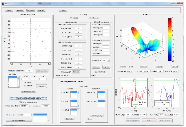
In order to test different configurations of the array for OTH radar, the tool Antenna Framework Simulator (AFS) has been implemented. The tool allows designing, visualizing and analyzing several planar array shapes, through dedicated GUIs. The AFS is very flexible.

Some GUIs for designing circular concentric arrays and spiral arrays are showed in Figure 2.1.

The array geometry chosen for OTH application is a circular shape and it consists of 50 radiating elements, like reported in Figure 2.2. The last choice is a compromise between a study made on the reduction of the mutual couplings (well explained in the following paragraph) between the elements and the radiation patterns of the phased array according to the frequency and the pointing direction. The radiation pattern of the phased array for OTH radar has to realize very low Side Lobe Levels.

Figure 2.1 – AFS GUI for spiral array design.

2.2 Stand alone antenna design for OTH array

As mentioned before, the configuration of the antenna thought for radar purposes has to be compact, but at the same time with broadband performances in the HF band.

We assume that the stand alone antenna has to operate in the range of 7MHz to 30MHz, with input impedance equal to 50Ω and it has to realize a maximum gain equal to 4dBi. The shape of the radiation pattern has to maintain the same shape according to the frequency and it has to be omni-directional on the H plane, and symmetrical on the E plane with a linear polarization.

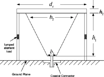
The first version of the antenna was a combination of a biconical antenna and a meandered antenna placed on a perfect electrical conductor infinite ground plane. It consists of two pieces, the nearest to the ground is similar to a conical antenna and the second one goes straight to a flat top.

The resulting antenna was formed of six folded arms and with one stub on the top (as shown in Figure 2.3). The height of the antenna was equal to 10.5m and the width was 6m and it was made of copper wires having a radius equal to 0.015m.

(a)

(b)

(a)

(b)

Figure 2.4 – Antenna first design radiation pattern: (a) E plane; (b) H plane.

The antenna performances have been analyzed with a Method of Moment (MoM) solver and it operated like a monopole on a perfect ground plane, with very good performances in terms of matching in the band of interest (Figure 2.3 (b)). At the same time, it presented good performances in terms of radiation pattern, however on the E plane the shape was quite different at higher frequencies than the lower frequencies one Figure 2.4. The antenna radiated with a linear polarization.

Because the proposed configuration was not physically feasible, another solution has been proposed, having the same performances but with a different shape. The new antenna consists of twelve arms joined together on the top Figure 2.5. This new configuration gives to the antenna more structural and mechanical stability than the previous one. The performances in terms of input impedance and radiation pattern of this new antenna are reported in Figure 2.7- Figure 2.8 and they have been evaluated with a MoM solver.

Figure 2.5 – Antenna with the modified design.

Figure 2.6 – Input impedance of the antenna with the modified design.

The antenna has a VSWR less than 3 in the range 7-30MHz. The new antenna is smaller than the previous one, its height is 6.5m and its width is equal to 4.6m. The material of the wires is copper and their radius is equal to 0.015m. It can be notice that the lower operating frequency is higher than the first version antenna one.

(a) (b)

Figure 2.8 – Antenna with the modified design radiation pattern at 7MHz: (a) E plane; (b) H plane.

The radiation patterns are more stable in shape according to the frequency.

2.3 Mutual coupling in phased arrays

The scanning performance of the array is generally determined by the element spacing, which is limited by the element size. For wideband antennas the operating band is very broad, making the electrical distance between the elements larger as the frequency increases. Ideally, less than λ/2 spacing is desired over the frequency band. When the element size is large, the spacing will easily exceed the λ/2 spacing at high frequency so the scanning performance of the array is degraded. However, if the distance between the radiating elements is reduced, mutual couplings phenomena are inevitable. The better solution is a continuous study of a trade-off between the two aspects: the stand alone broadband antenna and the antenna inside the array in the nearby of other identical elements.

The mutual coupling between the elements also depend on the shape of the array, the radiation pattern of the single element, on the frequency and the pointing direction [12], [13], [14].

The impedance matching of a standalone antenna is different and more complicated from the impedance matching of the same antenna inside the array.

The parameter which in a phased array takes into account all these variables is the active

reflection coefficient and its formulation for the m-th radiating element in the array is [14]:





0 0 0

sin ( )cos ( )sin

sin ( )cos ( )sin

0 0 0, 1 0, , | | mn jk x m y m N j S jk x n y n m mn n n m e S e V e V               



  ₀, ₀ indicate the generic pointing direction,

 V_0,i is the voltage feeding of the generic radiating element i,  x(i), y(i) are the coordinates of the generic element i,

 S is the scattering matrix at a generic frequency f,  k2 /  is the wave number.

If we consider constant source amplitude for each element in the array, the active

reflection coefficient can be written as follow:





0 0 1, , N jk x m y m jk x n y n m mm mn n n m S e    S e             



In order o reduce the mutual coupling in a phased array, the active reflection coefficient

Γm has to be minimized.

The parameter Smm is the active reflection coefficient of the m-th element fed and the

other elements terminated on 50Ω. The last term is the only one of the sum which is independent from the frequency. The second term of the sum is frequency dependent. Because all the terms Smn are generally lower than the term Smm, the active reflection coefficient can be

minimized if the term Smm is minimized. This last assumption is necessary in order to

minimize Γm, but not sufficient, because sometime it can happen that a coherent summation of

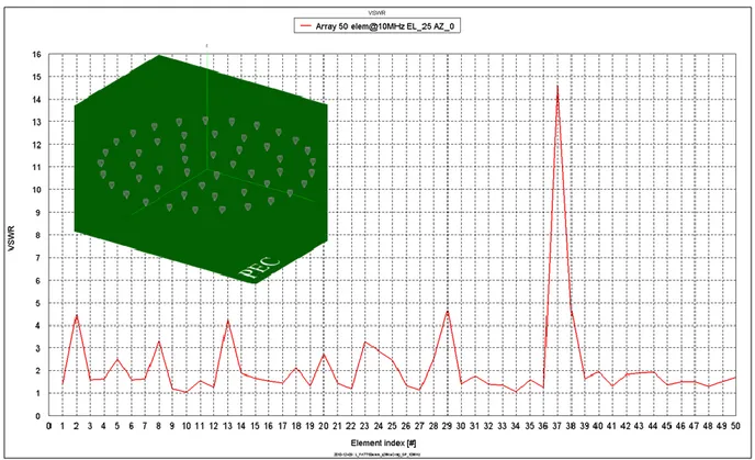
In Figure 2.9 an active VSWR of a circular phased array of 50 elements has been reported, in order to show how even if the antenna are broadband well-matched, the mutual coupling creates a mis-match of the entire array.

Figure 2.9 – Active VSWR of a circular phased array according to the element inside the array.

Because each radiating elements in practice, is used with amplifiers, which support a VSWR at maximum equal to 3, the active VSWR realized by each element in the array doesn’t must exceed 3, and the active reflection coefficient doesn’t must exceed the value 0.5. Further, it is necessary that especially at lower frequencies of the HF band used for OTH radar purposes (8-16MHz at least), the generic m antenna in the array has to realize the Smm as small

as possible.

We took into account all these requirements for the study of the stand alone antenna, which has been explained in the following paragraphs.

2.4 Miniaturizing the stand alone antenna

In order to reduce the mutual couplings coming from the use of the antenna in the array, a modified configuration has been studied into respect the two versions presented before (§2.2).

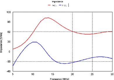
By observing the imaginary part of the input impedance of the original antenna according to the frequency, an inductive behaviour can be notice in the range 7.3MHz-13.27MHz, otherwise the antenna has got a capacitive behaviour.

(a) (b)

Figure 2.10 – Antenna input impedance: (a) RE (Zin); (b)IM (Zin).

Two different approaches have been studied and compared with the original antenna case: the first one by using a folded pin [17] near the antenna and the second one by using a coupled pin [18]. The first pin has been used because of its inductive behaviour, in order to compensate the capacitive behaviour of the input impedance of the antenna at lower frequencies of the HF band (as shown in Figure 2.11). The second pin behaves as a capacitance and it could compensate the inductive behaviour of the antenna in the range 7.3MHz-13.27MHz.

At the same time, the new configuration has to match the real part of the antenna to 50Ω. In the here proposed configurations only the antenna was fed and not the pin.

Both cases have widely been studied with a parameterization of the segments constituting the pins. For the optimization, the input impedance and the VSWR of the antenna have been taken into account.

(a)

(b)

2.4.1 Antenna with inductive pin: matching

For the folded pin case (Figure 2.11 (a)), the lengths of the segments have been investigated and the VSWR has been observed.

First of all we fixed the length of the segments e, d and g equal to 1m and we varied f, b and a.

(a)

(b)

Figure 2.12 – Antenna with folded pin: (a) segments parameterization; (b) VSWR parameter according to the frequency and parameters b and f.

As it can be seen from VSWR (Figure 2.12 (b)), a very good matching of the antenna at the lower frequencies of the HF band, has been obtained.

The solution with b and f equal to 0.5m has been considered for further investigations, because it realizes the better VSWR performances.

Then, fixing f and b equal to 0.5m, we varied the length of the segments d and g, studying the behaviour of the antenna with three different values of the segment e (Figure 2.13 - Figure 2.15).

(a)

(b)

Figure 2.13 – Antenna with folded pin: (a) segments parameterization; (b) VSWR parameter according to the frequency and parameters d and g.

(a)

(b)

Figure 2.14 – Antenna with folded pin: (a) segments parameterization; (b) VSWR parameter according to the frequency and parameters d and g.

(a)

(b)

Figure 2.15 – Antenna with folded pin: (a) segments parameterization; (b) VSWR parameter according to the frequency and parameters d and g.

We observed that good performances have been obtained in the case of d and g equal to 1m.

2.4.2 Antenna with inductive coupled pin: matching

While the introduction of the simple folded pin, as described in the previous paragraph, produced a capacitive load for the antenna, which compensates the inductive behaviour of the antenna especially in the range 7.3-13.27MHz, after the introduction of a further grounded pin, we noticed a compensation of the capacitive behaviour of the antenna in the center of the considered band.

So we investigated the performance of the antenna according the width of the gap, which operates like an inductive load. At the beginning we chose a width of the gap, as the segment e equal to 1m and then we fixed the gap and the segment e to 0.2m. Thus we compared the results between the antenna loaded with original folded pin and with the unloaded antenna.

Figure 2.16 – Antenna with folded coupled pin.

(c)

Figure 2.17 – Antenna with folded coupled pin: (a) RE(Zin) according to the frequency; (b) IM(Zin) according to the frequency; (c) VSWR according to the frequency.

A good matching has been obtained until 18MHz. At higher frequencies, the effect was not so significant.

According to the latter observations, we studied the combination of the folded coupled pin and the simple one, by varying the gap between the antenna and the pin as follows.

(a)

(b)

(c)

Figure 2.19 – Antenna with folded coupled pin: (a) RE(Zin) according to the frequency; (b) IM(Zin) according to the frequency; (c) VSWR according to the frequency.

By using a much closed grounded pin to the antenna, the coupling was stronger especially in the center frequencies of the band. The last transformation causes more

oscillations of the input impedance, leading to an overall improvement of the matching. However the effect of the reduction of the gap was no significant at lower frequencies of the HF band, so a further study was required.

We thought to introduce other conductive paths to the original pin in order to enhance its inductive behaviour. As it can be seen in Figure 2.20, we added a new path parallel to the existent path i, having the same length of i.

Figure 2.20 – Antenna with folded coupled pin with a further path parallel to i.

In the following Figure 2.21, the results in terms of input impedance and VSWR have been shown. The introduction of the segment parallel to i produced a better matching of the antenna, especially at lower frequency and further the positive effect is present also at other frequencies.

(a) (b)

(c)

Figure 2.21 – Antenna with folded coupled pin and a further segment parallel to i: (a) RE(Zin) according to the frequency; (b) IM(Zin) according to the frequency; (c) VSWR according to the frequency.

Finally, the best performances in terms of matching for our purposes have been obtained with the last solution, which takes into account the combination of a simple folded pin, together with a path coupling the antenna with a very small gap and finally, having a further vertical path.

In the last results we didn’t show the performances of the new solution of the antenna in terms of radiation pattern. They are very important, especially in radar application, in which specifics radiation patterns on the principal planes have to be realized. They are showed in the following paragraph.

2.4.3 Antenna with folded coupled optimized pin: radiation pattern

The antenna with different type of the folded pin presents a very good matching, and the target of a very good matching at lower frequencies was obtained. Together with the matching analysis, the radiation pattern of the antenna has been observed according to the frequency, and on the principal planes: E plane at phi=0° and E plane at phi=90°, which coincide with the

xz plane and the yz plane respectively and H plane, which coincides with the xy plane.

(a)

(b)

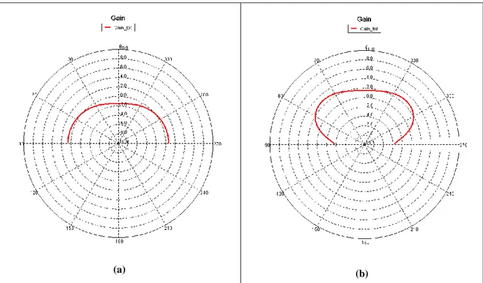
Figure 2.22 – Antenna with folded coupled optimized pin tri-dimensional radiation pattern: (a) 14MHz; (b) 17MHz.

(a) (b)

Figure 2.23 – Antenna with folded coupled optimized pin radiation pattern, phi=0°: (a) 14MHz; (b) 17MHz.

(a) _(b)

Figure 2.24 – Antenna with folded coupled optimized pin radiation pattern, phi=90°: (a) 14MHz; (b) 17MHz.

(a) (b)

Figure 2.25 – Antenna with folded coupled optimized pin radiation pattern, H plane: (a) 14MHz; (b) 17MHz.

The radiation pattern on the H plane was no more omni-directional and no more symmetrical on the E plane, especially for some frequencies, as it can be seen in Figure 2.25. In some cases, it presented many differences between two closed frequencies.

In Figure 2.23 to Figure 2.25 the radiation patterns at 14MHz and 17MHz are shown respectively. The radiation pattern of the antenna at these latter frequencies in fact, differs so much.

The target on the radiation characteristics of the antenna was lost with the use of a single folded pin because the antenna is no more electrically small. We needed to reduce its size in order to maintain the symmetry of the radiation pattern on the E plane, and the omni-directional behaviour on the H plane.

2.4.4 Antenna with folded coupled optimized pin: miniaturization

The antenna with the folded coupled optimized pin has been miniaturized in two different ways. First, we applied a factor equal to 0.5 to all the original sizes of the antenna,

and then we reduced the size in order to reach all the sizes contained on a sphere having the radius compliant with the Wheeler limit [6] at the central frequency of the band. For the latter reason we chose a radius equal to 3x3x3 m3. Actually, according to the Wheeler limit, the antenna should be contained in the sphere having radius equal to 1/k. In our case the segment c is not exactly contained in that radius, nevertheless we decided to use it because it is a key point for the antenna matching.

Figure 2.26 – Antenna miniaturized design.

Table 2.1 – Size description of the miniaturized antennas. Feed, p [m] h 1 [m] h 2 [m] R 1 [m] R 2 [m] a [m] b,f [m] c [m] d,g [m] e, gap [m] n [m] Original 0.1 2.5 3.9 0.23 2.07 4 2.5 2 1 0.2 4.41 Miniaturized (Factor 0.5) 0.1 1.25 1.95 0.115 1.035 2.05 1.25 1 0.5 0.1 2.21 Miniaturized (3x3x3) 0.1 1.9 1 0.1 1.4 2.1 1 1 0.5 0.1 2.44

Table 2.2 – Size comparison between the original and the miniaturized version of the antenna. Height [m] Width [m] Original 6.5 4.6 Miniaturized (Factor 0.5) 3.3 2.3 Miniaturized (3x3x3) 3 3

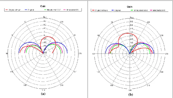
In the following Figure 2.27, we showed the results obtained with the size reduction, and we compared the results between the original antenna, the antenna with the folded coupled pin and finally the two versions of the miniaturized antenna.

(a) _(b)

(c) (d)

Figure 2.27 – Antenna and its miniaturization versions comparison: (a) RE(Zin) according to the frequency; (b) IM(Zin) according to the frequency; (c) VSWR according to the frequency; (d) S11 in dB

according to the frequency.

In terms of matching, by observing the S11 in dB, the miniaturized antenna with a factor equal to 0.5 had very good performance for frequencies in the range 13-21.07MHz. At lower frequencies it is mismatched and at higher frequencies it presents a worst matching than the original antenna. The miniaturized antenna with the use of the Wheeler limit had good performances up to 13.86MHz and the matching is always better than the original one; however it is mismatched at lower frequencies. In both cases, the mismatching is due to the

fact that the size of the antennas at lower frequencies is very small compared to the wavelength, and it behaves like an ideal dipole (e.g. at 5MHz its size is around 0.05λ) [16]. The same behaviour can be noticed by observing the real impedance at these frequencies, which is very low (few Ohms) compared to the values obtained at other frequencies. For the latter reasons the proposed antennas could only be used for our purposes in the higher part of the HF band.

It can be notice that by using a miniaturized version of the antenna with the pin, we reached again the symmetry on the radiation pattern on the E plane q.e.d. (Figure 2.29- Figure 2.30). The radiation pattern is again omni-directional on the H plane (Figure 2.31); however a decrease of the maximum gain of the antenna is inevitable, because the antenna has got smaller size than the original one.

The shape of the radiation pattern according to the frequency is almost the same.

(a) _(b)

Figure 2.28 – Antenna with folded coupled optimized pin miniaturized (0.5 factor) tri-dimensional radiation pattern: (a) 14MHz; (b) 17MHz.

(a) _(b)

Figure 2.29 – Antenna with folded coupled optimized pin radiation pattern, phi=0°: (a) 14MHz; (b) 17MHz.

(a) (b)

Figure 2.30 – Antenna with folded coupled optimized pin radiation pattern, phi=90°: (a) 14MHz; (b) 17MHz.

(a)

(b)

Figure 2.31 – Antenna with folded coupled optimized pin radiation pattern, H plane: (a) 14MHz; (b) 17MHz.

In Table 2.3 we compared the maximum gain of the original antenna, with the maximum gain obtained with the two miniaturized versions. With the reduction of the size of the antenna, we reached again the performances on the shape of the radiation pattern, but we lose in terms of the gain, especially if we consider the 3x3x3m3 version of the antenna.

Table 2.3 – Gain comparison between the original and the miniaturized versions of the antenna. Maximum gain @ 14MHz [dB] Maximum gain @ 17MHz [dB] Original _{3.72 3.63} Miniaturized (Factor 0.5) 1.0 2.2 Miniaturized (3x3x3) 0.23 1.43

We can conclude that both the miniaturized antennas don’t cover the whole frequency range in the HF band, but just the higher frequencies. For our purpose, the last solution obtained is far from the specifics of OTH radar.

Figure 2.32 – VSWR of the 0.5 factor miniaturized antenna according to the frequency.

However, it should be noted that the two miniaturized antennas are capable of operating over a very wideband in the range 13-90MHz (Figure 2.32), and then they can be proposed for VHF applications.

For phased array radar application, we have to use another kind of solution, like e.g. some matching networks, which can realize very good matching at single frequencies (narrowband matching) or on a wide range of frequencies (wide band matching network). The theory and performances of different matching networks have been widely investigated in the following chapter.

3 I

M

N

In the previous chapters, we showed how the mutual coupling is strong at lower frequencies of HF band. For OTH radar array purposes, the lower frequencies are important because they allow covering high distances in space with respect to the radar site.

Several stand alone antenna configurations have been investigated. The stand alone original antenna doesn’t allow reaching very good performances at lower frequencies, where the mutual coupling is strongest. So, other configurations, with inductive pins causing the capacitance compensation have been studied. However, a miniaturization is required, in order to maintain the performances of the antenna in terms of radiation pattern. The miniaturized version realizes a translation of the operating bandwidth of the antenna. In order to compensate the capacitive behaviour of the antenna, the use of impedance matching network is inevitable.

Further, as mentioned in §2.3, the stand alone antenna has to realize a VSWR as small as possible. All the presented radiating elements respect the constraint on the VSWR<3, which corresponds to a S11<-6dB. The last constraints for the phased radar array are not good enough, because the mutual couplings.

For these reasons, we rearranged the specifics on the stand alone antenna matching, making them stricter. The stand alone antenna has to be realize an S11<-17dB in the range 8-21MHz, where the mutual couplings are stronger; a S11<-6dB are enough for higher frequencies (21-30MHz), where the mutual coupling is less strong.

In order to reach those performances, the antenna used with the matching networks is 0.5m higher than the antenna presented in previous chapters and it consists of 18 arms and the radius of the wires is equal to 0.020m. This antenna configuration presents better impedance matching performance than the previous one, especially in the centre of the HF band.

The Figure 3.1 shows the active VSWR of the new antenna in the circular phased array of 50 elements at 12MHz, according to the pointing direction of the beam.

Figure 3.1 – Active VSWR of the circular phased array at 12MHz.

A narrowband matching network has been designed for the stand alone antenna and then it has been used for each element (Figure 3.2) of the circular array reported in Chapter 2.

Figure 3.2 – Narrowband matching network of each radiating element of the circular phased array.

The vantage of the use of a very well-matched antenna in the array is showed in Figure 3.3: it can be notice that the mutual coupling is less strong.

Figure 3.3 – Active VSWR of the circular phased array at 12MHz: each element matched with a narrowband matching network.

Because the interest is to reduce the mutual coupling also according to the frequency, let assume that the number of frequencies of interest are equal to M and the number of the elements of the phased array are N, with A and φ the amplitude and the phase of the sources respectively.

(a)

(b)

Figure 3.4 – Matching networks in the phased array: (a) use of MxN narrowband networks; (b) use of M wide-band matching networks.

Thus, two possible approaches of the use of matching networks have been thought and investigated:

1. the use of MxN narrowband matching networks (Figure 3.4 (a)), 2. the use of N wideband matching networks (Figure 3.4 (b)).

The first approach can be useful in the case in which the transmission of the radar signal is made with a discrete occupation of the frequencies in the range 8-30MHz.

The second approach can be fit with the need of a continuous occupation of the frequencies in the range 8-30MHz.

At the beginning, according to literature a several number of matching networks topologies have been designed. After that, we provide a new methodology in order to obtain good compromise in terms of bandwidth, combining the analytical design with optimization algorithms.

3.1 Narrowband impedance matching networks

The performance of an impedance matching network depends on the factor of quality Q, inversely proportional to the operating bandwidth. A network designed with a high Q factor is a narrowband network; otherwise small Q values imply wideband networks. Different topologies are used in literature in order to realize the matching, and they depend on the number of the lumped element used. For the purposes of this work, we avoid to use resistances in the matching network, in order to maximize the efficiency of the antenna, reducing the losses. An L topology matching network allows obtaining a good matching at a specified frequency with just two elements, like the combination of a capacitance and an inductance. Instead, the T and π topologies allow obtaining the matching with three lumped elements, as a combination of capacitance and inductance as well.

3.1.1 L topology matching network

With L topology matching network is possible to reach the matching with the maximum factor Q achievable with a matching network. However, because the Q factor depends on the impedance of the load and the impedance of the source, it is fixed and it cannot be modified.

For the design of an L network, in literature there is a specific criterion, just by knowing the impedance of the load RL, the impedance of the source Rs and the frequency [24].

Figure 3.5 – Several combinations of L-matching networks. In (a)–(c) the load is connected in series with the reactance boosting the input resistance. In (d)–(f) the load is in shunt with the reactance,

lowering the input resistance.

Let R_max max(R R_S, _L) andR_min min(R R_S, _L), the L-networks shown in Figure 3.5 are designed as follows:

1. Calculate the factormRmax Rmin_.

2. Compute the required circuitQ m1.

3. Choose the topologies from Figure 3.5(a)-(c) if you are boosting the resistance, i.e. RS>RL, thenXs  Q RL. If you are dropping the resistance, i.e. RS<RL, choose

(d)-(f), thenX_p R Q_L .

4. Compute the effective resonating reactance. If RS>RL, calculate Xs' Xs(1 Q 2) 

 

and set the shunt reactance in order to resonate, '

p s

X  X . If RS<RL, then

calculate ' ₍₁ 2₎

p p

X  X Q and set the series reactance in order to resonate,

'

s p

X  X .

5. For a given frequency of operation, pick the value of L and C to satisfy these equations as follows: L X/ andC1/X .

Actually, in the most of the cases the impedance of the load has a reactance part, e.g. RL±jXL, which has to be compensated, in order to reach the matching. This behaviour is found

There are two basic approaches in handling complex impedances [23]:

1. Absorption: To actually absorb any stray reactance into the impedance-matching network itself. This can be done through prudent placement of each matching element such that element capacitors are placed in parallel with stray capacitances, and element inductors are placed in series with any stray inductances. The stray component values are then subtracted from the calculated element values, leaving new element values (C’, L’), which are smaller than the calculated element values.

2. Resonance: To make resonant any stray reactance with an equal and opposite reactance at the frequency of interest (Figure 3.6).

For our purposes we will use the resonance approach.

Figure 3.6 – L-network: Resonance approach.

Most of the cases, during the design of an impedance matching network, both the techniques are used. However, if the stray element values are larger than the calculated element values, absorption cannot take place. In a situation such as this, when absorption is not possible, the concept of resonance coupled with absorption will often do the trick. The two methods presented are valid also for T or π matching networks design.

Sometime it is easier to implement some known formulas, present in literature, which take into account the complex load characteristic. There are eight combinations of L and C (shown in Figure 3.7) in order to cover all complex loads on the Smith chart [20].

Figure 3.7 –Yin-Yang regions on the Smith chart for L-matching networks design.

Each green zone describes a region of impedances on the Smith chart (Yin-Yang region) which can be matched with the correspondent LC-network combination.

Let Z_L R_L jX_L

,, the load impedance, and Rs, the source impedance, it can be possible to choose one of the eight combinations (Figure 3.7) which perfectly match the load to the source and to calculate the values of each components with the formulas described in Appendix A.

3.1.2 T and π topologies matching networks

With T and π topologies matching network is possible to reach a narrowband matching because the Q factor depends on the virtual resistance, on the source and the impedance of the load, so it is controllable.

The π topologies matching network are designed with three lumped elements, shaped as a pi-greco. They can best be described as two “front-to-front” L networks that are both configured to match the load and the source to an invisible or “virtual” resistance located at the junction between the two networks, as shown in Figure 3.8.

Figure 3.8 – π - network designed as two front-to-front L topologies.

The significance of the negative signs for −Xs1 and −Xs2 is symbolic. They are used merely to indicate that the Xs values are the opposite type of reactance from Xp1 and Xp2, respectively. Thus, if Xp1 is a capacitor, Xs1 must be an inductor, and vice versa. Similarly, if Xp2 is an inductor, Xs2 must be a capacitor, and vice versa. They do not indicate negative reactances (capacitors).

The virtual resistance (R) must be smaller than either Rs or RL because it is connected to the series arm of each L section but, otherwise, it can be any value you wish. Most of the time, however, R is defined by the desired loaded Q of the circuit that you specify at the beginning of the design process. For our purposes, the loaded Q of this network will be defined as:

max ₁

R Q

R

  (3.1)

whereRmax max(R RS, L)_{. Although this is not entirely accurate, it is a widely accepted}

Proceeding from the load to the source, further it is necessary to define QL e QS, which

are the quality factor of the first L-network and the second L-network respectively. They are defined as follows: 1 1 L L S S R Q R R Q R     (3.2)

Assuming a total quality factor equal to Q and described as in (3.3), from (3.3) it can be possible to get the virtual resistance R from the inverse formulation, as follows:

max 2 1 R R Q   (3.3)

Finally, the reactances of the π-network are described as:

1 , 1 , 2 , 2 S L p s S s L p S L R R X X RQ X RQ X Q Q     (3.4)

In the design of a π-network, it must be defined the subsequent quantities:

max min min min 1 , min( _S, _L) R Q R R R R    (3.5)

In order to verify these conditions [22]:

min min

QQ  R R (3.6)

So, the Q factor of a π-network is always maximum than Qmin, i.e. the minimum Q

factor, just realizable with a single L matching network.

The T topologies matching network are designed with three lumped elements, shaped as a “T” (Figure 3.9). They can best be described as two “back-to-back” L networks. The load and the source are matched through these two L-type networks, to a virtual resistance that is