Preliminary stages and studies for the development of a 3D aquifer physical model

(1)

ALMA MATER STUDIORUM – UNIVERSITY OF BOLOGNA

SCHOOL

OF

ENGINEERING

AND

ARCHITECTURE

DICAM

Department of Civil, Chemical, Environmental and Materials Engineering

Master Degree : Environmental Engineering Curriculum : ERE, Earth Resources Engineering

Master Thesis of

Groundwater Quality, Protection and Modelling

Preliminary stages and studies for the development of a

3D aquifer physical model

CANDIDATE PROMOTOR ULG

Laura Balzani Prof. Serge Brouyère

CO-PROMOTOR UNIBO Prof. Lisa Borgatti

Academic Year 2018/19 Session II - 3 OCTOBER 2019

(2)

Within a Dual Degree programme with Alma Mater Studiorum

University of Liège

Master of Environmental Earth and Resource Engineering

« Ingénieur civil des mines et géologue, à finalité spécialisée en géologie de l'ingénieur et de

Preliminary stages and studies for the development

of a 3D aquifer physical model

Student : Laura BALZANI

1

ULiège – UNIVERSITY OF LIEGE Within a Dual Degree programme with Alma Mater Studiorum - UNIVERSITY OF BOLOGNA

Liège - Faculty of Applied Sciences – Department ARGEnCo Academic Year 2018 - 2019

Master of Environmental Earth and Resource Engineering

Ingénieur civil des mines et géologue, à finalité spécialisée en géologie de l'ingénieur et de l'environnement »

Master Thesis

stages and studies for the development

of a 3D aquifer physical model

Prof. Serge BROUYÈRE

Prof. Lisa BORGATTI (UNIBO)

Members of the Jury: Serge BROUYÈRE Alain DASSARGUES

Sébastien

UNIVERSITY OF BOLOGNA

ARGEnCo

Ingénieur civil des mines et géologue, à finalité spécialisée en géologie de l'ingénieur et de

stages and studies for the development

Promotor: Serge BROUYÈRE (ULG)

Co-Promotor: Prof. Lisa BORGATTI (UNIBO)

Members of the Jury: Serge BROUYÈRE Alain DASSARGUES

(3)

(4)

3

Abstract

Groundwater issues are among the most important sustainability studies related to topics considered as critical point for the future of planet Earth (Gleeson et al., 2010) in the perspective of a sustainable world. Analyses are focused on two complementary aspects: quantity and quality. Thus, once physical behaviour is analysed, it is coupled with chemical characterisation studies, in order to obtain a better view of an investigated site. The work of this Master thesis begins with a brief overview of the literature which summarizes the challenges of teaching hydrogeology by theoretical lessons coupled with practical activities. The focus is on laboratory experiments implemented on physical models. In fact, to fully understand the process of groundwater flow and solute transport, and to demonstrate the basics fundamental concepts behind, it is important to visualize them in a lab-scale. This thesis is undertaken in the context of the installation of a 3D physical model at the University of Liège as a support to teaching and research works: dimension, set up, construction and support devices used for system optimal functioning are presented. The global aim of the work is to prepare everything needed to set up the sand tank. This is a fundamental step in order to be able to pre-dimension real experiments, to give ideas about the magnitude order of the expected results and to check the reliability of mathematical results and/or low-dimensionality models. Part of the document is centred on the characterization of porous aquifer materials to implement in the physical model, in particular through sand column one-dimensional lab experiments performed on four distinguished types of quartz sands (differentiated by the particles size): in particular a Constant Head Permeability Test and a Salt Tracer Test (KCl). A numerical model of the 3D tank is also developed by the use of GMS-MODFLOW-MT3DS and few experiments are simulated (gradient variation, pumping test at different pumping rates, and tracer test).

(5)

(6)

5

List of Figures

FIG 1 Integrated hydrogeology pedagogy associated to an iterative loop over three class components. Within this iterative loop, each component supports the others with chains of mutual feedback. Inspired from Gleeson

et al. (2012) and Hakoun et al. (2013). ... 24

FIG 2 Aquifer model constructed by students for the groundwater remediation lab activity (Hilton, 2008) ... 25

FIG 3 Apparatus for hydraulic conductivity determination: Falling head test (Nicholl et al., 2016) ... 27

FIG 4 Experimental setup of Constant-head test (black) and Tracer test (black and blue) (Cai et al., 2015) ... 27

FIG 5 Physical 2D model of an aquifer: scheme + real example (sources : Lane, Guide to Sand tank, and https://etc.usf.edu/clippix/picture/front-view-of-the-groundwater-model.html, consulted in July 2019) ... 29

FIG 6 Experimental sandbox set up (Jose et al. 2004) ... 30

FIG 7 Lab-scale flow tank: A-Colloidal borescope (Wu et al. 2008) and B-Monitoring well (Verreydt et al. 2015) ... 32

FIG 8 Darcy’s Law (source: PPT Permeability in soils, Geotechnical Lab, Civil Eng Texas University) ... 36

FIG 9 Dimensions and pictures of the sandbox developed at ULiège ... 44

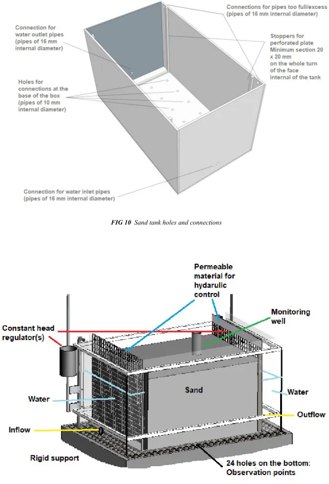
FIG 10 Sand tank holes and connections ... 46

FIG 11 Components view of the sand tank (modified from iFLUX, 2018) ... 46

FIG 12 Mariotte Bottle used to keep and provide constant hydraulic head (Nicholl et al.2016) ... 48

FIG 13 Constant head open overflow devices ... 48

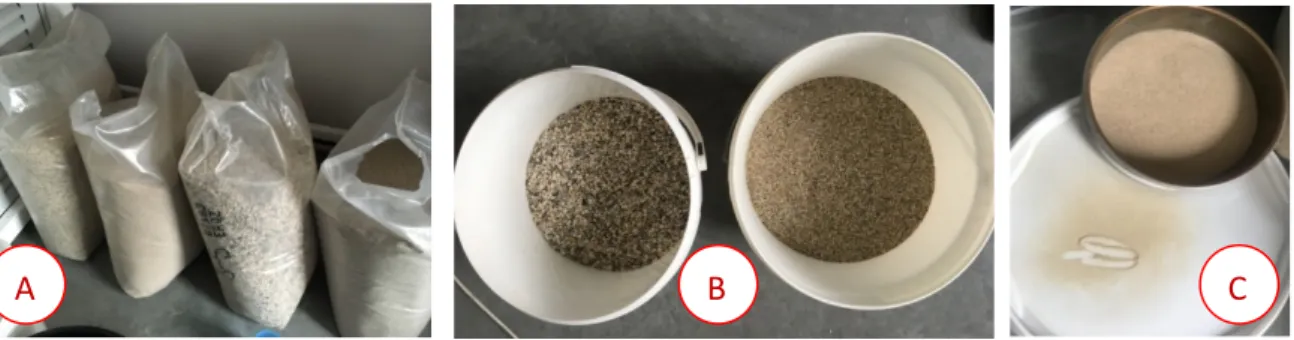
FIG 14 Available type of sands to characterize through column experiments (A,B) and impurities check by sieving (C) ... 50

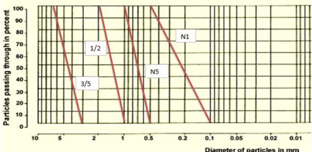
FIG 15 Granulometric Curve to determine geotechnical parameters of all studied sands ... 51

FIG 16 A) Soil type analysis: graph to estimate a priori total and effective porosities, with retention capacity; and B) Aquifer analysis (Eckis, 1934 modified) ... 51

FIG 17 Schematic diagram of experimental equipment for tracer test in soil column (Ujfaludi, 2010) ... 53

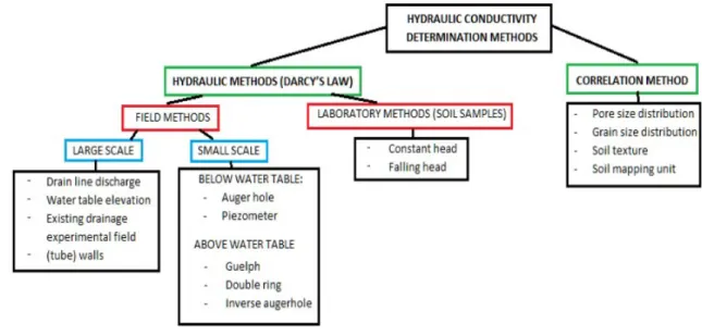
FIG 18 Overview of methods for the hydraulic conductivity determination (Ritzema 2006) ... 54

FIG 19 Constant head permeameter (Domenico and Schwartz 1990) ... 55

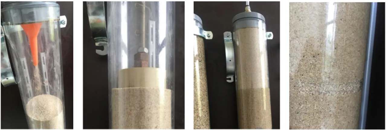
FIG 20 Funnel use, compaction, saturation and observation of the final columns preparation ... 58

FIG 21 Metallic plate to apply to the filter ... 59

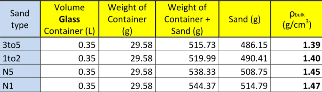
FIG 22 Bulk density lab evaluation ... 62

FIG 23 Schematization of the packing of spherical grains and possible pore size (Říha et al., 2018) ... 65

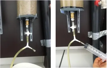
FIG 24 Final constant head set up : A schema and B real system used ... 71

FIG 25 Falling head operational scheme ... 73

FIG 26 Statistics on N1 empirical K-values (all formulas) ... 76

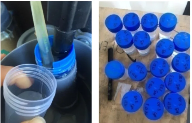
FIG 27 Brief injection of tracer: syringe manually pressed ... 78

FIG 28 Probe to monitor the EC-values, and water sampling during tracer test ... 79

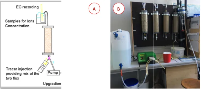
FIG 29 Implementation of tracer test: A) the scheme and B) the practical set up ... 80

FIG 30 Pre-dimensioning of the KCl tracer test for sand-columns: A) Infinite and B) Semi-infinite (selected) .... 81

FIG 31 Correspondence of EC values (Probe vs Lab analysis): sand 1to2 (A) and N1 first test (B) ... 82

FIG 32 EC-Curves comparison between lab and probe measurments after injection: test1 N1sand (A) and test5 3to5sand (B) ... 83

FIG 33 Ion concentration: comparison Cl- and K+ breakthrough curves (sand N1, second test)... 84

FIG 34 Linear correspondence between EC and concentration[K+]: case of sand 1to2 (A;C-EC,Lab vs mg/L, mmol/L; B;D-EC,Probe vs mg/L, mmol/L) ... 85

FIG 35 Linear correspondence between EC and concentration[Cl-]: case of sand 3to5 (A;C-EC,Lab vs mg/L, mmol/L; B;D-EC,Probe vs mg/L, mmol/L) ... 86

FIG 36 BTCs normalized comparison between the different sand samples ... 87

FIG 37 Interpretation of breakthrough curve of Cl- ions concentration (mg/L) in 1to2 sand ... 89

FIG 38 Interpretation of breakthrough curve of Cl- ions concentration (mg/L) in N1 sand (second test) ... 89

FIG 39 BCs of FLOW numerical model of physical 3D sand tank ... 93

FIG 40 Conceptual model implementation through coverages in GMS ... 95

FIG 41 Tracer injection model coverage visualisation (without grid) in GMS ... 97

FIG 42 Steady state flow (Δh = 7 cm): lateral and top view, grid visualization ... 100

FIG 43 Graph showing the different phases of a constant rate (British Columbia, 2007) ... 102

(11)

10

FIG 45 Step test implemented ... 103

FIG 46 Step pumping test: heads variation ... 104

FIG 47 Step pumping test: Drawdown variations ... 104

FIG 48 Step pumping test: water table variation passing from Q2 to Q3 ... 105

FIG 49 Examples of results associated to brief and continuous injection breakthrough curves numerically obtained ... 107

FIG 50 Comparison BTCs continuous tracer inj (A-MOC, B-TVD, C-Comparison) correcting the value of the dispersivity ... 108

FIG 51 Continuous tracer injection with MOC and TVD advection solution (plume comparison at min 25,red background corresponding to zero concentration) ... 109

FIG 52 BTCs continuous injection simulated applying increment in prescribed Δh (MOC solution used) ... 110

FIG 53 Change in water surface in relation to variations of K (m/s) ... 111

FIG 54 Head comparison while varying K value (A for KN5, B for K3to5) ... 112

FIG 55 BTCs for Continuous tracer injection MOC (changes in neff and αL)... 114

FIG 56 BTCs for Brief tracer injection, MOC solution, and changes in neff) ... 114

FIG 57 Different examples of 2D physical aquifer model: landfill presence and different geological structures (https://www.realscienceinnovations.com/groundwater-models.html, consulted in April 2019) ... 117

FIG 58 Sand aquifer for classroom demonstrations and example of streamflow generation (A-Silliman et Simpson, 1987; and B-C- Rodhe 2012) ... 117

FIG 59 Cell and its interfaces identification: Standard finite-difference method (MT3DMS Manual, 1999) ... 118

FIG 60 TVD schema of operation (Dassargues, 2019) ... 119

FIG 61 Illustration of the method of characteristics (MT3DMS Manual, 1999) ... 120

FIG 62 Filters bottom of the column: porous disks, net (4 layers to have a more consistent strata- grey in the figure), very permeable sponge material (black in the figure) ... 122

FIG 63 Top of the column: little stones used to keep the sands unable to go out from the system during the experiments ... 122

FIG 64 On left side it is shown the column preparation: first layer of water and then sand added; On the right picture the final four columns of the first trial is presented ... 123

FIG 65 Preferential paths visualization and similar correlated problems ... 123

FIG 66 Sand N1 escaping the system while applying water circulation ... 124

FIG 67 Air bubbles and channels not filled by water in the finer sand samples plus bubbles of air entering the system together with water ... 124

FIG 68 Improvement of second and third trial in column preparation: changes in upper filters and hammer use to help air to exit ... 124

FIG 69 Problem of the second trial: still air bubbles trapped and sands exiting the system ... 125

FIG 70 Third trial characteristics (filters details) ... 126

FIG 71 Statistics on N5 empirical K-values (all formulas) ... 132

FIG 72 Statistics on N5 empirical K-values (selection of representative results) ... 133

FIG 73 Statistics on 1to2 empirical K-values (all formulas) ... 134

FIG 74 Statistics on 1to2 empirical K-values (selection of representative results) ... 135

FIG 75 Statistics on 3to5 empirical K-values (all formulas) ... 136

FIG 76 Statistics on 3to5 empirical K-values (selection of representative results) ... 137

FIG 77 Seven Layers model: central lateral section of water heads, while applying Qpump = 6.5x10-5 m3/s ... 142

FIG 78 Seven Layers model: drawdown while applying Qpump = 6.5x10-5 m3/s ... 143

FIG 79 Seven Layers model: central lateral section of water heads, while applying Qpump = 1x10-4 m3/s ... 143

FIG 80 Seven Layers model: water head and relative drawdown, while applying Qpump = 1x10-4 m3/s ... 144

FIG 81 Seven Layers model: central lateral section, while applying Qpump = 2.5x10-4 m3/s ... 144

FIG 82 BTCs for Continuous tracer injection TVD (changes in neff and αL) ... 145

(12)

11

List of Tables

TABLE 1 British Soil Standard Classification of Sandy soil ... 49

TABLE 2 Geotechnical parameters estimated for the four types of sand studied ... 50

TABLE 3 Expected and estimated ranges for sands parameters to be determined ... 51

TABLE 4 Summary of columns preliminary measurements ... 61

TABLE 5 Results of bulk dry densities evaluation for all the four types of sands studied with glass experiment . 63 TABLE 6 Results of bulk densities for all sands studied through column samples ... 63

TABLE 7 Total porosity of all types of sand studied ... 64

TABLE 8 Results of analytical computation (Terzaghi K as the closest to the experimental ones; range of variation) ... 68

TABLE 9 K-values calculated experimentally for each sand sample with CH test (range of variability min-max in green) ... 72

TABLE 10 Data of injections on different samples ... 78

TABLE 11 Tracer tests summary of analysis on first tracer arrival and peak time ... 87

TABLE 12 Summary of estimated parameters by the use of TRAC for all sands tested ... 90

TABLE 13 Packages implemented in MODFLOW for the flow model ... 96

TABLE 14 Flow (MODFLOW) and Transport (MT3DS) simulation solver characteristics ... 98

TABLE 15 Results of steady state flow simulations ... 99

TABLE 16 Step pumping test: influence radius and drawdown for higher pumping rate ... 106

TABLE 17 Different pumping rates applied on the 2 Layer Numerical Model ... 106

TABLE 18 Results of main ideal tracer tests with N5 sand ... 109

TABLE 19 Comparison of results of constant pumping rate test due to changes in K value ... 111

TABLE 20 Constant Inputs of empirical formulas (source: https://www.engineersedge.com consulted in April 2019) ... 127

TABLE 21 Summary of all empirical computation formulas and results ... 128

TABLE 22 Average K values from CHPT ... 129

(13)

(14)

13

Nomenclature

a Cross sectional area of the water level monitoring device (m2) A Areal section of the column (m2)

b Aquifer thickness (m)

B,C,D,E Linear coefficients/numbers used to make relations between variables (/) Cv Volumetric concentration of solute (kg/m3)

Cv*_{Volumetric concentration at intermediate time (kg/m}3₎

Cu Uniformity coefficient (/)

Cr Courant number (/)

𝐷 Hydrodispersion tensor (m2/s)

DL Longitudinal dispersion coefficient (/)

D10,20,50,60 Grains diameter through which n°% of the sample is passing (mm)

De Effective diameter (mm)

EC Electrical conductivity (μS/cm)

f’,f’’,f’’ and g’,g’’,g’’ Functions to represents boundary conditions (/) g Gravity acceleration (m/s2)

h Hydraulic head (m)

h1 Distance to bottom of the control-hydraulic head device before the test (m) h2 Distance to bottom of the control-hydraulic head device after a certain time (m) Δh Difference of hydraulic heads (m)

𝛻ℎ Divergence of hydraulic head 𝑔𝑟𝑎𝑑(ℎ) 3D gradient of hydraulic head (m) i Hydraulic gradient (/)

I(0) Zero intercept

k Intrinsic permeability (m2₎

K Hydraulic conductivity (m/s) Kd Distribution coefficient (m3/kg)

(15)

14 Kx, Ky, Kz Hydraulic conductivity components (m/s) 𝐾 Hydraulic conductivity tensor (m/s)

𝑘 Permeability tensor (m2)

L’ Characteristic linear dimension (m)

Lcolumn Column length (m)

mEq Milliequivalent (concentration) 𝒏 Normal vector

neff,flow Effective flow/drainage porosity (% or /)

neff,transport Effective transport porosity (% or /)

ntot Total porosity (% or /)

P Pressure (Pa or N/m2_{or kg x m/s}2₎

Pe Pecklet number (/)

q Specific discharge or Darcy’s flux (m/s)

qthrough hole Flow linking water tank of sandbox to constant head device, through a hole (m/s)

𝑞 3D Darcy’s flux (m/s)

𝑞′ Volumetric flux per unit volume representing the source/sink terms (m3_/s)

Q Flow rate (m3_/s)

𝑄in/out In/out-flow in sand tank system (m3/s)

Qpump Pumping rate to apply during sand tank numerical simulations (m3/s)

R Retardation factor (kg/m3₎

𝑀 Reaction rate (kg m3_{/s) source/sink}

Re Reynolds number (/) Sy Specific yield (/)

Sr Specific retention (/)

Ss Specific storage coefficient (m−1)

Ssaturation Saturation degree of sand(s) (/)

t Time (s, h, day, etc..) Δt Time step (s, h, day, etc..)

(16)

15 T Transmissivity (m2/s)

Txx ,Tyy Transmissivity in the x and y direction (m2/s) TR Rate of tracer recovered (%)

v Mean velocity of the fluid (m/s) 𝑣̿ Velocity tensor (m/s)

veff,flow Effective velocity of flow (m/s)

Vcolumn Volume of column (L or m3)

𝑉 Volume of mobile water (L or m3)

𝑉 Volume of mobile solute (L or m3) Vpore Volume of pores (L or m3)

Vvoid Volume of voids (L or m3)

Vsolid Volume of solid within column-samples (L or m3)

𝑉 Volume of the sample (L or m3)

Vtracer Volume of tracer detected (L or m3)

Wall filters Weight comprehensive of all filters inserted in each column sample (g)

Wcolumn Weight of empty column sample (g)

Wsand,dry Weight of dry sand inserted in each column sample (g)

Wsand,sat Weight of saturated sand inserted in each column sample (g)

Wsat,column Weight of each saturated column sample (g)

x Distance (m)

Y Chemical, Geochemical and Biological degradation and sorption reactions z Elevation (m)

α Coefficient volumetric compressibility of medium (Pa-1_{or m}2_{/N or m x sec}2_/kg)

𝛼 Dispersivity (m)

β Fluid/water compressibility (Pa-1) ɸcolumn Column diameter (m)

𝜎 Upstream coefficient (/) Ѳ Water content (/)

(17)

16 𝜆 Decay constant, or reaction rate (time-1) ʋ Fluid kinematic viscosity (m2/s)

µ Fluid dynamic viscosity (Pa·s or N·s/m2 or kg/m·s) ρ Particle density (g/cm3 or kg/m3)

ρbulk Bulk density (g/cm3)

𝜌 Fluid density (g/cm3) χ(n) Porosity function

(18)

17

“ The best part of research is the excitement of learning something new, even if that discovery means that my initial hypothesis was wrong. “

(Jean Bahr)

“Don't mind me, I'm from another planet. I still see horizons where you are drawing borders.”

(Frida Kahlo)

“Having problems is a great opportunity. It’s one of the best way to learn .” (Herbie Hancock)

(19)

(20)

19

Introduction

Groundwater issues are among the most important sustainability studies related to topics considered as critical point for the future of planet Earth (Gleeson et al., 2010). The focus of hydrogeologists is on groundwater resources, which need special care for a sustainable world. Their analysis is mainly focused on two complementary aspects: quantity and quality. For both, lots of field experiments are needed to characterize the water reserves whether in natural or polluted conditions. It requires a combination of geologic and hydrologic information, that can allow to determine the groundwater hydraulic conductivity values, and investigate groundwater flow (either under natural conditions either in presence of pumping wells). This knowledge is a pre-requirement to be able to properly manage groundwater resources, avoiding adverse effects on ecosystems and simultaneously meeting the increase of human demand. Once physical behaviour is analysed, it can be coupled with chemical characterisation studies, in order to obtain a better view of an investigated site.

Hydrogeology is effectively a multi-faces discipline which allows a collaborative work between environmental experts with a broad variety of backgrounds. And generally involves a combination of preliminary geologic knowledge, lab tests, field measurements and modelling. To do so, it is important to develop and promote an educational framework able to meet the multidisciplinary nature of the current hydrogeological problems, starting from demonstration of the basics fundamental concepts of this subject. To fully understand the process of groundwater flow, it is in fact important to better visualize it and thus to scale it down to lab-scale.

The work of this Master thesis begins with a brief overview of the literature which summarizes the challenges of teaching hydrogeology by theoretical lessons coupled with practical experiences both in lab and then in the field, in order to provide the basis for the development of a pragmatic problem-solving approach. This thesis is undertaken in the context of the installation of a 3D physical model at the University of Liège as a support to teaching and research works. Thus, the global aim of the work is to prepare the sand tank set up and support the required conceptual and technical choices. This is a fundamental step in order to be able to pre-dimension real experiments, to give ideas about the magnitude order of the expected results and to check the reliability of mathematical results and/or low-dimensionality models.

The 1st_{Chapter is dedicated to hydrogeological physical models. Reasons why they exist and}

issues concerning their use are presented, together with a list of different type of models. The focus turns to the characterisation of them associated to their dimensionality (1D, 2D and 3D). Examples of lab experiences developed are also described, in relation with the theoretical concepts behind.

The 2nd Chapter introduce the 3D physical model (sand tank) financed by the University of Liège. This section briefly show dimensions, set up, construction and support devices used for system optimal functioning. The box is supposed to be a tool to support hydrogeology teaching lessons. Thus it will be lately tested by difference experiments (such as steady state flow stabilization, pumping and tracer tests).

(21)

20

The 3rd Chapter of the document is centred on the characterization of porous aquifer materials, in particular through sand column one-dimensional lab experiments. The analysis aims to find values of bulk densities, total and effective flow porosities, hydraulic conductivities and longitudinal dispersivities for four distinguished types of quartz sands. The difference between the samples concerns the size of the particles. The variation of the previously cited parameters according to the different grain size is investigated. Performed tests are the Constant Head Permeability Test, the Falling Head Permeability Test, and Salt Tracer Test (KCl). The results of those experiences are compared with the ones obtained by empirical evaluations (15 formulas computed) through statistical analysis.

The 4th_{Chapter is related to the development of a numerical model of the 3D sandbox}

defined previously, by the use of GMS-MODFLOW-MT3DS. All the issues associated to the construction of this simple model are presented (BC, grid size, number of layers, dry cells, etc..). Since the physical model has not been built in the time frame of this work, no calibration of the model could be performed using actual lab data. Nevertheless, different simulations were run (gradient variation, pumping test at different pumping rates, and tracer test) in support of dimensioning of real experiments. A basic sensistivity analysis is carried on to see the variations of the system’s behaviour once parameters are changed.

(22)

21

Chapter 1 Use of laboratory scale physical models as a support to

teaching and research in hydrogeology

1. Hydrogeology and lab-scale physical models

Hydrogeology is the science related to the study of water beneath the land surface, taking into account all the natural water cycle and the interference of the different environmental contexts and ecosystems. In groundwater study and management, a deep understanding of physical, chemical and biological processes and their modelling are great challenges, especially in complex environment. Hydrogeology is mostly a descriptive science that attempts to be as quantitative as possible regarding descriptions, but without the possibility (in many or most cases) of guaranteeing the accuracy of predictions: its models are basically only hypotheses. Indeed, analysis tends always to become more quantitative, rather than qualitative, in order to allow a more precise management of real cases. In particular, concerning application on physical models, three main aspects must be considered: processes simulation, scale and objectives.

The development of hydrologic and hydrogeologic models started in the second half of the 19th century, together with the challenge to obtain tools both helpful for process understanding and scenario (what-if) analysis. In fact, by definitions, models are able to show results of simulated phenomena and can be used to represent several different natural process. Models are moreover applied at an operational industrial level in order to explore interventions such as pollution remediation, water treatment, water source management (treatment, restriction, desalination), etc .

The foundation of model analysis is the conceptual model. A conceptual model in hydrogeology is a representation of the hydrogeological units and the flow system of groundwater. Simplifying assumptions and qualitative interpretation of data and information of a site are included in the conceptual model; its development is actually synonymous with site characterization (Thakur et al., 2017). A conceptual model is always necessary to obtain a physical based model, even if simplifications are necessary because a complete reconstruction of the system is impossible.

Generally speaking, the most intuitive type of hydrogeological models are the so called physically-based models. Those are scaled-down forms of real systems (Brooks et al., 1991; Salarpour et al., 2011) based on scientific principles concerning energy and water fluxes. To really understand water movement and processes, a large amount of detailed quantitative measurements is required at different spatial and temporal scales.

A real aquifer is defined as a natural underground area/unit of soil where large quantities of ground water are stored and can interact with the soil matrix, filling the spaces between the particles and creating a kind of underwater “pool” of water which can move, even further to

(23)

22

long distances. This water is also frequently exploited as a source of drinking water or as supply for other activities, through pumping wells or draining galleries. The water table is considered as the upper surface of groundwater below which the soil is permanently saturated with water and where the pressure of the atmosphere is equal to the one of the water. This water table normally is fluctuating with seasons and year by year, depending on how much rain has fallen, how much water has been pumped out for human purposes and how much is also used by plants and animals (Tiab et al., 2007). Groundwater flows preferentially through interconnected pore spaces within aquifers. And it may flow at different rates in different types of aquifers. In fact aquifers are not always uniform either horizontally or vertically because differences in composition and in properties are shown. For those reasons several physical representations of them are possible.

Nowadays, physically based models can be coupled with mathematical models which can allow pre-dimensioning of experiments as well as numerical representation of simulated processes, even associated to larger chronological datasets. Mathematical models are tools able to provide a quantitative framework both for analysing data from monitoring and assess quantitatively responses of the groundwater systems subjected to external stresses (Islam, 2011). Water movements and processes are modelled either by the finite difference approximation of the partial differential equation representing the mass, momentum and energy balance or by empirical equations (Abbott et al., 1986). It is important to note that a hydrogeological model contains many qualitative and subjective interpretations. Proof of its validity can only be achieved by implementing specific research techniques and then constructing a numerical model and comparing the results from the simulation with the effective observations. It is necessary to have a good understanding of the physical system and all the assumptions incorporated in the mathematical equations. Those assumptions typically involve the direction of flow, the geometry of the aquifer, the heterogeneity or anisotropy of sediments/soil/bedrock, the influence of an unsaturated zone, the contaminant transport mechanisms and all the possible chemical reactions (including biodegradation, etc..). The aim is always to reproduce as closer as possible the description given by a conceptual model in a numerical way.

Mathematical models are in fact used in simulating the components of the conceptual model and comprise a set of governing equations representing the processes that occur. Mathematical models of groundwater flow and solute transport can be solved generally with two broad approaches:

a) Analytical solution which gives the exact solution to the problem: for example, the unknown variable is solved continuously for every point in space (steady-state flow) and time (transient flow). Because of the complexity of the 3D groundwater flow and transport equations, the simplicity inherent in analytical model requires non-realistic assumptions.

b) Numerical solution which gives approximate solution to the problem: the unknown variable is here solved at discrete points in space and time. Numerical models are able to solve the more complex equations of multidimensional groundwater flow and solute transport.

Earlier models concentrated mainly on the flow behaviour whereas more recent models allow to deal with water quality issues, through simulation of contaminant transport.

(24)

23

Despite the significant and continuous improvements of tools and techniques, scientific challenges exist as the credibility of field level application of models. This is linked to the uncertainty associated to the conceptualization of the system in terms of boundary conditions, aquifer heterogeneity, external natural event variations, etc.

The strength of hydrologeological physical + associated numerical models is that they can provide output at high temporal and spatial resolutions, and they can be applied to large scale hydrological processes that are normally difficult to observe.

Generally the quality of hydrogeologic models depends on the quality of the information that can be gathered for its construction, which also depends on the availability of both technological and financial resources.

2. Why physical models are useful for

Physical models are developed and applied to simulate situation and therefore studying the fate and movement of groundwater in natural as well as hypothetical scenarios (Currell et al., 2017).

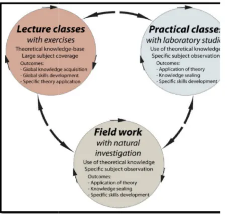
Generally modelling is a very wide term as used and applied in earth sciences. Regarding groundwater flow processes, the theoretical aspects taught in theory can effectively be illustrated in practical lab sessions, as well as in the field. Therefore, students can characterize phenomena at various scales in terms of time and space, and also with different approaches (comparison of several methods and formulas, empirical versus practical). An integrated pedagogical approach is defined by Gleeson et al. (2012), and then also by Hakoun et al. (2013), as the combination of three class components into one single teaching course. The loop presented in FIG 1 is the symbol of the cohesive and mutual relation between lectures, practical classes and field works. The continuity of that loop is the triggering point to stimulate the students’ interest and curiosity. The three components considered are:

1) Lectures and simple exercises, which have the purpose to set the course background and review all main basic notions, enhancing the students’ knowledge with new/advanced concepts, and introducing the technical field methodology;

2) Practical active lab experiments which aim to develop specific technical skills, introducing the learner to critical thinking, applying the theoretical concepts learned and using the problem-solving logistics related to the unpredictability of each experience (practice and theory are two different domains);

3) Field works in order to develop more specific abilities, re-calling all what was learned during the classes.

Hydrogeology benefits from the fact that many important processes can be illustrated and explained with simple physical models. And in fact the use of physical models to perform real-world activities is becoming a central point especially for civil and environmental engineers because it enhances the hands-on learning of groundwater topics (like basic

(25)

groundwater definitions, groundwater flow well hydraulics, contaminant transport As a consequence of the possible earth sciences) who may attend demonstrate the groundwater

conducted amongst academic hydrogeologists indicates that the greater part of the crucial topics in a hydrogeology course

hydraulic conductivity determination, Darcy’s law, gradient of h (Gleeson et al., 2012).

FIG 1 Integrated hydrogeology pedagogy associated to an iterative loop over three class components. Within loop, each component support

Computer simulation depends

made in selecting or deriving appropriate parameters for equations. model seeing nature at work is believing. However

approximation of the reality

behaviours that could lately be extended to many other situations Finally, physical models like groundwater tank

demonstrator but also as an instrument around which projects arranged (Parkinson, 1987).

24

groundwater definitions, groundwater flow together with the explanation of the well hydraulics, contaminant transport, and risk analysis).

possible broader range of students’ background ( who may attend a standard hydrogeology course, it is necessary to

groundwater basic concepts early in the teaching.

conducted amongst academic hydrogeologists indicates that the greater part of the crucial pics in a hydrogeology course are associated to groundwater flow processes

hydraulic conductivity determination, Darcy’s law, gradient of heads, and transmissivity

ntegrated hydrogeology pedagogy associated to an iterative loop over three class components. Within

loop, each component supports the others with chains of mutual feedback. Inspired from Gleeson et al. (2012) and Hakoun et al. (2013).

ter simulation depends after all on the programmer and on a list made in selecting or deriving appropriate parameters for equations. Whereas

model seeing nature at work is believing. However, the physical model is only an roximation of the reality, it could provide deep understanding of concepts and behaviours that could lately be extended to many other situations.

like groundwater tank, column of soil etc. are useful not only as lso as an instrument around which projects and dissertation work can be together with the explanation of the Darcy’s law, r range of students’ background (wide range of it is necessary to start to In fact, a survey conducted amongst academic hydrogeologists indicates that the greater part of the crucial to groundwater flow processes such as ads, and transmissivity

ntegrated hydrogeology pedagogy associated to an iterative loop over three class components. Within this iterative mutual feedback. Inspired from Gleeson et al. (2012)

list of assumptions Whereas with a physical the physical model is only an , it could provide deep understanding of concepts and , column of soil etc. are useful not only as sertation work can be

(26)

25

3. Dimensionality-based classification and examples of application

The numerous physical models are usually classified based on dimensionality: 0D, 1D, 2D, 3D. Lab experiences linked to them are going further and further increasing the model dimension, in the understanding of phenomena, gradually extending the validity of concepts and knowledge behind.

The easiest one that can be studied are the 0D batch models, where there is just a mix of water, sediments and chemicals. Through them are basically analysed only the reactions and not the flow. It can be investigated the different behaviour of several contaminant types: a dissolved contaminant (represented by liquid dye), a dense non-aqueous phase liquid (DNAPL) (represented by molasses), and a light non-aqueous phase liquid (LNAPL) (represented by olive oil). For example, a simple test aquifer model can be implement in a beaker (FIG 2): in this way it is possible to compare at least two different models, in terms of movement and remediation of the three aqueous contaminant types cited before, by applying simple pump-and-treat to each contaminant spill.

FIG 2 Aquifer model constructed by students for the groundwater remediation lab activity (Hilton, 2008)

1D models are then still very simple to be described, in terms of experimental set up and lab experiences implemented. They are basically and primary used to prove the Darcy's Law which is one of the most essential concepts in hydrogeology, thus a prerequisite before moving towards more complex issues. Demonstration were always given firstly through one-dimensional fluid flow models applied to saturated columns of porous media. The experimental apparatus is called permeameter, but other similar devices can be used, such as simple, inexpensive, high resistant plastic transparent columns. Those can have various dimensions (in length and diameter). Through them many relations and parameters can be studied: hydraulic gradient, porosity, fluid viscosity, particle size influence, volumetric flow rates, etc. (Werner et Roof, 1994; Nicholl et al., 2016).

In column experiments water is free to flow through the pores between soil particles in accordance with the Darcy’s empirical law (more theoretical notions behind are presented in the paragraph 4 and 5 of Chapter 1, concerning flow and transport equations).

(27)

26

The hydraulic conductivity (K) is a specific parameter used to quantify how well the water flows through a soil medium. It basically depends on the average size of the pores through the soil matrix, on how well the particles fit together, and on the temperature of the surrounding environment which is directly linked to the viscosity of the water (Akbulut, 2016). Those influences can be analysed through soil-column experiences, performing the same kind of test in different soil samples at different conditions.

Research and studies focused on 1D column experiments are the most ancient ones, and they are still widely used to compare and determine values of K and porosity (total, effective and of transport). Basically the flow is driven only by the hydraulic gradient, therefore, orientation of the sample in terms of gravity and references have no effect on the flow rate. Of course where the flow must pass across several different layers of materials, the one with the larger K is dominating the system (Nicholl et al., 2016). Once the Darcy’s law is proved, it is possible to move towards more complex problems related for example to transport phenomena. Also tracer test, both with ideal conservative tracer and with contaminants, can be implemented in order to obtain flow and transport parameters estimation (such as the dispersivity coefficient).

For K values estimation two main types of tests can be developed: the Constant Head Permeability Test in FIG 4, mainly for medium-coarse soils (Domenico et Schwartz, 1990; Ritzema, 2006; Cai et al., 2015; Hussain et Nabi, 2016; Nicholl et al., 2016); and the Falling Head one in FIG 3, which is more specific for finer type of medium (Stibinger, 2014; Johnson et al., 2005).

Other laboratory tests on soil-columns have been performed also to study the dispersion properties of uniform porous media, both in steady and transient flow conditions. The majority of experiences were tested in uniform matrix like glass beads (Rumer, 1962; Harleman, 1963; Lepage, 2013), sands (Blackwell, 1962; Harleman, 1963; Wierenga et Van Genuchten, 1989; Khan et Jury, 1990; Costa et Prunty, 2006; Kasteel et al., 2009; Mastrocicco et al., 2011; Steyl et Marais, 2014; Cai et al., 2015; Kanzari et al., 2015) and gravels (Rumer, 1962). Also analysis on non-uniform soils are available (Raimondi et al., 1959; Legatsky et Katz, 1966; Ujfaludi, 2010; Steyl et Marais, 2014 ; Mastrocicco et al., 2011).

The majority of all those studies are developed in saturated soil columns, but there are also researches on unsaturated samples (Childs et Collis-George, 1950; Vachaud, 1968; Philip, 1969; Swartzendruber, 1969; Parlange, 1971; Sakellariou-Makrantonaki, 2016). At the same time only a few attempts have been made to study the effect of non-uniform soil structures on the dispersion characteristics (Raimondi et al., 1959; Legatsky et Katz, 1966) even though natural soils, in most cases, consist of non-uniform particles (Ujfaludi, 2010). More details about procedures, equipment, and theory behind those applications will be presented in Chapter 3 while describing the work performed on four different types of sand.

(28)

FIG 3 Apparatus for hydraulic conductivi

FIG 4 Experimental setup of C

Concerning representations of physical a differentiated by an increase of complexity To study and understand some

of experiments can be performed content in the unsaturated zone, storage coefficient and the sa

recharge and discharge areas for groundwater, (through the use of an hand shower device),

system, pumping test (with the simple use of a syringe or a peristaltic pump), 27

Apparatus for hydraulic conductivity determination: Falling head test (Nicholl et al., 2016)

Constant-head test (black) and Tracer test (black and blue) (Cai et al.

of physical aquifer, there are both 2D and 3D of complexity (substantial increment in the thickness)

To study and understand some of those basics cited concepts among aquifers, a broad range of experiments can be performed primary in physical 2D models: influence on

ted zone, quantitative determination of hydraulic properties storage coefficient and the saturated hydraulic conductivity, runoff process,

ischarge areas for groundwater, drought period simulation, rain infiltration through the use of an hand shower device), piezometric head variations

system, pumping test (with the simple use of a syringe or a peristaltic pump), (Nicholl et al., 2016)

) (Cai et al., 2015)

and 3D physical models, (substantial increment in the thickness).

concepts among aquifers, a broad range influence on the water nation of hydraulic properties as the cess, significance of rought period simulation, rain infiltration variations, saturation of the system, pumping test (with the simple use of a syringe or a peristaltic pump), and injection

(29)

28

of tracer for transport parameter estimation (conservative tracer and probe recordings) (Hilton, 2008).

Typical dimensions of those considered 2D models are going from 40 cm up to 2 meters in length, from 20 cm up to 1 meter in height, and around few centimetres of thickness. As a consequence, the thickness is generally negligible compared to length and height and parameter associated to phenomena and behaviours in this direction are not investigated. As usual, in physical 2D model different soil layers are included: some are made by fine sand and some are coarse generally sand or gravel. In other cases, also karst, clay and silt can be present. The majority of those 2D physical models have two aquifers (as it can be seen in the schematic representations in FIG 5): an unconfined one, and a confined artesian one along the bottom. In fact, by inter-layering materials with different hydraulic properties multi layer aquifers can be created, confined and unconfined or artesian, porous or fractured (Farrell, 1997).

Many example of concepts and related demonstration experiences are reported in documents as “ Curriculum Guide to the Sand Tank Groundwater Model “ provided by Lane (n.d.), in “Groundwater flow demonstration model” written by Farrell (1997), in “ Physical models for classroom teaching in hydrology “ by Rodhe (2012). Furthermore Parkinson (1987) described an experimental sand tank developed for demonstrating the groundwater flow to drains under simulated rainfall.

Many variation of those open-sand plexiglass containers really exist (pictures inserted in Annex 0): they allow to study the influence of different geological structure or human build structure, etc.

The flow system for the kind of physical sand tank described is basically driven by two constant head reservoirs, one at each end side of the sandbox. Those types of systems are generally capable of maintaining constant head boundaries simultaneously by pounding water at the top in addition to fixing the hydraulic heads in the two constant head reservoirs (Illman et al., 2010).

Groundwater solute transport studies can also be carried on, with advection and dispersion being the first two mechanisms to be analysed, once groundwater flow is characterized. Then contaminant plume movement can be investigated through multiple sampling or directly visualized (Hilton, 2008).

(30)

29

FIG 5 Physical 2D model of an aquifer: scheme + real example (sources : Lane, Guide to Sand tank, and https://etc.usf.edu/clippix/picture/front-view-of-the-groundwater-model.html, consulted in July 2019)

3D sandboxes can also be used to observe various fluid flows and thus to validate some solute transport algorithms. Again several different experiences can be simulated, such as a simple steady state stable flow, transient flow, solute transport, pumping tests, flux measurements, etc. Early studies utilize uniform packing of sands to create a homogeneous medium and uniformly heterogeneous packing (Silliman et Simpson, 1987; Schincariol et Schwartz, 1990; Illangasekare et al., 1995, Illman et al., 2010).

(31)

More recently, also complex heterogeneity patterns have been packed by various researchers (Welty et Elsner,

Danquigny et al., 2004; Fernàndez

simulation of the variability of hydrau understanding and predicting solute transport

Many different implementations are possible: uniform sand,

media containing intermixed regions of coarse and fine sands. Different source zone release conditions can be arranged by modifying the

field, while the surrounding hydraulic conductivity field remained unchanged. Then the injection of tracer into the source zone should be followed by measuring concentrations as function of time at the location where tracer was

farther downstream (FIG 6). The resulting breakthrough curves can be characterized in terms of transport parameters (equation

Many experiments to investigate saltwater

were also studies on 3D box filled by sand or glass beads ( Brakefield, 2008; Goswami et al.,

FIG

30

complex heterogeneity patterns have been packed by various 1997; Silliman et al., 1998; Chao et al., 2000; Barth et al.

2004; Fernàndez-Garcia et al., 2005). In heterogeneous sandbox aquifer, variability of hydraulic conductivity as a function of space, standing and predicting solute transport can be implemented.

Many different implementations are possible: uniform sand, layered sand, and two

media containing intermixed regions of coarse and fine sands. Different source zone release conditions can be arranged by modifying the hydraulic conductivity of the injection near field, while the surrounding hydraulic conductivity field remained unchanged. Then the injection of tracer into the source zone should be followed by measuring concentrations as function of time at the location where tracer was injected and in a detection zone located

The resulting breakthrough curves can be characterized in terms equations in paragraph 5) (Gueting et Englert, 2011).

Many experiments to investigate saltwater intrusion and mixing of different densit were also studies on 3D box filled by sand or glass beads (Luckner et Schestakow,

et al., 2011).

FIG 6 Experimental sandbox set up (Jose et al. 2004)

complex heterogeneity patterns have been packed by various 2000; Barth et al., 2001; In heterogeneous sandbox aquifer, as a function of space, for layered sand, and two or plus media containing intermixed regions of coarse and fine sands. Different source zone release vity of the injection near field, while the surrounding hydraulic conductivity field remained unchanged. Then the injection of tracer into the source zone should be followed by measuring concentrations as a detection zone located The resulting breakthrough curves can be characterized in terms

2011).

intrusion and mixing of different densities fluid et Schestakow, 1991;

(32)

31

3D sand tanks are also exploited to measure groundwater fluxes in a well bore of reference (FIG 7). Based on theoretical predictions and experimental evidence, researchers have been using 3D physical models to validate many groundwater flow velocity and fluxes measurement techniques such as:

1) For FLUX (passive techniques)

i. Passive flux meters PFM (Kearl, 1997; Graw et al., 2000; Hatfield et al., 2004; De Jonge et Rothenberg, 2005; Basu et al., 2006; Borke, 2007; Wu et al., 2008) ii. iFLUX cartridges (Verreydt et al., 2017)

2) For FLOW RATE and then FLUX (dividing the flow measured by the superficial surface of flow)

i. Borehole dilution methods (Drost et al., 1968; Grisak, 1977; Giercsak et al., 2006 ; Pitrak et al., 2007)

ii. Point dilution method PDM and Finite volume FVPDM (Batlle-aguilar et al., 2007; Piccinini et al., 2016; Jamin et Brouyère, 2016-2018)

iii. Direct velocity tool DVT (Essouayed, 2019) 3) For FLOW VELOCITY

i. Colloidal borescope CB (Kearl, 1997)

ii. Point velocity probe PVP (Labaky et al., 2007; Devlin et al. 2010-2012) and In-well PVP (Devlin et al., 2018)

iii. Acoustic doppler velocimeter ADV (Kraus et al.,1994; Wilson et al., 2001) iv. Laser doppler velocimeter LDV (Momii et al., 1993)

v. Heat-pulse flow meter (Hess, 1986; Kerfoot, 1988)

The added value of lab-scale physical models compared to field-scale experiments is the feasibility: physical models in fact need less time to completely show results of an experience. Thus they allow easier and faster demonstration of concepts and allow direct observations of phenomena. Through them an immediate understanding of water-soil behaviour and interactions is possible. A preliminary approach to get closer to problem-solving and practical issues, starts also to be developed through those experiences in lab. On the other hand, field experiments are closer to reality and allow to develop strategy to deal with practical projects (real site dimension and heterogeneity, real equipment and set up of investigations, etc...).

(33)

32

FIG 7 Lab-scale flow tank: A-Colloidal borescope (Wu et al. 2008) and B-Monitoring well (Verreydt et al. 2015)

A

(34)

33

4. Description of flow equations and associated parameters

While building a numerical model as a reference of a physical system, there are some characteristics to assure. Firstly the model has to be both physically and numerically consistent, meaning that it has to be based on conceptual choices able to simplify the reality in an efficient way and the errors tend to zero for decreasing mesh increments and time steps. It has to be accurate (lower modelling errors), and with quite high resolution. Groundwater flow equations behinds models, are then generally associated to representative elementary volume (REV), which is a finite volume of geological medium used to quantify different properties associated to it. To define a REV, generally the medium should be both continuous and porous, because equations are developed in a continuous dimension. In MODFLOW, the software used in this work, this REV is generally associated to each cell of the model implemented. Additionally, the presented case is related to lab tests, so the used scale is a macro scale, generally ranging between centimetres to few meters, and able to be representative for medium properties. A list of the most relevant ones and their description is reported. All mentioned variables and parameters are defined here, therefore once they will be mentioned afterwards in the documents no further explanations will be given.

4.1 Bulk and particle densities

The bulk density (ρbulk) is defined as the dry soil weight divided by the volume of solid soil

together with the pores. For mineral soils it commonly ranges from 1.1 to 1.5 g/cm3_{, and it}

increases with depth. It tends also to be high in sands and low in soils containing a relevant amount of organic matter. Furthermore, it is conditioned by the process of compaction: higher degree of it tends to raise the value of ρbulk. It is also known that the high bulk

densities generally correspond to low porosity.

The bulk density differs from the so called particle density (ρ), which is the volumetric mass of the solid soil that does not take in account the pore spaces and represents the average density of all the minerals composing the soil. For most soils, this value is around 2.65 g/cm3, mainly because quartz has a density of 2.65 g/cm3 and it is usually the dominant mineral. Particle density varies little between minerals and generally it does not have a big practical significance, except in the calculation of pore space.

4.2 Porosity: total and effective

Total porosity (ntot) is the portion of the soil volume occupied by pore spaces. It is generally

quantified as a percentage. This property does not have to be measured directly since it can be calculated using values determined for bulk density and particle density with the formula:

(35)

34

Total porosity can be classified as primary or secondary. The primary one is associated to the deposition of the sediments and includes interconnected pores together with the isolated ones, whereas secondary porosity is formed after and includes cavities produced by several phenomena as the dissolution of carbonates, fracturing, etc. Secondary porosity is not considered in the presented case (especially during column experiments described in Chapter 3) because of the homogeneity of the soil used for each sample (sorted sand) and the configuration of the system (as a 1D column experiments).

Effective flow/drainage porosity (neff,flow) is the portion of the total void space of a porous

material in which is really passing the fluid. Effective flow porosity exists mainly to explain the fact that a fluid in a saturated porous media will not flow through all voids, but only through the interconnected ones. It is expressed as a percentage and it is basically calculated as:

neff,flow (%) = × 100

The un-connected spaces are known as dead-end pores and their presence and quantity depend on particle size, shape, and packing arrangement. There is also a portion of fluid contained in interconnected pores which is held in place by molecular and surface-tension forces. This portion is generally known as "immobile" fluid volume and it is not part of the real fluid flow. In many practical cases such as the calculation of travel time of difference substances through porous materials, requires knowledge of this effective flow porosity (Stephens et al., 1998). Effective or either kinematic flow porosity usually cannot be measured in absolute terms so normally it refers to the volume of fluid released by drainage of a saturated medium after a finite interval of time. The formula to analyse is:

neff,flow (%) = × 100

where small v is the mean velocity of the fluid (m/s) and q is the specific discharge or Darcy’s flux (m/s), calculated as q = Q/A in which Q is the flow rate (m3/s) and A, the area section (m2).

Total porosity generally increases with decreasing grain size, and the portion of interconnected pore space with respect to the total pore space, following the definition :

ntot (/) = Sy + Sr = neff,flow + Sr

where the specific yield Sy (which is < ntot) which is either dimensionless either a percentage,

and represents the volume of water released from storage by an unconfined aquifer per unit surface area of aquifer per unit decline of the water table (Bear, 1979). This equals the effective flow porosity in case of unconfined aquifer (Sy = neff,flow). Then, Sr is the specific

retention or either retention capacity (dimensionless or a percentage), calculated as the ratio between the volume of immobile water divided by the total volume of the sample.

(IV) (II)

(36)

35

Normally another parameter can be defined: the effective transport porosity (neff,transport),

which is lower than the effective flow porosity, which is lower than the total porosity. This parameter is expressed as a percentage and it is calculated as:

neff,transport (%) = × 100

where the volume of mobile solute is generally lower than the volume of mobile water.

4.3 Hydraulic head

The hydraulic head (h), also called water head or either piezometric head, under the hypothesis of an homogeneous incompressible fluid, describes the potential energy of the system at any point. It is calculated as :

h = z + ( _× ) [in m]

where z is the elevation (m) above the reference chosen, g is the value of the acceleration of gravity (equals to 9.81 m/s2_{), P is the pressure (Pa = N/m}2_{= kg x m/s}2_{) and ρ}

fluid is the density

of the fluid (taken as 1000 Kg/m3 _{in case of water). Practically speaking, the hydraulic head}

can be defined as the height above the reference level to which the fluid will rise in a manometer, and it is given by the sum of the altitude or elevation plus the pressure head.

4.4 Darcy’s Law, Hydraulic conductivity and effective velocity

The Darcy’s Law, which firstly describes 1D laminar flow through any kind of saturated porous medium (such as rocks, soil, ...) is one of the most essential concept in the study of hydrogeology. Henry Darcy in 1856 performed his original experiments in the context of municipal water filtration for the city of Dijon, France. Unable to find an existing relation between flow rate and filter size, he performed a series of experiments to have several data available for calculations. Briefly the experiences consisted in pressurized water entering the top of a sealed vertical column filled with sand and exited through a tap at the bottom. Using manometers, Darcy measured the hydraulic heads (h) at the inlet and outlet section of the column. Through those experiments, for a chosen type of sand, he observed that the flow rate (Q) is proportional to the cross-sectional area of the column (A), to the difference between measured water levels inlet and outlet (Δh), and to the inverse of column height (1/Lcolumn). He discovered that the coefficient of proportionality is varying depending on the

type of sand used. In particular he pointed out that generally a coarser sand have a larger coefficient of proportionality than a finer one. This Darcy’s coefficient of proportionality is the so called hydraulic conductivity (K).

(V)

(37)

36

Hydraulic conductivity (K) is one of the principal and most important soil hydrological parameter. It is a relevant factor for the evaluation of the water flow, infiltration processes and transport within a medium. Hydraulic conductivity is generally expressed by units of velocity (m/s or cm/s or m/h, etc.).

Fluids tend to flow towards the decreasing hydraulic head, therefore the need to put a negative sign in Darcy’s equation (in order to make volumetric flow rate Q a positive quantity) while describing the hydraulic conductivity:

𝐾 = ×_× =

× [in m/s] (VII)

Where i is the hydraulic gradient (obtained as Δh/Lcolumn), and Lcolumn is the column length

(m).

Subsequent to Darcy’s original experiments, in case of porous media it was discovered that measures of K increase with ρfluid and are inversely proportional to fluid dynamic viscosity (µ

in Pa·s or N·s/m2 or kg/m·s). So in 1940 the scientist Hubbert suggested the existence of an innate material property called intrinsic permeability (k) that is linked to the hydraulic conductivity through the ρfluid, µ and g:

k = × _× [in m2] (VIII) Darcy’s flux (q) in 1D system (such as columns) can be expressed as:

𝑞 = 𝐾 × 𝑖 = 𝐾 × [in ]

Where x is the distance taken in the direction of the groundwater flow. Equation IX assumes that flow occurs through the entire cross section of the material without regard to solids and pores. However, Darcy flux is not the actual fluid velocity in the porous media, but it is just discharge rate (Q) per unit cross-sectional area.

A scheme of the Darcy’s Law is reported in the FIG 8. 1.

FIG 8 Darcy’s Law (source: PPT Permeability in soils, Geotechnical Lab, Civil Eng Texas University) (IX)

(38)

37

The extension to 3D case is associated to eq. (XII) where the 3D Darcy’s flux 𝑞 (m/s) equals: 𝑞 = − 𝐾 × 𝑔𝑟𝑎𝑑(ℎ) = − 𝑘 × × [ 𝑔𝑟𝑎𝑑

× + 𝑔𝑟𝑎𝑑(𝑧) ]

and 𝐾 is the so called hydraulic conductivity tensor (as well as 𝑘 is the permeability tensor) associated to the directional components of the parameter, therefore used to express anisotropy (heterogeneity) or isotropy of the investigated porous medium. Moreover, the 3D gradient of hydraulic head 𝑔𝑟𝑎𝑑(ℎ) is composed by ( ; ; ).

The actual seepage velocity of groundwater, also named effective velocity of flow veff,flow

(m/s) depends on the real portion of mobile fluid and on the available cross-sectional area through which the flow is occurring. Its value is estimated as:

veff,flow =

, ×

∆

=

, in [m/s]

Usually the K-values are strictly dependent both on fluid properties and on material(s) properties. Moreover, in case of soil layers, vertical degree of permeability is very often different from the horizontal one because of the presence of vertical differences in terms of structure, texture, porosity of the soils. Only in some structure-less soils, as the case of sands, the K is considered to be the same in all directions.

Another important observation is that Darcy’s law is not valid when the flow is not laminar, for example when Re > 1. Reynolds number Re is a dimensionless quantity used in fluid mechanics to help to predict flow patterns in different fluid flow situations. It is :

𝑅𝑒 = 𝜌 𝑣 𝐿′

𝜇 =

𝑣 𝐿′ ʋ

Where L’ is the characteristic linear dimension (m) and ʋ is the kinematic viscosity of

the fluid (m2_/s).

4.5 Groundwater flow in steady state conditions

Under steady state conditions, meaning where no variations of the system over the time are considered, the groundwater flow equation is a composition of the Darcy’s law and the conservation of water (in terms of mass or volume, equals in- and out- flows). Those conditions represent the equilibrium and stabilization of a system, thus there are no changes in storage. While implementing steady state conditions, initial conditions will not really affect the final results. However, a good initial condition will lead to a fast and stable convergence of the numerical solver.

There is no time dimension because there are no variations in time, so results are easier to be visualized. And certainly errors in the model set up could be more evident in the final results.

(XII)

(XI) (X)