ALMA MATER STUDIORUM
UNIVERSITÀ DI BOLOGNA
SCUOLA DI SCIENZE - CAMPUS DI RAVENNA
CORSO DI LAUREA MAGISTRALE IN BIOLOGIA MARINA
Exploring the distribution and underlying drivers
of native and non-native mussel and oyster
species in harbour environment
Tesi di laurea in: “Ecosistemi Marini: Struttura e Processi”
Relatore Presentata da
Prof.ssa Laura Airoldi Francesco Mugnai
Correlatore
PhD Francesco Paolo Mancuso PhD Federica Costantini
II sessione
Abstract
The increase of human population and their pressures in coastal areas is causing an exponential sprawl of artificial structures in marine areas, leading to the loss of natural habitats. Artificial structures are characterised by low species richness and a prevalence of non-native species compared to natural rocky reefs. Commercial and tourist ports are examples of artificial habitats. Little is known about the distribution and dynamic of the species inhabiting ports, and the factors leading to a prevalence of non-native species in these habitats are still not fully understood. Here, the distribution and abundances of two native (Mytilus galloprovincialis, Ostrea edulis) and two non-native (Xenostrobus securis,
Crassostrea gigas) bivalve species that grow on the artificial seawalls of the 11 km long canal
port of Ravenna were assessed to: 1) explore their distribution in different areas of the harbour, and 2) identify whether the observed patterns were related to variations in environmental variables (seawater pH, salinity, temperature, dissolved O2 and nutrients) or
to variable supply of larvae reaching different areas of the port and settling on the artificial seawalls. DNA extraction and amplification protocols were developed to barcode the bivalves settlers due to the impossibility to identify them microscopically. Results showed an increase of non-native species as the canal-port goes inland. Temperature, oxygen and nitrate seawater concentration explained most of the variation in species abundance among sites. The non-native mussel X. securis was associated to higher sea surface temperatures compared to the native M. galloprovincialis. Settler abundances were clearly correlated to the spawning window of the species, but not to the abundance of adults on the seawalls, suggesting a prevailing role of post-settlement processes. Future work should explore the potential role of other environmental variables (water circulation, drainage), extend the duration of the observations, and use a metagenomics approach to characterise propagule pressure dynamics in the water column.
SUMMARY
1. INTRODUCTION ... 5 1.1. The harbour environment ... 7 1.2. Non-native species on artificial structures ... 9 1.3. Previous research ... 11 1.4. Aims of the thesis ... 14 2. MATERIALS AND METHODS ... 16 2.1. Study site ... 16 2.2. Experiment design ... 17 2.3. Environmental parameters ... 18 2.4. Distribution of native and non-native mussel and oyster species ... 19 2.5. Spatial-temporal variability of settlers ... 20 2.6. Genetic analysis ... 21 2.6.1. DNA extraction ... 22 2.6.2. PCR amplification protocol ... 22 2.6.3. Agarose gel run ... 23 2.6.4. Sanger sequencing plate preparation ... 23 2.7. Statistical analysis ... 24 2.7.1. Distribution of sites by environmental parameters ... 24 2.7.2. Spatial distribution of native and non-native mussel and oyster species ... 24 2.7.3. Relationship between seawall adults and environmental variables ... 25 2.7.4. Settlers spatial-temporal variability analysis ... 25 2.7.5. Relationship between seawall adults and settlers abundances ... 25 3. RESULTS ... 26 3.1. Environmental variables ... 26 3.2. Changes in abundances of seawall mussels and oysters ... 27 3.2.1 Adults samples analysis ... 27 3.2.2. Mussel species distribution ... 28 3.2.3. Oysters species distributions ... 30 3.2.4. Relationship between environmental variables and adults ... 32 3.2.5. Settlers spatial-temporal variability ... 343.2.6. Correlation between settlers and adult abundance ... 35 3.3. DNA extraction and amplification from a single settler ... 36 4. DISCUSSION ... 38 5. CONCLUSIONS ... 41 6. REFERENCES ... 42 7. SUPPLEMENTARY MATERIALS ... 50 8. AKNOWLEDGEMENTS ... 53
1. INTRODUCTION
The coastal zone forms a narrow interface between marine and terrestrial areas, extending inland 70 – 100 km and offshore to the edge of the continental shelf (Crossland et al., 2005). Although this zone comprises less than 20 % of the Earth’s surface, it houses more than 45 % of the human population. In addition, 17 megacities of the world (cities or urban agglomerations with more than 10 million inhabitants) are located along the coasts and have a strong influence on coastal marine habitats (Crossland et al., 2005; Von Glasow et al., 2013).
Humans depend on coastal environments for food, energy, construction, transport, recreation and many other resources and services. Over the last century, the exponential growth of human population in coastal areas and the related intensification of activities such as fishery, ship trading, oil and gas extraction and summer tourism has led to a loss of coastal habitats (Airoldi et al., 2009). As a consequence, we assisted to an exponential increase of various artificial structures sustaining human activities (Table 1). Table 1: Examples of coastal human activities and related artificial structure. HUMAN ACTIVITY RELATED ARTIFICIAL STRUCTURES Coastal protection and structural management seawalls, breakwaters, revetments, dykes, groynes, jetties, pilings, bridges, artificial reefs Energy production wind turbine, floating and fixed offshore wind turbine and wave energy converter Mining oil and gas platforms Aquaculture cages Recreational, cultural and scientific activities artificial reefs, wrecks
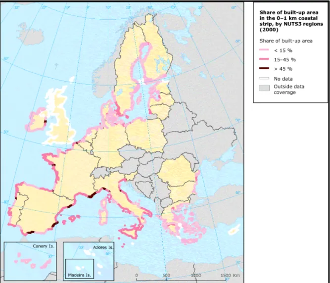
Nowadays, more than the 50 % of the natural coastal environments are transformed by some hard engineering around the most developed countries (Europe, Asia, USA, Australia). In Europe around 22,000 km2 of coasts are armoured, and concrete dominates beyond 50% of Italy, Spain and France shorelines (Figure 1) (European Environment Agency, 2006). The increase of coastal development has led to the loss of essential habitats rich in species and genetic diversity such as saltmarshes, seagrass meadows, rocky shores, coral reefs, mangrove forests, mudflats and oyster reefs (Airoldi et al., 2008; Airoldi et al., 2009; Munday, 2004; Walker & Kendrick, 1998).
Figure 1: Coastal built-up zones in 0-1 km from coastal shore (based on Corine land cover, 2000. 24 (E. E. A., 2006).
Together with the loss of these ecosystems, another major ecological concern is the growing evidence that artificial structures do not function as natural rocky or biogenic habitats. Indeed, numerous studies document distinct species assemblages inhabiting such structures (Bulleri and Airoldi, 2005; Bulleri and Chapman, 2004; Glasby et al., 2007; Moschella et al., 2005), local loss of particular functional groups - such as large grazers and predators - (e.g., Bulleri and Chapman, 2004), low species and genetic diversity (Bulleri and Chapman, 2004; Fauvelot et al., 2009; Johannesson and Warmoes, 1990), the presence of floral and faunal communities that are often at an early stage of succession (Bacchiocchi and Airoldi, 2003; Bulleri and Airoldi, 2005; Glasby et al., 2007), and different ecological interactions (Iveša et al., 2010; Klein et al., 2011) and functions (Bulleri et al., 2005; Martins et al., 2009; Moreira et al., 2006; Perkol-Finkel and Benayahu, 2009). Moreover, the ecological effects of artificial
native species and acting as ecological corridors for their dispersal (Dafforn et al., 2012). The reasons facilitating non-native species in artificial habitats are not fully understood yet. Potential explanations include a variety of factors, such as: the high disturbances in artificial habitats that often maintain large amounts of bare spaces (Airoldi & Bulleri, 2011), the fact that artificial substrates usually are located near anthropogenic sources of organic matter and pollutants, which are known to favour non-native species (Piola & Johnston, 2008), or their location near some of the most important entry pathways represented by ports, where the propagule pressure of non-native organisms transported by maritime activities is notoriously very high (Nall et al., 2015).
1.1. The harbour environment
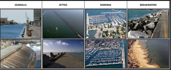
Commercial and tourist harbours are examples of environments where we can find lots of artificial structures (Figure 2). These structures, built at the interface between the land and sea, facilitate activities such as transport (shipping of cargo, passenger ferries and cruise liners), industry (development of commercial properties and extraction/utilization of resources), residential development, commercial and recreational fishing, recreational activities (boating and beach going) and cultural activities (e.g. festivals). Harbour waters and sediments often become enriched with nutrients and pollutants such as heavy metals, metalloids, and organic contaminants mainly from industries, losses of fuels from ships and boats and discharge of sewage pipe systems. As a consequence, physic-chemical variables such as sea surface temperature, salinity, dissolved oxygen (DO), pH, conductivity, turbidity and nutrient concentration can result profoundly altered in harbour environment (Dafforn et al., 2009). Changes in these variables may affect the growth and reproduction rates of resident species and alter their metabolic support and feeding efficiencies (Ostroumov, 2005; Salazar and Salazar, 1996).
Figure 2: Examples of artificial structures in harbour environment.
Marine harbour infrastructures are characterised by flat surfaces, both vertical and horizontal, that lack of essential microhabitats that can protect organisms from environmental stressors. This aspect can influence both the distribution and abundance of species colonising the artificial hard substrate. Usually, seawalls, one of the more common forms of harbour armouring, support lower diversity with homogenous species composition, mostly dominated by opportunistic and/or non-native species (Chapman, 2003; Richmond and Seed, 2009). Since seawalls are constructed using human-made materials (such as concrete), their chemistry may differ from natural rocky reefs (e.g. concrete pH content) affecting the type and number of species that can grow on it (Perkol-Finkel and Sella, 2014). Indirect consequences of the presence of harbour infrastructures can be the modification of environmental variables such as light exposure, sediment load, currents, temperature and other abiotic factors, which can evolve into more homogenous conditions compared to those at natural rocky reefs (Airoldi, 2003; Irving and Connell, 2002). Moreover, the species composition and dynamic of the benthic assemblage in harbour environments can be affected by propagules of non-native organisms transported in the ballast water of ships (Nall et al., 2015).
Nowadays, there is growing attention towards eco-engineer solutions to rehabilitate vital communities onto artificial marine structures. Building “greener” structures for example by incorporating greater morphological complexity, can enhance the settlement and recruitment of local native organisms. In those structures that mimic the natural reefs and
al., 2007). However, identify the best alternative solutions to build artificial structures in harbour environment requires an in-depth knowledge of the distribution and dynamic of the species present inhabiting them.
1.2. Non-native species on artificial structures
During the last century, the development of modern human societies and the globalisation caused the transport of species and their establishment in places where they would have been unlikely to occur without human intervention. Species transported across major geographical barriers by human activities are known variously as alien, non-indigenous, non-native, exotic or introduced (Mineur et al., 2012). Usually, the term invasive (whether referring to species, stages, or populations) relates to cases that involve adverse ecological or economic impacts. Here, we use the term non-native species to indicate species, at any stage in the establishment, outside their natural range due to both intentional or unintentional human effects (European Environment Agency, 2006).
As anticipated before, artificial structures (especially in harbours and ports) facilitate non-native species (Bulleri and Airoldi, 2005). These species can have a higher capacity of adaptation to adverse environmental conditions and a higher propagule pressure compared to native species (Clark and Johnston, 2009). Populations of native species, contrarily, tend to have much lower colonisation rates in artificial compared to natural habitats (Airoldi et al., 2015).
Significant pathways for the spread of alien species across biogeographical regions include shipping (ballast water and hull fouling) and aquaculture, including stock transfer and unintentional introductions via escapes and hitch-hikers and canals (Mineur et al., 2012). The risk of transportation and introduction of non-native species is very high in harbour environments, and ports and marinas are recognised as significant invasion hotspots (Carlton, 1987). Hulls of boats, ballast tanks and sea chests are all known vectors of non-indigenous species at both the larval or adult/mature stages. The invasion process is facilitated for those species that have a broad environmental tolerance because they can survive the process of entrainment and transport (Clark and Johnston, 2009). As previously mentioned, non-native species introduced into a new habitat can exploit environmental conditions that usually are not suitable for the growth of native species (Paavola et al.,
2005). For example, in Japan, Makabe et al. (2014) have reported an amplification of the jellyfish Aurelia aurita blooms following the installation of a floating pier in a fishing port. In the Mediterranean Sea during the 60s, the introduction of the non-native Pacific oyster
Crassostrea gigas led to a collapse of the native flat oyster Ostrea edulis with negative
economic repercussion (Molnar et al., 2008). The non-native mussel species Xenostrobus
securis is threatening native mussels along Spanish, French and Italian coastlines (Barbieri et
al., 2011; Garci et al., 2007; Gestoso et al., 2016; Giusti et al., 2008; Lazzari and Rinaldi, 1994). This species was introduced via aquaculture activities.
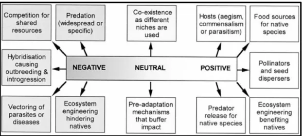
According to Goodenough (2010) (Figure 3), non-native species can have both positive and negative impacts towards native ones. Positive impacts are intended to represent a long-term fitness advantage, leading to an expansion of the native population. Non-native species can create positive interactions with native species (i) acting as a host, (ii) giving food support, (iii) altering the native ecosystem positively, or (iv) reducing the predation pressure. Negative impact of non-native species on native biota are intended to represent a reduction in fitness and abundance, eventually leading to a population decline. Non-native species can (i) be predators, (ii) be competitors, (iii) hybridise with native species, (iv) transport pests and diseases and (v) alter the native ecosystem. Besides, non-natives can also produce neutral effects through (i) an equilibrium phase between native and invasive species and (ii) an adaptation of the invasive species to the new environment.
Figure 3: Graph resuming the range of impacts that non-native species can have on native species (Goodenough, 2010).
and/or disease of native species can lead to reductions of the number of individuals and ultimately drive population decline or local extinction). Indirect ecological effects can be related to habitat destruction and interspecific competition; while indirect genetic effects can lead to inbreeding depression, together with hybridisation and ingression of genes. The indirect effects usually can lead to genetic changes in native species (Silva et al., 2009) (Figure 4). Figure 4: Direct and indirect impacts of non-native species on native ones (Silva et al., 2009). Identifying the factors facilitating the establishment and the distribution of non-native species, as well as the ecological interaction with native species, is crucial to safeguard natural marine ecosystems.
1.3. Previous research
Several studies highlighted the critical role of large shipping ports as a major pathways to the introduction and spread of non-native mussels (Micklem et al., 2016; Clarke Murray et al., 2011). For example, harbours represented the source of introduction for the mussel Mytilusgalloprovincialis in various localities around the world (South Africa, Hong Kong, Japan,
Korea, southeast Australia, Hawaii, Mexico, California, Washington, and the west coast of
Canada) (Branch & Steffani, 2004). Similarly, the green mussel Perna viridis (a native Indo-Pacific species) is spreading towards Durban Harbour, South Africa. Invasion of this green mussel has also been reported along the coasts of the British Columbia (Canada), together with other species of molluscs, which used the recreational boating as a dispersal vector. Although the role of harbours in the introduction of non-native species is well-known, few studies have explored the distribution and the dynamic of interaction between native and non-native species in harbour environments and how their dynamic is correlated with environmental parameters. For example, Queiroga et al. (2017) used trace elements contained in the mussel Mytilus galloprovincialis to analyse the spatial and temporal variability of the species across a period of 6 months. They discovered a possible link between connectivity patterns of this mussel and the phenomenon of upwelling/downwelling episodes during each season. Simon et al. (2017) explored the genetic connectivity in species of Mytilus (M. edulis, M. galloprovincialis and M. trossulus) and showed partially isolated subsets of each phenotypic species with different levels of local single nucleotide polymorphisms (SNPs) in the genotypes. Moreover, the reproductive isolation between the different species determined the genetic population structure, as the different Mytilus species “hybridise each time they meet” (iMarCo 2017).
Mussels and oysters exhibit a similar life cycle with an external spawning followed by a variable period (days-weeks) of free-swimming larval stages (trochophora, veliger,
pediveliger larvae). When the larva reaches the substrate (organic or inorganic), the
settlement process begins and the larva metamorphoses into a settler (generally < 400 µm in size) while over 400 µm the settler becames a recruit (Bownes et al., 2008; Ludford et al., 2012). The life cycles of mussels and oysters are shown in Figure 5 A-B respectively.
Figure 5: Details of the life cycle of mussel (A) and oyster (B).
In South Africa, several studies explored the interaction between different life stages (larval, settler, recruit and adult) stages of native and non-native mussels (Ludford et al., 2012; Porri et al., 2006a, 2006b). Porri et al., (2006) found a strong temporal variation in abundances of larvae and settlers of Perna perna but no correlation between the two. Moreover, no spatial effect was detected for larval availability, while there was strong spatial variation in settlement at the location level. They concluded that the patchiness in settlement observed at scales of 100s m depends on differential delivery, spawning period of larvae rather than their distribution offshore, suggesting that differential delivery is due to the effect of nearshore bottom topography on local water circulation. These processes are difficult to study as the firsts stages of mussel’s species are difficult to identify. Bownes et al. (2008) developed an identification method to discriminate between native Perna perna and
Choromytilus meridionalis and non-native Mytilus galloprovincialis. This method is able to
distinguish organisms from 300 µm up to 5 mm in size using a dissecting microscope based on marking and shape of the shells. However, the identification of the first stages of mussels and oysters remains a challenge, because the shells of Mytilus species are similar and their shapes can vary depending on the environment. Furthermore, some Mytilus species (e.g. M.
galloprovincialis and M. trossulus) can hybridise (Suchanek et al., 1997). Then, genetic
analyses are necessary for unequivocal identification.
1.4. Aims of the thesis
Ravenna is one of the most important Italian harbours along the Adriatic Sea (Airoldi et al., 2016). This port is an Italian leader of ship trading towards the Eastern Mediterranean and the Black Seas, particular for cereal, flour and fertiliser solid bulks, and is an essential slipway for general cargos and containers. Currently, the Ravenna harbour is one of the model study harbours within the international network World Harbour Project (WHP). The network aims to link, facilitate and enhance programs of research and management across major urban harbours of the world (http://www.worldharbourproject.org). The University of Bologna, co-leads the Workgroup 2 (WG2) Green Engineering. The WG2 aims to explore the distribution and the effects of the artificial structures in global harbours and to investigate materials and designs for an ecological engineering of harbours. In this perspective, my thesis aims to fill in knowledge gaps concerning the abundance, distribution and type of species that live in this environment, with particular interest to the interactions between native and non-native species. This fundamental knowledge is critical to identify eco-engineer solutions minimising the ecological footprint of artificial structures in harbour environments. The thesis explores the distribution of native and non-native mussel and oyster species in harbour environment. I focused my attention on two native species Mytilus galloprovincialis (Lamarck 1819) and Ostrea edulis (Linnaeus 1758), and two non-native species Xenostrobus securis (Lamarck 1819) and Crassostrea gigas (Thunberg 1793). M. galloprovincialis is a species native to the Mediterranean Sea. In the North Adriatic sea,this species tends to spawn mostly during the winter due to the lowest sea surface temperatures, and adults can grow up to 8 cm (Ceccherelli and Rossi, 1984).
X. securis has been found in the north-western Adriatic Sea since 1994 (Garci et al., 2007;
Lazzari and Rinaldi, 1994) and originates from Australia and New Zealand. It has a high tolerance for variations in sea surface salinity and temperature (Wilson, 1969). This species has also a high physiological mechanism in response to osmotic shocks (Wilson, 1969). X.
securis spawns mostly during the summer (Wilson, 1969).
Concerning oysters species, O. edulis is a native species to the Mediterranean Sea where it spawns in July (Bataller et al., 2006). However, its presence was drastically reduced by the parasite Bonamia ostreae carried by the introduced C. gigas for aquaculture purposes (Iglesias et al., 2005). C. gigas is native to the Pacific coast of Asia, and has a spawning period from April to August (Massapina et al., 1999). Nowadays, the abundance of O. edulis has severely declined in the northern Adriatic Sea (Beck et al., 2011)
Mussels and oysters represent the dominant bivalve taxa on the seawalls bordering 11 km long canal-port of Ravenna, and their distribution seems to change across various sites of the canal-port (Abbiati and Ponti, unpublished data). Variation in their distribution and abundance could be driven by environmental gradients along the canal-port and/or by differences in propagule pressure (e.g. reproductive period and/or the number of larvae and recruits on artificial structures) between native and non-native species. The thesis aimed to identify what are the main drivers that affect the distribution of the 4 target native and non-native species (M. galloprovincialis, O. edulis, X. securis and C. gigas), I deployed an experiment at 5 sites in the intertidal zone along the seawalls of Ravenna canal-port. An orthogonal design was used to test the following hypotheses: 1. The distribution and abundances of the native and non-native species that grow on the artificial seawalls change among different sites along the outside-inside gradient of the canal-port
2. Any observed difference is related to either co-occurring changes in the main environmental variables (seawater pH, salinity, temperature, dissolved O2, nutrients), or to differences in the supply of settlers that reach and establish on the seawalls.
To discriminate taxonomically similar bivalve species at this early stage of their life-cycles, I developed a DNA extraction protocol to amplify a barcode region (Cytochrome oxidase subunit I) from single bivalve recruits.
2. MATERIALS AND METHODS
2.1. Study site
The study was performed in the canal-port of Ravenna (for general information about the harbour and its environmental challenges refer to Airoldi et al., 2016). Ravenna is the largest city of the Emilia-Romagna coast border (north-western Adriatic Sea) with around 159,000 inhabitants. The city hosts one of the largest commercial inland port of Italy (Figure 6) with a waterway canal extending for 11 km from the centre of Ravenna to the tourist seacoast. Figure 6: The Ravenna canal-port.The banks of the canal (named Candiano canal) host various activities, including refiner petroleum industries, carbon and steel industries, agronomical production activities and energy power stations. The canal port is connected to the north and the south with two surrounding lagoons, named Pialassa Baiona (Figure 1 A) and Pialassa Piomboni (Figure 1 B) respectively, which are comprised of the southern part of the Po Delta Park. The Pialassa Baiona lagoon has a structure of canals and ponds divided by artificial embankments that receive water inputs from five main channels that drain a watershed of 264 km2, including
urban (9 %) and agricultural (87 %) areas. Nutrient levels are unusually high in the southern areas of the lagoon that also collects wastewater coming from urban and industrial sewage
treatment plants and two thermal power plants (Ponti et al., 2005). The Pialassa Piomboni lagoon, instead, has no freshwater supplies.
In the last 50 years, human activities have deeply modified the coast introducing large amounts of novel artificial hard substrate (breakwaters, groynes, jetties, pilings and offshore platforms) providing both subtidal and intertidal surfaces for the colonisation of introduced benthic organisms (Airoldi et al., 2016; Ponti and Airoldi, 2009). The development of the harbour has also affected the surrounding coastal areas, with the construction of two large converging jetties (≈ 2,400 m long each) to protect the harbour doorway from siltation altering the sediment transport and shaping the nearby highly-tourist beaches. Inside the port, seawalls constitute the predominant artificial structure all along the canal-port, providing vertical flat hard substrate. Preliminary surveys along the Candiano canal (Abbiati and Ponti 2015, unpublished data) revealed that dominant taxa found on the artificial structures included four bivalve molluscs: two native species (Mytilus galloprovincialis and
Ostrea edulis) and two non-native species (Mytilaster minimus and Crassostrea gigas). Other
species retrieved were ephemeral seaweeds especially Ulva spp., Gracilaria spp., crabs (Carcinus aestuarii), barnacles (Chthamalus spp. and Balanus perforatus), ascidians (Ciona
intestinalis, Styela plicata), and a low rate of different bivalves (Xenostrobus securis, Arcuatula senhousia, Brachidontes pharaonis and Ostrea stentina).
2.2. Experiment design
The experiment was performed from March 2017 to July 2017 on the intertidal zone of 5 sites along the Candiano canal, from the inner part close to the Ravenna city center (named Darsena di città) to the long jetties that protect the port entrance (Figure 7). Figure 7: Experimental design (sites dispositions = S#) along the Ravenna canal-port.In each site (named as S1, S2, S3, S4, S5), two different expositions aspect were explored: Factor Exposition, two levels “North” (N) and “South” (S) (Figure 8). Figure 8: Example of the factor "Exposition" along S1 and S2 along the Ravenna canal-port. Globally, we analysed 7 different times of deployment of the experiment. The Time factor was planned to investigate the temporal variability of settlers abundance during a period of 4 months (March – July). Six replicate were sampled in each site (3 north and 3 south), for a total of 30 replicates each time. Table 2 resumes and describes the experimental design factors: Table 2: Experimental design factors. FACTOR DESCRIPTION Site (S) Fixed, 5 levels (S1 – S5) Exposition (E) Fixed and crossed, 2 levels (N – S) Time (T) Random and crossed, 7 levels (T1 – T7)
2.3. Environmental parameters
In each site, data relative to the environmental variables (seawater pH, temperature, salinity, dissolved oxygen, visibility, ammonia, nitrate, nitrite and phosphate) were collected. For each exposition in each site 3 replicate measures were taken, for a total of 30 replicates of environmental parameters each time, 15 for the “north” exposition and 15 for the
collected and put into an obscure bottle made of polypropylene and bring back to the laboratory. Environmental variables and the respective instrument used for its detections are listed in the Table 3: Table 3: Detection of environmental parameters. SEAWATER PARAMETER DETECTED INSTRUMENT USED pH Hanna Waterproof Tester HI98121 Temperature (°C) Hanna Waterproof Tester HI98121 Salinity (‰) Brix Hand Held Refractometer RHB-32ATC Dissolved oxigen (mg/l) Aqualytic AL20Oxi Visibility (cm) Secchi disk Ammonia Hanna Pocket Colorimeter HI733 Nitrite Hanna Pocket Colorimeter HI708 Nitrate Hanna Portable Colorimeter HI96728 Phosphate Hanna Pocket Colorimeter HI713
2.4. Distribution of native and non-native mussel and oyster
species
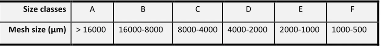
To evaluate the distribution of native and non-native mussel and oyster species scraping samples of the intertidal assemblages were carried out. The density of the bivalve species was estimated using 3 randomly located quadrats (20 × 20 cm) per site and exposition. Once scraped the assemblages were collected into a 500 µm mesh bags, with the aim to retain all the benthic macrofauna. The content of each scraped sample was transferred into a sterile plastic bag, transported in the laboratory and stored at -20°C. The number of individuals of mussel and oyster species in the samples was counted. Individuals were separated into 6 different size class based on Bertasi et al. (2007), using different mesh size sieves (Table 4). The abundance of bivalves in each size class was used to obtain an indication of the population structure of the target species.
Table 4: Sieve mesh size classes utilized. Size classes A B C D E F Mesh size (µm) > 16000 16000-8000 8000-4000 4000-2000 2000-1000 1000-500
2.5. Spatial-temporal variability of settlers
To understand if the species distribution across the 5 sites was related to the settlers rate, the method described by Porri et al. (2006b) was used. From March to July 2017, at each site, 6 plastic scouring pads (MasterClean® polypropylene) as larval collectors were deployed, 3 for each exposure. The pads were attached at the seawall ≈ 1 m apart to metal screws using plastic cable ties (Figure 9). To detect temporal variation of settlers across sites each scouring pad was collected and replaced with a new one every 2 weeks. Each scouring pad removed was placed into a plastic bag with zippers. Once back to the laboratory, collected pads were processed following the protocol described in Porri et al. (2006b) and summarised below and in Table 5. Each pad was agitated in bleach to facilitate the detachment of settlers. The bleach with the released organisms from the pad was sieved through a 75 μm sieve size. The retained settlers were collected from the sieved and stored in absolute ethanol until analysis. Settlers were counted, identified, and sorted out from the other organisms under a stereomicroscope (Nikon SMZ 15000). Given the difficulties in discriminating between the different species by shell morphology (except for individuals > 500 µm), a barcoding approach for the species identification was developed (see section 2.2.5 for details).Table 5: Scouring pad protocol (Porri et al., 2006).
1. Add 9 - 10 ml of bleach per 250 ml of fresh water into a sample bottle; shake well and leave for 5 minutes to soak. 2. Pour the water content of bottle over a 75 µm sieve. 3. Put the washed scouring pad into a 5000 ml bucket. 4. Carefully rinse the sample bottle out over the 75 µm sieve until clean. 5. Cut and unravel the scouring pad into the 5000-ml bucket and rinse it down with a hose/pipe, removing all the debris from the souring pad. Be careful not to splash any water out of the bucket. 6. Pour the water content of the 5000 ml bucket over the 75 µm sieve.
bucket, without splashing any water out of the bucket. 8. Repeat steps 5-7 until the scouring pad is completely clean. 9. Rinse off any tools used (scissors, tweezers etc.) over the sieve. 10. Transfer what is in the sieve to a test tube and add absolute ethanol till the sample in the test tube is completely submerged. Figure 9: Example of scouring pad attached to intertidal zone (photo from S4, north exposition).
2.6. Genetic analysis
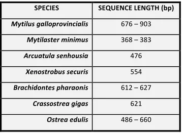
Before starting with the genetic analysis, a bibliography research on National Centre for Biotechnology Information (NCBI, https://www.ncbi.nlm.nih.gov) was carried out to retrieve all the sequence available for the Cytochrome Oxidase subunit I (COI) region of the mitochondrial DNA since it is considered a good barcode to discriminate bivalves. The target species included all the ones retrieved by Abbiati and Ponti (2015, unpublished data). The different length, in base pairs (bp), of the respective target species COI are shown below (Table 6):
Table 6: Length in base pairs (bp) of the COI region regarding the target species. SPECIES SEQUENCE LENGTH (bp) Mytilus galloprovincialis 676 – 903 Mytilaster minimus 368 – 383 Arcuatula senhousia 476 Xenostrobus securis 554 Brachidontes pharaonis 612 – 627 Crassostrea gigas 621 Ostrea edulis 486 – 660
2.6.1. DNA extraction
Different DNA extraction methods were tested to find the best protocol for the extraction of the DNA from the bivalves settlers. The methods used were two: a CTAB protocol with a chloroform washing step and MinElute PCR Purification Kit (Qiagen, Hilden, Germany). This kit has a high sensitivity with low concentrations of DNA (70 b – 4 kb). The protocol provided by (Cilli et al., 2015) was performed using half of the reagent volumes specified. The two methods were tested from 1 to 4 settlers altogether to evaluate their efficiency.2.6.2. PCR amplification protocol
The technique of polymerase chain reaction (PCR) was used to amplify the COI region of each settler. The thermal cycler used was the SimpliAmp Thermal Cycler (Applied Biosystems, Foster City, CA, USA). Several PCR protocols and cycle were explored to find the best amplification yield. The final PCR protocol is shown in Table 7.
Table 7 – PCR mix components.
REAGENTS FINAL VOLUME (µl) ENTERPRISE
H2O sterile nuclease free 2,55 Thermo Fisher Scientific, Waltham, MA, USA MgCl2 1,25 Invitrogen Corp., Carlsbad, CA, USA PCR Reaction Buffer 1,25 Invitrogen Corp., Carlsbad, CA, USA dNTPs 1,25 Promega, Madison, WI, USA Forward Primer 1,25 Macrogen, South Corea Reverse Primer 1,25 Macrogen, South Corea
The primers used were the universal primers LCO1490 (forward) and HCO2198 (reverse) non-degenerated (Folmer 1994) as reported in Table 8: Table 8 – Sequences of forward and reverse primers utilized. FORWARD PRIMER (LCO1490) REVERSE PRIMER (HCO2198) 5’-GGTCAACAAATCATAAAGATATTGG-3’ 5’-TAAACTTCAGGGTGACCAAAAAATCA-3’ The PCR protocol was composed by a preliminary phase of thermic denaturation at 95°C for 3 minutes, followed by 35 cycles of these steps: (i) 95°C for 30 seconds, (ii) 47°C for 30 seconds, (iii) 72°C for 45 seconds. At the end of the 35 cycles, we inserted a 72°C phase for 7 minutes, before the final storage phase of 4°C. The PCR protocol described above was used to amplify the COI region from single settlers. For samples containing 5 or more individuals, a metabarcoding approach was developed in silico but not tested in the thesis.
2.6.3. Agarose gel run
This phase was performed to validate the correct PCR amplification step. The agarose gel was made with 100 ml of TBE (Tris/Borate/EDTA buffer 10x, Thermo Fisher Scientific, Waltham, MA, USA), 1,5 g of CSL-AG500 LE Agarose MultiPurpose Agarose (Cleaver Scientific LTD, Rugby, UK) and 3 µl of GelRed™ Nucleic Acid Stain 10000x in water (Biotium INC, Fremont, CA, USA). Once charged the DNA using 10x Blue Juice ™ Gel Loading Buffer (Invitrogen Corp., Carlsbad, CA, USA), and Sharpmass ™ 100 Plus Ready-to-load DNA Ladder (EuroClone, Milano, Italy), the electrophoresis run was set using the Agagel Midi-Wide horizontal electrophoresis system (Biometra, Göttingen, Germany). After covering with enough 0,5x TBE the gel, the run was set with 90 mV, 75 mAh and for a duration period of 35 minutes.
2.6.4. Sanger sequencing plate preparation
The PCR products were prepared for the sequencing using the ExoSap-IT Cleanup kit (USB Corp., Cleveland, OH, USA), following the protocol provided by the manufacturer. Both strands of DNA were sequenced by Macrogen ® Inc. (Seoul, Korea) using the same primers of the PCR protocol, using MicroAmp optical 96 well Reaction Plate (Applied Biosystems, Foster
City, CA, USA). The sequencing technique chosen was the Sanger sequencing (1975), which uses dideoxide nucleotides (ddNTPs) to obtain the whole sequence of the COI region.
2.7. Statistical analysis
2.7.1. Distribution of sites by environmental parameters
Principal coordinate Analysis (PCoA) using PRIMER v.6 (Clarke and Gorley, 2006) was performed to visualise difference among sites according to their environmental variables (9 variables both chemical and physical, see Table 9). “chart.Correlation” function in the “PerformanceAnalytics” R package (Peterson and Carl, 2014) was used to detect strong correlations or possible skewness between environmental variables. A log(x + 1) transformation was applied to nitrate, nitrite and phosphate concentration to correct right-skewness (Figure 10). Then, PCoA was performed on Euclidean distance matrix calculated from the normalised environmental data (as they were expressed in different scales).
2.7.2. Spatial distribution of native and non-native mussel and oyster species
Differences between sites (Site; 5 random levels = S1, S2, S3, S4 and S5) and Exposition aspect (Exp.; 2 fixed levels = n and s) of native and non-native mussels and oysters were tested using a multivariate permutation analysis of variance (PERMANOVA) with PERMANOVA+ (Anderson and Gorley, 2008) for PRIMER v.6 (Clarke and Gorley, 2006). The PERMANOVA analysis was based on a Bray-Curtis similarity matrix with type III of sum of squares, 9999 permutations and unrestricted permutation of raw data. Spatial distribution was displayed by unconstrained ordination plots using the principal coordinate analysis (PCoA), based on a Bray-Curtis distance matrix calculated from the square root transformed data abundance. A 3-way ANOVAs were used to investigate differences in the distribution of the native and non-native species (nat_inv; 2 fixed levels = nat and no.nat) or mussels (muss; 2 fixed levels = MG and XS), or oysters (oys; 2 fixed levels = OE and CG) across site (site; 5 random levels = S1, S2, S3, S4 and S5) and exposure aspect (exp.; 2 fixed levels = n and s).2.7.3. Relationship between seawall adults and environmental variables
Distance-based linear model (DistLM) (Legendre and Andersson, 1999) analysis was used to identify which of the environmental variables collected described the pattern of mussels and oysters assemblages between sites. Then, environmental variables were transformed and normalised as described above. DistLM analysis was applied on Bray-Curtis similarity matrix of square root abundance data. The analysis was performed using PERMANOVA+ (Anderson and Gorley, 2008) in PRIMER v.6 (Clarke and Gorley, 2006). The Best and Bayesian Information Criterion (BIC) was used as selection procedure and selection criterion respectively (9999 permutations) to find a reduced model that retained only the variables with good explanatory power. Distance-based redundancy analysis (db-RDA) was used to visualise the reduced model obtained. Moreover, vectors showing the direction of increasing abundances of different species along the study sites were superimposed to show highest correlation (Pearson correlation) with the set of environmental variables selected (Anderson and Gorley, 2008).
2.7.4. Settlers spatial-temporal variability analysis
To test differences in the settler’s abundances the temporal factor (Time; 7 random levels = T1, … T7) was added. ANOVA analyses were performed in R software 3.3.1 (R Development Core Team, 2011) using the “gad” function in the “GAD” R-package (Sandrini-Neto and Camargo, 2016). Normality and homogeneity of variance were tested with the “shapiro.test” and the “C.test” functions respectively. When assumptions of normality and homogeneity could not be satisfied, the dependent variable was logarithmically transformed. Significant results were tested by post-hoc pairwise comparisons with the Student-Newman-Keul’s testusing the “snk.test” function.
2.7.5. Relationship between seawall adults and settlers abundances
Coupling between the abundance of settlers scouring pads and adults on artificial walls was investigated. For each temporal survey, the mean values of settlers were correlated with those for adults on the seawall and the Pearson correlation coefficients (r) calculated. Pearson correlation coefficient (r) is considered as follows: (i) light correlation 0 < r < 0.3, (ii) 0.3 < r < 0.7 moderate correlation, (iii) r > 0.7 high correlation.
3. RESULTS
3.1. Environmental variables
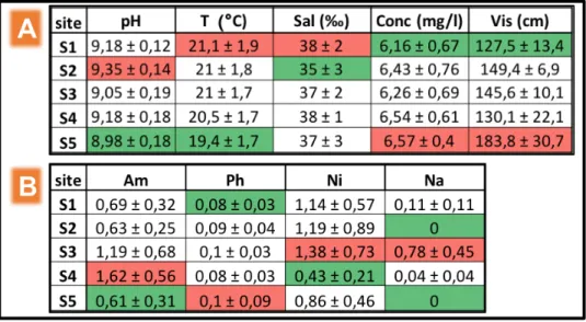
The environmental variables changed across sites in the Ravenna canal-port. pH ranged from 8.98 to 9.35, with a mean value of 9.15 ± 0.16. Sea surface temperature ranged from 19.4 °C to 21.1 °C, averaging 20.6 °C ± 1.76. Mean salinity was 37.1 ‰ ± 2.1, varying from 36.5 ‰ to 38.4 ‰. Oxygen concentration (mg/l) ranged from 6.2 mg/l to 6.6 mg/l, with a mean of 6.4 mg/l ± 0.62. Minimum visibility was 127.5 m, with a maximum of 183.8 m and an average of 147.3 m ± 16.6 (Table 9A). As regards nutrients, Ammonia ranged from 0.61 to 1.62 mg/l, with a mean of 0.95 mg/l ± 0.42. Phosphate ranged from 0.08 to 0.1 mg/l, with an average of 0.09 mg/l ± 0.04. With a mean of 1.00 mg/l ± 0.57, Nitrite varied from 0.43 to 1.38 mg/l. Minimum Nitrate was 0 mg/l, with a maximum of 0.78 mg/l, averaging 0.19 mg/l ± 0.12 (Table 9B).Table 9: Means and relative standard errors of physical variables (Table 1A) and chemical variables (Table 1B) per each site; minimum and maximum values are highlighted in green and in red respectively. pH = Seawater pH T = Sea surface temperature (°C), Sal = Salinity (‰), Conc = Oxygen concentration (mg/l), Vis = Visibility (cm). Am = Ammonia, Ph = Phosphate, Ni = Nitrite, Na = Nitrate (all measures are expressed in mg/l concentrations).
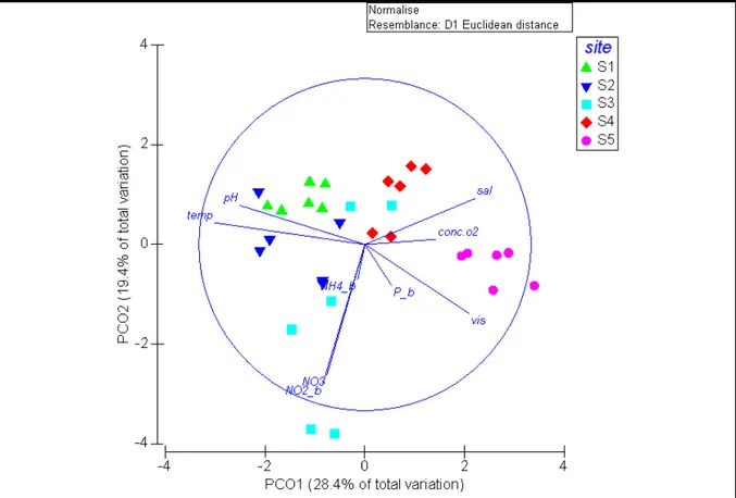
Figure 10: PCoA ordination showing the distribution of sites by the environmental variables. pH = pH; temp = sea surface temperature; sal = salinity; conc.o2 = seawater oxygen concentration; vis = visibility; NO2_b = log + 1 of nitrite concentration; NO3 = nitrate concentration; NH4_b = log + 1 of ammonia concentration; P_b = log + 1 phosphate concentration.
The first axis of the PCoA explained the 28.4 % of the total variation, while the second axis (PC2) explained 19.4% of the total variation. Together, PC1 and PC2 explained the 47.8 % of the total variation. Globally, 6 of the 9 environmental variables showed a high correlation with sites. S5 seemed to group alone respect to the other sites (S1, S2, S3, S4). The isolation of S5 from the other sites looked like being explained by the increasing of visibility and salinity and slightly by oxygen concentration; while seawater pH and temperature increased towards S1, S2, S3 and S4. The S3 is characterized by a high variation of NO3- and NO2- . NH4+
and P seemed not to contribute to the site distribution (Pearson correlation R < 3).
3.2. Changes in abundances of seawall mussels and oysters
3.2.1 Adults samples analysis
The PERMANOVA analysis revealed significant differences between abundances of oysters and mussels across sites and expositions (Table S1; site, pseudo F(df = 4, 20) = 74.81, p < 0.01;
exp, pseudo F(df = 1, 20) = 0.94, p > 0.05; site x exp, pseudo F(df = 4, 20) = 8.81, p < 0.01). The
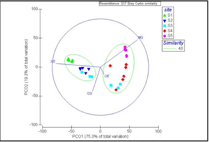
relative PCoA ordination showed these differences (Figure 11). The first two axes explained a total of 94.57 % of the global variability. The first axis accounted for the major part of the variance (75.3 %), and highlighted differences between S1, S2 and S4, S5, reflecting a clear separation between non-native and native species. In particular, native species (M. gigas and O. edulis) increased towards S4 and S5, while non-native species (X. securis and C. gigas) showed an opposite trend in a direction of S2 and S1. The second PCoA axis seemed to discriminate the S3 from the other four sites (19.3 % of explained variation). The S3 is characterised by an increased abundance of the two oyster species (Figure 11).
Figure 11: PCoA of abundances of oysters and mussels across sites and expositions (XS = Xenostrobus securis, CG =
Crassostrea gigas, OE = Ostrea edulis, MG = Mytilus galloprovincialis).
3.2.2. Mussel species distribution
The distribution of M. galloprovincialis (MG) and X. securis (XS) was significantly different across sites and exposition (Figure 12, Table S2).
Figure 12: Differences in the abundance of M. galloprovincialis and X. securis across site and exposition aspect with the relevance of significance values (* < 0.1, ** < 0.01, *** < 0.001). Black and blue asterisks represented significant differences between species and between exposition aspect respectively. M. galloprovincialis was absence in the inner part of the canal-port (S1), while it increased towards the outer part of the port (S5). An appositive trend was observed for X. securis that increased its abundance going to the inner part of the Candiano canal (S1). The two species, showed significant differences in the abundance in sites S1, S2 and S5. In S1 and S5 there were significant differences in the abundance of the same species between north and south exposition aspect (Table S3). The total number of individuals of the two mussel species varied from 1 to 1063 for M. galloprovincialis, and from 3 to 659 for X. securis.
The variation observed between the two mussel species is supported by the rank abundance analysis. The native M. galloprovincialis (Figure 13A) reported a high population structure (with different size class well represented) in S4 and in S5. The main represented size classes were 16000-8000 µm and 8000-4000 µm. The size class 16000 µm was present in all the sites.
The non-native mussel X. securis (Figure 13B), described a les structured population. This species was more abundant in S1 and S2. No individuals belonging to the first size class were observed.
Figure 13: Class-size abundances of target mussel species for each site and exposition aspect, with related mean and standard error. The different size classes chosen were: > 16000 µm (red bars), 16000-8000 µm (green bars), 8000-4000 µm (blue bars), 4000-2000 µm (purple bars). A = Mytilus galloprovincialis; B = Xenostrobus securis.
3.2.3. Oysters species distributions
Figure 14: O. edulis and C. gigas distribution together with the relevance of significance values (** < 0.01, *** < 0.001). Black and blue asterisks represented significant differences between species and between exposition aspect respectively.
The maximum number of oyster retrieved in the wall scraping for each species, O. edulis (OE,) and C. gigas (CG) was 4 individuals. In S1 any oysters were present, while in S5, the only species retrieved was O. edulis. In S2, S3 and S5 main difference in the abundance of the two species were founded. For C. gigas, showed differences in terms of abundance between the two expositions (north and south) at site S2 and site S3.
Unlike mussel species, along the Ravenna canal-port, oysters were represented only by one size class (> 16000 µm) (Figure 15A and 15B). We have the evidence of absence of the non-native species in S5, and the contrary absence of size class (> 16000 µm) (Figure 15A and 15B). We have the evidence of absence of the non-native species in S1. In addition, any oysters were retrieved in S1.
Figure 15: Rank abundance of target oyster species for each site and exposition, with relative mean and standard error. The different size classes chosen were: >16000 µm (red bars), 16000-8000 µm (green bars), 8000-4000 µm (blue bars ), 4000-2000 µm (purple bars). A = Ostrea edulis, B = Crassostrea gigas.
3.2.4. Relationship between environmental variables and adults
When tested individually (Marginal test, Table S4A), sea surface temperature, pH, visibility, salinity and oxygen concentration significantly explained individually the 48 %, 27 %, 23 %, 21 %, 12 % of variability of mussel an oyster species abundances respectively. The other factors (Nitrate, Nitrite, Phosphate and Ammonia seawater concentration) instead did not
modelling the distribution of these bivalves was the sea surface temperature (49 %), while the combination of the environmental parameters (sea surface temperature, oxygen concentration and nitrate) best explaining the overall variation (Overall Best solution, Table S4C). The first axis of dbRDA ordination explained the 88.5 % of fitted, 50.5 % of total variation, while the second axis explained the 11.6 % of fitted, 6.6 % of total variation respectively. The variable mostly related with the dbRDA1 axis was the sea surface temperature (+ 0.942), while the dbRDA2 axis was related with nitrate (+ 0.757) and oxygen concentration (+ 0.616) variables (Figure 16).
Figure 16: Distance-based redundancy analysis (dbRDA) plot showing relationships between the ordination of the sites based on the abundance of target bivalves species and environmental variables. pH = pH; temp = sea surface temperature; conc.o2 = seawater oxygen concentration; NO3 = nitrate concentration; n = north exposition aspect; s = south exposition aspect.
When looking at the plot displaying the different bivalve’s species (Figure 11), X. securis have a positive relationship with the increase of sea surface temperature while M.
galloprovincialis showed an opposite trend. C. gigas and O. edulis showed a slight
Figure 17: Distance-based redundancy analysis (dbRDA)plot showing direction of increasing abundances of target bivalves species across the study sites. MG = M. galloprovincialis; XS = X. securis; OE = O. edulis; CG = C. gigas. Chi sono n e s? exposition?
3.2.5. Settlers spatial-temporal variability
An example of settlers obtained from the scouring pads are shown in Figure 18.
Settlers abundances ranged from 1 (several sites and times) to 1759 individuals (T6, site S2, south exposition). These abundances varied significantly across sites and times (Table S5, Figure 19).
Figure 19: Temporal settler’s abundance in each site and exposition aspect. Blue and red points indicate north and south exposition respectively. Values are mean values and standard errors. Original data were transformed (log + 1). A = site S1, B = site S2 ,C = site S3, D = site S4, E = site S5. In particular, settler’s abundance increased across time in site S1, S2 and S3, reaching their maximum during June and July, while S5 showed a decrease of settlers through time. S4 did not show a clear trend in the abundance of settlers across time.
3.2.6. Correlation between settlers and adult abundance
There was a light correlation between adults and settlers. The R2 value was 0.34 (Figure 18A). However, data exploration revealed the presence of three outlier values in site S2, south exposition (Figure 20). Removing these values, the correlation increased of R2 = 0.45
Figure 20: Correlation between mean abundance of adult bivalves species and mean abundances of settlers. Global Pearson correlation R2 = 0.34. Outlier values are circled in black. Figure 21: Correlation between mean abundance of adult bivalves species and mean abundances of settlers, removing S2 outlier values. Global Pearson correlation R2 = 0.45.
3.3. DNA extraction and amplification from a single settler
The DNA extraction protocol firstly used was based on Phenol-Chloroform procedure. The several attempts with this technique did not show any positive results using a single settler, as the quantity of material to extract the DNA was too low (settler’s dimensions lower than200 µm). Extraction of samples contained ≤ 4 settler’s individuals resulted to have a proper DNA extraction, having a clear band in the agarose gel post-extraction run.
This methodological comparison showed a high sensitivity (75%) of the MinElute PCR extraction kit to extract DNA from single bivalve settlers.
With this extraction was possible to amplify a region of the COI up to 900 pb. The PCR protocol was performed and adapted, starting from Folmer et al (1994). Trying different MgCl2 and primers concentrations, 15/20 organisms were amplified properly (Figure 22). Figure 22: Gel electrophoresis (1.5 Agarose + GelRed) after PCR with annealing 47°C 30” (35 cycles). Marker was 100 bp. Is known from literature that the COI sequence for Mytilus galloprovincialis ranges from 676 to 903 bp. Xenostrobus securis has a COI sequence of 383 bp, Crassostrea gigas 621 bp and Ostrea edulis 486 – 660 bp. Samples 2, 3, 8, 12, 16, 18, 20 have a clear band between 800 and 900 bp.
4. DISCUSSION
In this thesis, I explored the distribution and abundance of 2 native (M. galloprovincialis, O.
edulis) and 2 non-native (X. securis, C. gigas) bivalve species growing on the artificial
seawalls of the Ravenna channel-port. Moreover, I observed their distribution was related to specific environmental variables and/or to the abundance of settlers reaching these seawalls directly. The main results showed that the distribution of native intertidal bivalve species decreases as going inland. On the other hand, the gradual loosing of open sea conditions led to have an increasing in non-native species abundance on the canal-port seawalls. This population gradient is mainly linked with the increasing of sea surface temperatures, with mean differences between the most internal and external site of about 2 °C. Likewise, the spatial-temporal supply of settlers reaching the seawall was moderately related to the abundance of the adults founded on the canal-port seawalls.
Most of the environmental variables changed along the Ravenna canal-port and explained a consistent part of the variability in abundance of the four target bivalve species. Changes in the environmental variables seems to be related to the morphological characteristics of the canal-port. Sites located near the canal-port doorway are more affected by open sea conditions, while the inland sites have characteristics similar to those of closed water basin. In particular, the site S5, that is the closest to the open sea, showed a high influence of the salted and O2 rich waters supplied by the Adriatic Sea. The phosphate content was also
higher in S5 compared to the other sites, possibly due to water contributions of Pialassa Baiona or the Po river waters (Airoldi et al., 2016). Going towards the internal part of the canal-port (S3, S2, S1), I observed an increase in pH and nutrients concentration. A pH major than 9.0, nutrients increasing and lowest salinity should be related to the presence of urban drains in this area (Airoldi et al., 2016) (http://www.provincia.ra.it/). Usually urban drains are freshwater-enriched, and can contain alkaline soaps and other types of pollutant (Us Epa, 2003).
Sea surface temperature increased going from the outer to the inland part of the canal-port. This pattern could be attributable to low water exchange rate and/or to a major evaporation in the inland part of the canal. Sea surface temperature was the main drivers of species
presence in the inland part of the canal-port (high sea surface temperature and salinity), while the native species, M. galloprovincialis and O. edulis, prefer environmental conditions similar to those of the open sea (higher O2 concentration and lower seawater temperature). This result is in accordance with the observation of Astudillo et al. (2017), that report how X. securis is able to tolerates high seawater temperature and high salinity. Moreover, the site S3 placed approximately in the middle of the canal-port, evidenced the presence of both native and non-native species. This area could represent an ecotone, acting as a transition zone for the distribution of both native and non-native species. In this area an interspecific space competition can occur among the different mussel and oyster species (Russo, 2001). In fact, personal field observations highlight how X. securis tends to grow in the upper part of the sampled intertidal zone while M. galloprovincialis was present in the lower portion of our scraped areas. This observation leads to hypothesise that X. securis not only prefer higher temperature but it can also tolerate other stressors related to the air exposition (e.g. solar irradiance, dry-out).
Native and non-native species were differently abundant in the two exposition aspects investigated. We hypothesise that these differences could be explained by possible variation in solar irradiance and/or water circulation present at each site.
Bivalves settlers abundances showed a significant spatial and temporal variability. In particular, the inner and outer parts of the canal-port seem to receive different amounts of settlers across time. The outer part, characterised by a high abundance of M.
galloprovincialis, present the maximum peak of settlers in March. This led to hypothesize
that these settlers belong to M. galloprovincialis, as it was observed that the spawning period of this species occurs from November to March (Ceccherelli & Rossi 1984). Conversely, the inland part of the canal-port presents a peak of settlers abundance in May, when seawater temperatures are higher, suggesting that these settlers could belong to X.
securis (Wilson, 1969). Otherwise, these settlers may also belong to the two oysters target
species retrieved. In fact, C. gigas and O. edulis present spawning overlapped spawning periods going from the end of May till the end of July (Massapina et al., 1999; Bataller et al., 2006).
The presence of adult bivalves on the artificial seawalls of the canal-port was moderately related to the abundance of settlers. However, due to the lack of settler’s identification, it
was not possible to carry out a correlation between adults and settlers of the same species. In this perspective, we identified specific settlers DNA extraction and amplification protocols from single settler individuals. The further step will be the development of a metabarcoding protocol to identify the species in a settlers pool.
5. CONCLUSIONS
This study increases the knowledge about native and non-native species interaction in harbour environment. In fact, the special distribution of native and non-native species seems to depend by the biological characteristics of the single species. Here the abundance of non-native species, compared to the native ones, increases together with the intensification of human-related pressures (Megina et al., 2016). In particular, propagule pressure enhanced by larval persistence in the water column seems to increase where seawater circulation and exchange is limited (Rivero et al., 2013). Future experiments should be carried out to deepen the knowledge of this anthropogenic environment. For example, will be interesting to: (i) increase the number of environmental variables including hydrodynamics and urban discharge to better understand the water cycling inside the canal-port and (ii) extend to 1 year the duration of the experiment to have a broader comprehension of temporal changes in the abundance of settlers. Moreover, the addition of the analysis of the larval abundance in the water will help to understand better the dynamics that lead to the seawall colonisation. In this perspective, the addition of metabarcoding approach could help not only to identify at what species belong the larval/settlers but also to determine if the abundance of the adults is related to the propagule pressure.
6. REFERENCES
Airoldi, L., 2003. The effects of sedimentation on rocky coast assemblages. Oceanogr. Mar. Biol. 41, 161–236. https://doi.org/10.1201/9780203180570.ch4 Airoldi, L., Balata, D., Beck, M.W., 2008. The Gray Zone: Relationships between habitat loss and marine diversity and their applications in conservation. J. Exp. Mar. Bio. Ecol. 366, 8–15. https://doi.org/10.1016/j.jembe.2008.07.034 Airoldi, L., Bulleri, F., 2011. Anthropogenic disturbance can determine the magnitude of opportunistic species responses on marine urban infrastructures. PLoS One 6. https://doi.org/10.1371/journal.pone.0022985 Airoldi, L., Crowe, T.P., Russell, R., 2009. Functional and Taxonomic Perspectives of Marine Biodiversity. Mar. Hard Bottom Communities Patterns, Dyn. Divers. Chang. 375–390. https://doi.org/10.1007/978-3-540-92704-4 Airoldi, L., Ponti, M., Abbiati, M., 2016. Conservation challenges in human dominated seascapes: The harbour and coast of Ravenna. Reg. Stud. Mar. Sci. 8, 308–318. https://doi.org/10.1016/j.rsma.2015.11.003 Airoldi, L., Turon, X., Perkol-Finkel, S., Rius, M., 2015. Corridors for aliens but not for natives: effects of marine urban sprawl at a regional scale. Divers. Distrib. 21, 755–768. https://doi.org/10.1111/ddi.12301 Anderson, M., Gorley, R., 2008. PERMANOVA for PRIMER Guide to Software and Statistical Methods. Astudillo, J.C., Bonebrake, T.C., Leung, K.M.Y., 2017. The recently introduced bivalve Xenostrobus securis has higher thermal and salinity tolerance than the native Brachidontes variabilis and established Mytilopsis sallei. Mar. Pollut. Bull. 118, 229–236. https://doi.org/10.1016/j.marpolbul.2017.02.046 Bacchiocchi, F., Airoldi, L., 2003. Distribution and dynamics of epibiota on hard structures for coastal protection 56, 1157–1166. https://doi.org/10.1016/S0272-7714(02)00322-0 Barbieri, M., Maltagliati, F., Di Giuseppe, G., Cossu, P., Lardicci, C., Castelli, A., 2011. Newbiotopes of the western Mediterranean provide evidence of its invasive potential. Mar. Biodivers. Rec. 4, e48. https://doi.org/10.1017/s175526721100042x Bataller, E., Burke, K., Ouellette, M., Maillet, M.-J., 2006. Evaluation of spawning period and spat collection of the northernmost popuulation of European oysters (Ostrea edulis L.) on the Canadian Atlantic coast. Beck, M.W., Brumbaugh, R.D., Airoldi, L., Carranza, A., Coen, L.D., Crawford, C., Defeo, O., Edgar, G.J., Hancock, B., Kay, M.C., Lenihan, H.S., Luckenbach, M.W., Toropova, C.L., Zhang, G., Guo, X., 2011. Oyster Reefs at Risk and Recommendations for Conservation, Restoration, and Management. Bioscience 61, 107–116. https://doi.org/10.1525/bio.2011.61.2.5 Bertasi, F., Colangelo, M.A., Abbiati, M., Ceccherelli, V.U., 2007. Effects of an artificial protection structure on the sandy shore macrofaunal community: The special case of Lido di Dante (Northern Adriatic Sea). Hydrobiologia 586, 277–290. https://doi.org/10.1007/s10750-007-0701-y Bownes, S., Barker, N.P., McQuaid, C.D., 2008. Morphological identification of primary settlers and post-larvae of three mussel species from the coast of South Africa. African J. Mar. Sci. 30, 233–240. https://doi.org/10.2989/AJMS.2008.30.2.3.553 Branch, G.M., Nina Steffani, C., 2004. Can we predict the effects of alien species? A case-history of the invasion of South Africa by Mytilus galloprovincialis (Lamarck). J. Exp. Mar. Bio. Ecol. 300, 189–215. https://doi.org/10.1016/j.jembe.2003.12.007 Bulleri, F., Airoldi, L., 2005. Artificial marine structures facilitate the spread of a non-indigenous green alga, Codium fragile ssp. tomentosoides, in the north Adriatic Sea. J. Appl. Ecol. 42, 1063–1072. https://doi.org/10.1111/j.1365-2664.2005.01096.x Bulleri, F., Chapman, M.G., 2004. Intertidal assemblages on artificial and natural habitats in marinas on the north-west coast of Italy. Mar. Biol. 145, 381–391. https://doi.org/10.1007/s00227-004-1316-8 Bulleri, F., Chapman, M.G., Underwood, A.J., 2005. Intertidal assemblages on seawalls and vertical rocky shores in Sydney Harbour, Australia. Austral Ecol. 30, 655–667. https://doi.org/10.1111/j.1442-9993.2005.01507.x
Carlton, J.T., 1987. Patterns of Transoceanic Marine Biological Invasions in the Pacific-Ocean. Bull. Mar. Sci. 41, 452–465. Ceccherelli, V.U., Rossi, R., 1984. Settlement, growth and production of the mussel Mytilus galloprovincialis. Mar. Ecol. Prog. Ser. 16, 173–184. https://doi.org/Doi 10.3354/Meps016173 Chapman, M.G., 2003. Paucity of mobile species on constructed seawalls: Effects of urbanization on biodiversity. Mar. Ecol. Prog. Ser. 264, 21–29. https://doi.org/10.3354/meps264021 Cilli, E., De Fanti, S., Quagliariello, A., Sarno, S., Serventi, P., Traversari, M., Zedde, A., Luiselli, D., Gruppioni, G., 2015. Genetic analysis of the population of Roccapelago - Modena (Italy) (16th - 18th c.). ArchaeoAnalytics. Chromatogr. DNA Anal. Archaeol. 247–254. Clark, G.F., Johnston, E.L., 2009. Propagule pressure and disturbance interact to overcome biotic resistance of marine invertebrate communities. Oikos 118, 1679–1686. https://doi.org/10.1111/j.1600-0706.2009.17564.x Clarke, K.R., Gorley, R.N., 2006. PRIMER v6: User Manual/Tutorial. Prim. Plymouth UK. https://doi.org/10.1111/j.1442-9993.1993.tb00438.x Clarke Murray, C., Pakhomov, E.A., Therriault, T.W., 2011. Recreational boating: A large unregulated vector transporting marine invasive species. Divers. Distrib. 17, 1161–1172. https://doi.org/10.1111/j.1472-4642.2011.00798.x Crossland, C.J., Baird, D., Ducrotoy, J.-P., Lindeboom, H., Buddemeier, R.W., Dennison, W.C., Maxwell, B.A., Smith, S. V., Swaney, D.P., 2005. The Coastal Zone — a Domain of Global Interactions. Coast. Fluxes Antropocene 1–37. https://doi.org/10.1007/3-540-27851-6_1 Dafforn, K.A., Glasby, T.M., Johnston, E.L., 2012. Comparing the invasibility of experimental “reefs” with field observations of natural reefs and artificial structures. PLoS One 7, 1– 16. https://doi.org/10.1371/journal.pone.0038124 Dafforn, K.A., Glasby, T.M., Johnston, E.L., 2009. Links between estuarine condition and spatial distributions of marine invaders. Divers. Distrib. 15, 807–821.