Corso di Laurea Magistrale in Ingegneria Civile
AN ENGINEERING APPROACH TO
THE MULTISCALE MODELING OF THE
LYMPHATIC SYSTEM
Relatore: Prof. Ing. Riccardo Sacco
Correlatore: Prof. Ing. Giovanna Guidoboni
Correlatore: Ing. Raul Pirovano
Tesi di laurea Magistrale di:
Nicholas Mattia Marazzi 883144
Anno accademico 2017/2018
Ringraziamenti
Desidero innanzitutto ringraziare il Professor Sacco. Gli spunti di riflessione e l’interesse suscitato dalle Sue lezioni sono state la spinta ad affrontare questo cammino di tesi e spero un giorno di poter fare tesoro dei preziosi insegnamenti ricevuti in questi mesi.
Vorrei ringraziare profondamente Giovanna. La tua guida scientifica e umana è stata per me un fondamentale riferimento e mi auguro di poter continuare ad apprendere con la stessa passione con cui mi hai seguito e accompagnato nelle sfide di questa ricerca.
Un ringraziamento va a tutto lo staff di XC-engineering, che ho avuto la fortuna di incontrare durante il tirocinio in cui si è ulteriormente sviluppato il presente elaborato. Vorrei in particolare ringraziare Raul, che mi ha affiancato e guidato alla conoscenza di FLOW-3D dedicando numerose ore allo sviluppo della tesi.
Questa tesi rappresenta il momento finale di un percorso iniziato cinque anni fa. Tale cammino non sarebbe stato possibile senza il supporto dei miei genitori, coloro che hanno vissuto più da vicino quest’avventura sostenendomi ed aiutandomi in ogni situazione. Spero un giorno di potervi restituire una piccola parte di tutto quello che avete fatto per me. Un ringraziamento speciale va a mia sorella Arianna, la persona che mi ha aiutato a ritrovarmi nei momenti più intensi e che continua ad insegnarmi con enorme semplicità la leggerezza delle emozioni. Vorrei che il giorno della laurea fosse presente mio nonno Oreste, la persona che con una frase mi ha fatto capire più di quanto avessi cercato di comprendere per anni. Alla nonna Angela, che tante volte mi ha aspettato e sopportato nei pomeriggi di studi con la sua incredibile gioia e gentilezza. Ai nonni Anna ed Arturo, con cui 18 anni fa muovevo i primi passi alle scuole elementari e che ancora sono vicini a me in ogni momento e in ogni nuova sfida.
Abstract
The lymphatic system constitutes a one-way transport route that operates in conjunction with the cardiovascular system. Its primary function is to maintain overall fluid balance in the human body. In this thesis, we develop two mathematical models, based on fluid-dynamic principles, to characterize the role of the lymphatic system in regulating fluid homeostasis. Although the lymphatic system has a vital role in human health, several mechanisms of this system still need to be elucidated.
Our current work is motivated by this limited knowledge as well as the repercussions of impaired lymphatic function, which can lead to pathological conditions such as lymphedema or tumor metastases. Mathematical models can be used as a virtual laboratory where hypotheses can be tested to advance the quantitative understanding of the lymphatic system.
In the first part of this thesis, we develop a lumped parameter model to simulate fluid balance in the human body. The challenges in the design of this model stem from the uncertainty affecting the physiological knowledge of the regulatory mechanisms of the lymphatic system. Thus, our virtual laboratory offers the possibility of formulating different hypotheses to verify the impact of the lymphatic system on a large scale. The proposed formulation reproduces the main features of the cardiovascular system and has the novelty of embedding both the filtration process and the lymphatic system into a systemic computational framework. Moreover, the model emphasizes the systemic importance of a component of the lymphatic system, known as lymphangions, in the controlled transport of fluid that the lymphatic system must accomplish to maintain homeostasis.
In the second part of the thesis, we analyze the behavior of the lymphangions at a finer scale resolution. To this purpose, we develop a CFD simulation with the commercial software FLOW-3D aimed at studying the fluid-dynamic behavior of this component. We analyze two different configurations. Initially, we studied a single lymphangion and highlight a tight relation between the time-rate of change of pressure stems and valve dynamics. Then, we study a scenario composed of several lymphangions with which we examined the fluid-dynamic quantities in a lymphangions chain and provide a theoretical explanation to justify the observed behavior.
Il sistema linfatico costituisce una via di trasporto ad un solo verso che opera in collaborazione con il sistema cardiovascolare. La funzione principale di questo sistema è il mantenimento del volume ematico. In questa tesi vengono proposti due modelli matematici, basati su principi fluidodinamici, per la caratterizzazione del ruolo del sistema linfatico nella regolazione dell'omeostasi dei fluidi.
Il nostro lavoro attuale è motivato dalla limitata conoscenza dei meccanismi fisiologici dello stesso sistema e dalle ripercussioni di una funzionalità linfatica alterata, che può portare all’insorgenza di patologie come linfedema o metastasi tumorali. In tal senso, i modelli matematici possono essere utilizzati come un laboratorio virtuale in cui è possibile testare ipotesi per far aumentare la comprensione quantitativa del sistema linfatico.
Nella prima parte di questa tesi, viene sviluppato un modello a parametri concentrati per simulare il bilancio di fluidi nel corpo umano. La complessità nella definizione quantitativa di questo modello deriva dall'incertezza riguardo i meccanismi regolatori del sistema linfatico. Pertanto, il laboratorio virtuale offre la possibilità di formulare diverse ipotesi per verificare l'impatto del sistema linfatico su larga scala. Il modello proposto descrive le principali caratteristiche del sistema cardiovascolare, del processo di filtrazione e del sistema linfatico in un quadro computazionale sistemico. Questo modello enfatizza l'importanza sistemica di un componente del sistema linfatico, noto come linfangione, nel trasporto controllato del fluido che il sistema linfatico deve realizzare per mantenere l'omeostasi nel corpo umano. Nella seconda parte della tesi viene analizzato il comportamento dei linfangioni ad una scala locale tridimensionale. A questo scopo, viene sviluppata una modello numerico CFD con il software commerciale FLOW-3D finalizzata allo studio del comportamento fluidodinamico di questo componente. Si sono considerate due diverse configurazioni. Inizialmente si è sviluppata una simulazione ad un unico linfangione con la quale si è evidenziato la dinamica delle pressioni e del movimento delle valvole. A partire dall’osservazione di questo modello, si sono simulate più linfangioni. E’ stato così possibile osservare comportamento fluidodinamico in questa condizione e si è fornita una spiegazione teorica del comportamento osservato.
Contents
RINGRAZIAMENTI ... I
ABSTRACT ... III
SOMMARIO ... IV
CONTENTS ... V
LIST OF FIGURES ... VIII
LIST OF TABLES ... XII CHAPTER 1
INTRODUCTION ... 1
1.1AN INTERDISCIPLINARY APPROACH TO THE MODELLING OF THE LYMPHATIC SYSTEM ... 1
1.2LYMPHATIC SYSTEM ... 3
1.2.1 Tasks of the lymphatic system ... 4
1.2.2 Lymphatic vascular system ... 5
1.2.3 Physiology of the lymphatic system ... 6
1.3LYMPHATIC SYSTEM IN DISEASES ... 7
1.3.1 Lymphedema ... 7
1.3.2 Metastases ... 8
1.3.3 Immune system disfunction ... 8
CHAPTER 2 GOVERNING EQUATIONS ... 9
2.1LUMPED PARAMETER MODEL ... 10
2.1.1 One-dimensional conservation equation ... 10
2.1.2 Zero-dimensional equation ... 12
2.1.3 Fluid electric analogy... 13
... 19
3.1LUMPED PARAMETER MODELING OF FLUID BALANCE IN THE HUMAN BODY ... 19
3.1.1 Structure of the model ... 20
3.1.2 Single and multi-compartment models of arterial and venous trees ... 21
3.2LUMPED PARAMETER DESCRIPTION OF THE HEART AND ITS CONTRACTILE PROPERTY ... 25
3.2.1 Representation of the cardiac cycle through the PV loop ... 25
3.2.2 Theory of time-varying elastance ... 27
3.2.3 Lumped parameter description of the heart ... 30
3.2.4 Mathematical description of the time-varying elastance ... 33
3.3LUMPED PARAMETER MODEL OF THE CARDIOVASCULAR SYSTEM IN A PHYSIOLOGICAL HEALTHY SITUATION 36 3.3.1 Description and development of Avanzolini’s model ... 36
3.3.2 Governing equation ... 39
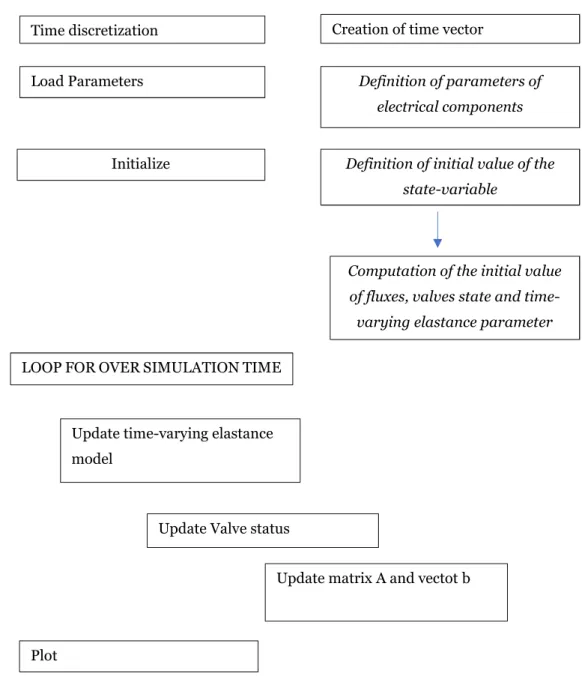
3.3.3 Implementation and system resolution with Matlab and Open Modelica ... 41
3.4FILTRATION PROCESS AND INTERSTITIAL SPACE ... 46
3.4.1 Starling’s law and filtration process ... 46
3.4.2 Electric representation of the filtration process in healthy condition ... 49
3.4.3 Interstitial space and its electric representation ... 51
CHAPTER 4 LUMPED EQUIVALENT MODELING OF THE LYMPHATIC SYSTEM ... 53
4.1LUMPED PARAMETER DESCRIPTION OF THE LYMPHATIC SYSTEM ... 53
4.1.1 A review of lymphangion modeling ... 55
4.1.2 Lumped model of the lymphangion ... 58
4.1.3 Lumped parameter modelling of lymphangion contractility based on Avanzolini time-varying elastance ... 59
4.2INITIAL LYMPHATIC AND THE INTERSTITIAL SPACE ... 62
4.2.1 Connection between lymphatic and interstitial space based on passive elements ... 63
4.2.2 Adding a current source ... 68
4.3RESULTS OF THE MODEL ... 71
4.3.1 Results ... 71
4.3.2 Objective and next modeling directions to further develop the lumped parameter model ... 76 CHAPTER 5
5.1.2 FLOW-3D grid and the FAVORTM method ... 80
5.1.3 Governing equation in FLOW-3D ... 81
Momentum balance ... 83
5.2MATHEMATICAL MODELING OF A LYMPHANGION ... 83
5.2.1 Description of reference article ... 84
5.2.2 Definition of the model ... 85
5.2.3 Challenges and assumptions of the numerical model of a lymphangion ... 85
5.3DEFINITION OF THE NUMERICAL MODELLING WITH FLOW-3D ... 88
5.3.1 GMO model ... 88
5.3.2 Numerical model of the lumped lymphangion with FLOW-3D ... 89
5.3.3 Valve modeling ... 95
5.3.4 Numerical parameters of the simulation ... 96
5.3.5 Mesh assessment ... 96
5.4SIMULATION RESULTS FROM THE 3D MODELLING OF AN EQUIVALENT LYMPHANGION ... 100
5.4.1 Description of pressure behavior ... 100
5.4.2 Valve’s movements ... 104
5.4.3 Improvements of the simulation ... 105
CHAPTER 6 SIMULATION OF A CHAIN OF LYMPHANGIONS ... 110
6.1FEATURES OF A SIMULATION OF A CHAIN OF A LYMPHANGIONS IN FLOW-3D ... 110
6.1.1 Set-up of the simulation ... 111
6.1.2 Valve movement hypothesis ... 112
6.2CALIBRATION OF THE PARAMETERS OF VALVE OPENING AND TIME DELAY ... 115
6.2.1 Opening angle in the new simulation ... 115
6.2.2 Calibration of time delay parameter ... 118
6.2.3 Parameters of the simulation ... 122
6.3RESULTS ... 123
6.3.1 Comparison between experimental and numerical curve ... 123
6.3.2 Pressure and volume flow rate behaviour in the lymphangion chain... 124
6.3.3 Boundary condition dependency ... 129
CHAPTER 7 CONCLUSIONS AND FUTURE PERSPECTIVES ... 133
Figure 1.1 Conceptual structure of the problem of interest 2 Figure 1.2 Lymphoid organs in the human body 3 Figure 1.3 Schematic representation of the lymphatic system 4
Figure 1.4 Lymphatic capillaries 5
Figure 1.5 Lymphangion 5
Figure 1.6 Relationship between the cardiovascular and the lymphatic system 6 Figure 1.7 Lymph flow pathway from the interstitial space to the subclavian vein 7 Figure 2.1 Cardiovascular and lymphatic system 9
Figure 2.2 Compliant tube 10
Figure 2.3 Capacitor 14
Figure 2.4 Resistor 14
Figure 2.5 Inductor 15
Figure 2.6 Computational domain Ω and partition 𝜁 16 Figure 2.7 The element K and outward normal 17 Figure 3.1 Block diagram of the proposed model of human fluid balance 20 Figure 3.2 Cardiovascular and Lymphatic system 21
Figure 3.3 2-element WK model 22
Figure 3.4 3-element WK model 22
Figure 3.5 4-element WK 22
Figure 3.6 RLC combination 23
Figure 3.7 Lumped parameter representation of the venous system 24 Figure 3.8 Cardiac Pressure-Volume Loop 25 Figure 3.9 Graphical representation of the EDPVR 26 Figure 3.10 ESPVR and EDPVR in the PV plane 27 Figure 3.11 Time-varying elastance concept from [28] 27 Figure 3.12 ESPVR and EDPVR in the time-varying elastance model 28 Figure 3.13 Time rate of change of elastance in the PV plane during systole and diastole 29 Figure 3.14 Activation function of the time-varying elastance 29
Figure 3.20 Electric analog of left ventricle (from [17])based on time-varying elastance 34 Figure 3.21 Lumped parameter model of the cardiovascular system 36 Figure 3.22 Physiological compartments described in the model of the cardiovascular system 37 Figure 3.23 Lumped parameter model of the cardiovascular circulation comprising capillary
and venules
38
Figure 3.24 Connector and component in OpenModelica 42 Figure 3.25 Connection between two resistors in Open Modelica 42 Figure 3. 26 Diode in OpenModelica 43 Figure 3.27 Computed time-rate of change of pressure in large arteries 44 Figure 3.28 Computed time-rate of change of pressure in veins 45 Figure 3.29 Computed time-rate of change of pressure in large arteries in capillaries and
venules
45
Figure 3.30 Pressure in the cardiovascular system 46 Figure 3. 31 Graphical representation of Starling’s Law 48 Figure 3.32 Trans-endothelial filtration process 49 Figure 3.33 Lumped equivalent compartment of the capillary 50 Figure 3. 34 Electrical equivalent of the filtration process 50
Figure 3.35 Interstitial space 51
Figure 3.36 Interstitial compliance 52 Figure 4.1
Scheme of human fluid balance
54Figure 4.2
Lymph flow pathways
54Figure 4.3 Lymphangion 55
Figure 4.4 Lumped parameter model of a lymphangion (from [33]) 55 Figure 4. 5 Lumped parameter model of a lymphangion (from [34]) 56 Figure 4.6 Model of a lymphangion from Gajani [32] 57 Figure 4. 7 Model of a lymphangion proposed by [23] 58 Figure 4.8 P-V loop in the lymphangions (from[39]) 59 Figure 4.9 Isovolumic pressure in the heart 60 Figure 4.10 time rate of change of pressure inside a lymphangion 60 Figure 4.11 Connection of the lymphatic system with the cardiovascular space lumped
parameter model of fluid balance with a passive connection between the microcirculation and the cardiovascular system
62
Figure 4.12 lumped parameter model of fluid balance with a passive connection between the microcirculation and the cardiovascular system
63
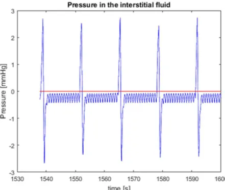
Figure 4.13 Inlet valve of the lymphangions compartment 64 Figure 4.14 Time-rate of change of pressure in the lymphangion compartment 65 Figure 4.15 Effect of RINT on the interstitial pressure 67 Figure 4.16 Effect of RPOST on the interstitial pressure 69
Figure 4.19 process of lymph formation 70 Figure 4.20 time of rate of change of pressure in the large arteries in m=1…18 subsequent
cardiac cycles
72
Figure 4.21 physiological expected aortic pulse pressure 72 Figure 4.22 time of rate of change of pressure in the capillaries in m=1…18 subsequent cardiac
cycles
73
Figure 4. 23 time rate of change of pressure into the interstitium 73 Figure 4.24 time rate of change of pressure in the interstitial space, in the lymphatic system and
the capillaries
74
Figure 4.25 hysteresis loop in the lymphangion 75 Figure 4.26 Comparison between pressure in the interstitial space and flow into the lymphatic
system
76
Figure 4. 27 schematic description of the suction effect 77 Figure 5. 1 :Structure of a CFD software 80 Figure 5. 2 Mesh discretization with FAVORTM 81 Figure 5.3 Experimental set-up of the lymphangion chain described in [7] 84 Figure 5.4 pressure and diameter experimentally measured from [7] 85 Figure 5. 5 geometry of the lymphangion at the end of contraction phase 86 Figure 5. 6 geometry of the lymphangion at the end of diastole phase 86 Figure 5.7 Confocal images of a lymphangion valve 87 Figure 5. 8 valves at the end of systole and in a closed state 87 Figure 5.9 Rendering in FLOW-3D of the lymphangion geometry in the initial condition 90
Figure 5.10 Reference System 90
Figure 5.11 Discretization of the numerical domain to compute discharge 91 Figure 5.12 Time rate of change of discharge computed with Matlab 93 Figure 5.13 Rendering of a lymphangion exploiting the assumption of axial-symmetry 94 Figure 5.14 comparison between experimental and numerical time-diameter curve 95 Figure 5. 15 Moving flange of valve 95 Figure 5.16 Uniform mesh with cell dimension 2.5 e-4 97 Figure 5.17 Time rate of change of pressure with an opening angle of 18.5° 97 Figure 5.18 Outlet volume flow rate 98
Figure 5.24 Pressure comparison in different location inside the lymphangion 102
Figure 5.25 End-systolic phase 103
Figure 5. 26 Valve dynamic 105
Figure 6. 1 experimental set-up of the lymphangion chain described in [7] 111 Figure 6.2 Simulation of a chain of lymphangion in FLOW-3D 111 Figure 6.3 Time-diameter curve of five lymphangions with Td = 0.5 𝑠 112 Figure 6.4 Time-diameter curve of 1st and 2ndlymphangions with Td = 0.5 𝑠 113 Figure 6.5 time rate of change of diameter at the end-diastolic instant of the first lymphangion 113 Figure 6.6 Ideal pressure drop in a lymphangion chain 115 Figure 6.7 Mesh configuration in valve cross section an opening angle of 27° and 37° 116 Figure 6.8 Outlet volume flow rate of the first lymphangion with 2 different maximum
opening angle of valves (27° and 37°)
117
Figure 6.9 comparison of time rate of change of pressure varying the opening angle of valves 117 Figure 6.10 Comparison of time rate of change of pressure with different time delay 118 Figure 6.11 flow rate crossing the first lymphangion with Td=0.5 and Td=0 120 Figure 6.12 flow rate crossing the fifth lymphangion with Td=0.5 and Td=0 120 Figure 6.13 time rate of change of pressure with Td=0, Td=0.05 121 Figure 6.14 Comparison of time rate of change of pressure recorded experimentally with the
simulated one with Td=0.15 and Td=0.05
122
Figure 6.15 comparison between the time rate of change of pressure recorded experimentally and the numerical results
123
Figure 6.16 comparison between the time rate of change of pressure of the model of the equivalent lymphangion and the one of a lymphangion chain
124
Figure 6.17 time rate of change of pressure inside the lymphangion chain 125 Figure 6.18 theoretical description of pressure drop behavior throughout the lymphangion
chain in systole
1265
Figure 6.19 theoretical description of pressure drop behavior throughout the lymphangion chain in diastole
126
Figure 6.20 volume flow rate throughout the lymphangion chain 128 Figure 6.21 velocity field and streamlined at t=1.740 s 128 Figure 6.22 velocity field and streamlined at t=2.520 s 128 Figure 6. 23 boundary condition dynamic corresponding to the minimum diameter of the first
lymphangion
129
Figure 6.24 boundary condition dynamic corresponding to the minimum diameter of the second lymphangion
130
Figure 6.25 boundary condition dynamic at t=2.45 s. 131
Figure 7.1 lymph flow pathways 133
Table 3.1 :Pressure in arterial and venous trees from [22] 37 Table 3.2: value of parameter of lumped model of cardiovascular system 40 Table 3. 3: Matlab
algorithm
to solve the proposed lumped parameter model ofthe cardiovascular system
41
Table 4.1: Parameter value of the proposed lumped parameter model of the 65
Table 4. 2: 66
Table 4. 3: calibration of resistance value in the passive configuration 66 Table 4.4: calibration of resistance value in the passive configuration 67 Table 4. 5: Parameter value of the resistance in the model configuration with a current
source
69 Table 5.1: Matlab code to compute discharge 92 Table 5.2: evaluation of Reynolds number 93 Table 6.1: Valves’ movement scheme between t0 and t1 114 Table 6.2: General valves’ movement scheme 114INTRODUCTION
1.1 An interdisciplinary approach to the modelling of the
lymphatic system
Human body has two major circulatory systems: the cardiovascular and the lymphatic system. Although both systems were initially described by Hippocrates and share many functional, structural, and anatomical similarities, the understanding of each system proceeded at a very different rate [1].
While the cardiovascular system has been extensively studied, the lymphatic system has been largely neglected [2]. Even after its rediscovery in 1627, the latter system was considered a secondary vascular system supporting the cardiovascular system.
However, in the last decade, scientific attention to the lymphatic system has been growing due to the reevaluation of its essential role in human health and well-being. Interest in lymphatic research was boosted by the growing evidence that this system contributes to several diseases, such as lymphedema, cancer metastasis and different inflammatory disorders [1] [2] [3][4].
However, the physiological mechanisms of the lymphatic system are still unclear [1], [2], [4], [5] because of the difficulty of obtaining experimental measurements.
Few non-invasive methods have been developed to test human lymphatic activity [5] whereas the mouse has increasingly become the default animal model for lymphatic studies. Mouse lymphatic measurements have inspired several computational models [6] [7] [8] which are useful for investigating the physiological mechanisms of the lymphatic system.
Compared to an experimental set-up, a virtual laboratory has the capability of simulating multiple scenarios where all variables are under control and can be tested and, at the same time, it can help design new experimental tests to obtain data on which models can be validated.
For instance, due to the small dimension of lymphatic vessels (in the order of magnitude of mm) it is very complex to measuring the flow rate is very complex.
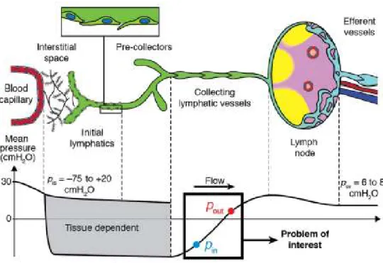
In this context, the target of our thesis is to develop two computational environments which enable us to study the fluid dynamic features of the lymphatic system as illustrated in Figure 1.1.
Figure 1.1: Conceptual structure of the problem of interest
To define the virtual laboratory, we consider an interdisciplinary approach involving both physiology and engineering.
In this chapter, we will provide an overview of the physiology of the lymphatic system, which is needed to define the theoretical basis of the problem as well as to elucidate challenges and open questions involved in its modeling.
Then, in Chapter 2, we will describe the mathematical framework of conservation laws of fluids on which our thesis is based. Specifically, we will describe two model reduction approaches of the latter equations which will provide two different perspectives of the problem at hand. In Chapters 3 and 4, we will consider a systemic perspective of the lymphatic at the scale of the human body employing a lumped parameter model based on fluid-electrical analogy. Based on the observations of this model, in Chapter 5 and 6, we will investigate the hydraulic behavior of a crucial component of the lymphatic physiology, called lymphangion, with a CFD approach. Finally, we will describe the conclusions and the perspectives of this
1.2 Lymphatic system
The lymphatic system is an organized network of several organs, tissues and vessels.
The lymphoid organs include the spleen, thymus and tonsils. Additional vital parts include the bone marrow, where white blood cells are produced, and lymph nodes, which are small bean-shaped glandular nodules where white blood cells can proliferate.
Figure 1.2: Lymphoid organs in the human body
The focus of this thesis is on the fluid-dynamic behavior of the lymphatic vascular system, which comprises a network of vessels extending to almost every organ, including the brain [4].
Lymphatic vessels carry lymph, which is a fluid containing mainly water, along with suspended proteins and immune cells. The anatomical region where lymph is formed is the intercellular space. Then, this network runs in parallel to the venous system and returns to the blood circulation through the thoracic ducts.
As can be observed in Figure 1.3, the cardiovascular system is a closed system where fluid leaves and returns from the same organ (the heart). Conversely, the lymphatic system begins at the interstitial space before returning to the blood circulation (it is called a blunt-ended linear system).
Figure 1.3: Schematic representation of the lymphatic system
1.2.1 Tasks of the lymphatic system
The lymphatic system was initially recognized solely as a network of transporting pathways for the removal of tissue products. After the discovery of the filtration process from the capillaries, the role of the lymphatic system in the maintenance of fluid-homeostasis by controlling extracellular fluid volume became more evident.
Specifically, the lymphatic system regulates both tissue fluid and transport of macromolecules, such as proteins, to blood, gathering them from the interstitial space and returning them to the blood system.
1.2.2 Lymphatic vascular system
The lymphatic transport system is composed of a hierarchy of vessels of increasing size which originates in the interstitial space with the initial lymphatic, or lymphatic capillaries, which are depicted in Figure 1.4.
Figure 1.4: Lymphatic capillaries
Lymphatic capillaries are supported by anchoring filaments and function as a one-way valve system to prevent back-flow. The small lymphatic capillaries gradually combine to form larger diameter vessels, called pre-collectors. They contain layers of smooth muscle and are capable of performing spontaneous contraction. Furthermore, pre-collectors have the task of collecting substances from the interstitial space and propelling them towards larger vessels, called the collecting lymphatic.
The structure of the collecting lymphatic is similar to that of blood vessel, and they contain another type of valve, called the secondary valve. The segment of the collecting lymphatics between valves is termed lymphangion and is represented in Figure 1.5.
The peculiarity of the latter element is that it can perform rhythmic contractions with which the lymph is propelled. Interestingly, the lymphatic transport system performs this pumping function in the absence of a central pulsatile organ.
1.2.3 Physiology of the lymphatic system
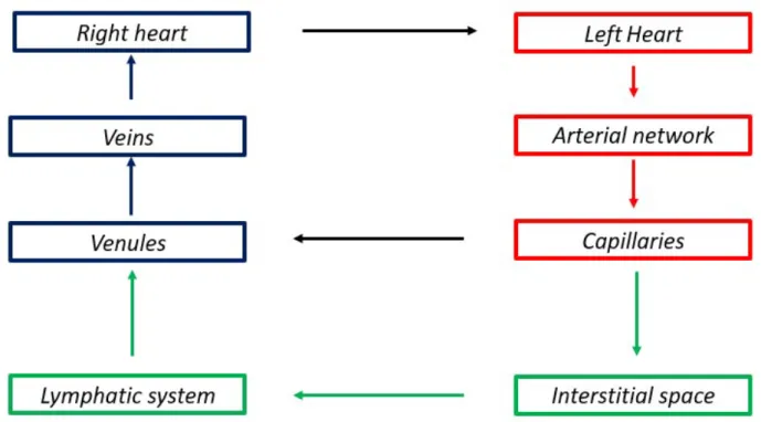
The lymphatic vascular system works in conjunction with the cardiovascular system and their relationship is schematically represented in Figure 1.6.
Figure 1.6: Relationship between the cardiovascular and the lymphatic system
As blood arrives at the capillary bed, it is forced out of the leaky barrier of these vessels.
Most of the exudate gets reabsorbed into the blood circulation, but there is an excess of fluid which filtrates into the interstitial space. For the maintenance of fluid homeostasis, this net flux must be acquired by the lymphatic system. Once the fluid enters the lymphatic system, it is propelled due to the rhythmic contraction of the lymphangions. The crucial importance of the contraction of lymphangions stems from the pressure boundary condition of the lymphatic flow pathways which can be observed in Figure 1.7.
Figure 1.7: Lymph flow pathway from the interstitial space to the subclavian vein
The interstitial space represents the inlet of this network of vessels and is characterized by a subatmospheric pressure. In contrast, the outlet point of lymphatic vasculature is the venular side where pressure is positive (6-8 mmHg). Hence, a propulsion is needed to allow fluid movement against a hydrostatic pressure gradient.
The driving force is provided by the rhythmic contraction of lymphangions, whose effectiveness impacts not only the interstitial fluid but overall homeostasis [4][7].
Despite the crucial importance of this process, the physiological mechanisms underlying the contraction rate are still not completely elucidated in the literature. Similarly, also the process with which we have an uptake of interstitial fluid has been subject of much controversy [10].
1.3 Lymphatic system in diseases
In this section we illustrate several disorders in which lymphatic system is involved.
1.3.1 Lymphedema
One consequence of inadequate lymph transport is lymphedema. This disease is a progressive pathological condition of the lymphatic system leading to the accumulation of a protein-rich interstitial fluid in the tissue. It is a debilitating disease which significantly affects the quality of life. Lymphedema usually involves swelling of a limb, but other areas, including the head, neck and breast may be involved. It can be distinguished into primary lymphedema and secondary lymphedema.
The first occurs in childhood and leads to alterations in the structural features of the lymphatic system while secondary lymphedema stems from a complication of cancer treatment or parasitic infections, but it can also be linked to several genetic disorders.
Specifically, in advanced countries, the majority of secondary lymphedema is observed among cancer patients who undergo various radiation therapies. Although it is an essential practice, it inevitably destroys and obstructs lymphatic flows and thus exposes patients to a high increased risk of lymphedema. Studies report that 25%–56% of breast cancer patients develop mild-to-severe lymphedema after cancer treatment [1].
Although lymphedema has been described for centuries, there is no cure for lymphedema. Successful management of the disease, resulting in its limiting progression, can be achieved with early diagnosis. The therapies for lymphedema include massage, bandages, and, in the most severe cases, the surgical removal of the tissue.
1.3.2 Metastases
All of the deadliest forms of cancer spread because metastatic cells separate from the primary tumor and migrate to different locations of the body through the cardiovascular or lymphatic system. The immune system is capable of eliminating these rogue cells. Unfortunately, this defense system can be overwhelmed or subverted, resulting in the formation of secondary tumors in other parts of the body. These secondary tumors that are actually responsible for approximately 90% of cancer deaths [11].
1.3.3 Immune system disfunction
Transport along the lymphatic flow delivers crucial information to lymph node.
Without the lymph flow–mediated transport of immune cells and antigens, there could be no adaptive immunity in animals. Moreover, the physiological mechanism of the lymphatic system, such as the contraction, may play an integral role in the immune system as described in [12].
GOVERNING EQUATIONS
The physical problem object of this thesis consists of investigating the fluid-dynamic behaviour in a biological system comprised of the lymphatic system in conjunction with the cardiovascular system within the human body. The biological system is schematically represented in Figure 2.1.
Figure 2.1: Cardiovascular and lymphatic system
In principle, to accomplish the target of this thesis we should study the following set of partial differential equations (PDEs).
𝛻 ⋅ 𝑣 = 0 Eq(2.1)
𝜕𝑣
𝜕𝑡 + 𝜌𝑣 ∙ 𝛻𝑣 + 𝛻𝑝 − 𝒅𝒊𝒗(𝜇𝑫(𝑣)) = 𝑓 Eq(2.2)
The Eq(2.1) is referred to as the mass conservation law and Eq(2.2) as the linear momentum balance law. The system of Eq(2.1) and Eq(2.2) is a closed set of equations whose unknowns are the three components of the fluid velocity 𝑣 and pressure p.
The solution of model Eq(2.1)-Eq(2.2) at the scale of the human body is unaffordable by a computational point of view. Hence, we will consider two model reduction approaches at two different scale to reduce the computational complexity of the problem.
2.1 Lumped parameter model
In this section, we define the governing equations of the lumped parameter model, which can be derived by general conservation principles. In section 2.1.1, we will initially describe the one dimensional (1D) conservation equation. Then, we derive the governing equations of the lumped parameter model and the fluid-electric analogy.
2.1.1 One-dimensional conservation equation
Figure 2.2 represents a simple compliant tube considered as a model of a human vessel. We assume that the axis of the vessel is rectilinear and coincides with the x-axis.
Figure 2.2 Compliant tube
𝜕(𝑓 𝐴) 𝜕𝑡 + 𝜕 𝜕𝑥 (𝑓𝑣 𝐴) = 𝜕𝑓 𝜕𝑡(𝑥, 𝑡) + 𝛻 ⋅ (𝑓𝑣) 𝑑𝜎 + 𝜌(𝑤 ∙ 𝑛)𝑑𝛾 Eq(2.3) where
- 𝑓 is the area-averaged value of f
𝑓 = 1
𝐴 𝑓 𝑑𝜎 Eq(2.4)
- A is the cross-section area
𝐴 = 𝐴(𝑥, 𝑡) = 𝑑𝜎
Eq(2.5)
- 𝑣
i
s the area-averaged value of the x-component of the velocity𝑣 = 1
𝐴 𝑣 𝑑𝜎 Eq(2.6)
If we assume that the lumen is impermeable, i.e. 𝑤 ∙ 𝑛 = 0 we get
𝜕(𝑓 𝐴) 𝜕𝑡 + 𝜕 𝜕𝑥 (𝑓𝑣 𝐴) = 𝜕𝑓 𝜕𝑡(𝑥, 𝑡) + 𝛻 ⋅ (𝑓𝑣) 𝑑𝜎 Eq(2.7)
One-dimensional conservation of mass is obtained considering by setting 𝑓 = 𝜌 in Eq(2.7), namely
𝜕(𝜌 𝐴) 𝜕𝑡 + 𝜕(𝜌𝑣 𝐴) 𝜕𝑥 − 𝜕𝜌 𝜕𝑡 𝑥, 𝑡 + 𝛻 ⋅ 𝜌𝑣 𝑑𝜎 = 0 Eq(2.8)
If we assume that the density is constant and that the fluid is incompressible, i.e. 𝛻 ⋅ 𝑣 = 0, we get
𝜕𝐴 𝜕𝑡 +
𝜕(𝑣 𝐴)
𝜕𝑥 = 0 Eq(2.9)
Similarly, one-dimensional momentum balance is obtained by setting 𝑓 = 𝜌𝑣 in Eq(2.7). The formal derivation is provided [13] [14] [15], here we report the result
𝜕(𝑣 𝐴) 𝜕𝑡 + 𝜕(𝑣 𝐴) 𝜕𝑥 = 𝐴 𝜌 𝜌𝑓 − 1 𝜌 𝜕𝑝 𝜕𝑥 + 𝑑 Eq(2.10) where
- 𝑓 𝑏represents the z-component of the external force;
- 𝑑 d1 is the x-component of d, where 𝒅 = 𝛻 ∙ 𝑫 and 𝑫 represents the deviatoric stress tensor. The system of the above one-dimensional equations can be rewritten as
⎩ ⎪ ⎨ ⎪ ⎧ 𝜕𝐴 𝜕𝑡 + 𝜕(𝑣 𝐴) 𝜕𝑥 = 0 𝜕(𝑣 𝐴) 𝜕𝑡 + 𝜕(𝑣 𝐴) 𝜕𝑥 = 𝐴 𝜌 𝜌𝑓 − 𝜕𝑝 𝜕𝑥 + 𝑑 = 0 Eq(2.11)
The unknowns in the system are p, A and 𝑣 . Their number exceeds the number of equations and a common way to close the system is to find a relationship between pressure and area of the vessels [15].
2.1.2 Zero-dimensional equation
The governing equations of a lumped parameter model can be derived by averaging the 1D models. We will firstly reformulate Eq(2.11) by adding some hypotheses and modifying the notation.
Specifically:
- we will assume that external forces are negligible (𝑓1𝑏
= 0 );
- area averaged velocity and pressure will be denoted as v and p respectively. Moreover, we define the mass flux across a section as
𝑄 = 𝑣 𝑑𝛺 = 𝐴𝑣 = 𝐴𝑣 Eq(2.12)
Introducing the above notation into Eq(2.11) yields:
⎩ ⎪ ⎨ ⎪ ⎧ 𝜕𝐴 𝜕𝑡+ 𝜕𝑄 𝜕𝑥 = 0 𝜕𝑄 𝜕𝑡 + 𝜕(𝑣 𝐴) 𝜕𝑥 + 𝐴 𝜌 𝜕𝑝 𝜕𝑥 + 𝑑 𝑄 𝐴= 0 Eq(2.13)
Considering the blood vessels represented in Figure 2.2, we define its length as 𝑙 = |𝑥 − 𝑥 |, we can define the mean volumetric flow rate over the whole vessel as
𝑄 =𝜌
𝑙 𝑣 𝑑𝑉 = 𝑣 𝑑𝑆 =
𝜌
𝑙 𝑄(𝑥) 𝑑𝑥 Eq (2.14)
Similarly, we define the mean pressure and area over the vessel as
𝑝̂ =1
Regarding the momentum equation, we add the following simplifying assumptions: the contribution of the convective term ( )can be neglected [13], [15];
the variation of A with respect to x is small compared to that of P and Q. We can replace A with a constant value for the area that in general is assumed to be the area at rest A0.
Averaging along x direction we get
𝑑𝑄 𝑑𝑡 + 𝑑 𝐴 𝑄 + 𝐴 𝜌 (𝑃 (𝑡) − 𝑃 (𝑡)) = 0 Eq (2.18) where 𝑃 (𝑡) = 𝑃 (𝑡 , 𝑥 ) = 0 Eq (2.19)
Hence, the zero-dimensional format of the mass and balance conservation reads as
⎩ ⎪ ⎨ ⎪ ⎧ 𝑙𝑑𝐴 𝑑𝑡 + 𝑄 (𝑡) − 𝑄 (𝑡) = 0 = 0 𝑑𝑄 𝑑𝑡 + 𝑑 𝐴 𝑄 + 𝐴 𝜌 (𝑃 (𝑡) − 𝑃 (𝑡)) = 0 Eq(2.20)
We again have again problem of closing the system by adding a wall mechanics law. For instance, we can consider the relation proposed by [15]
𝑑𝐴
𝑑𝑡
= 𝑘
𝑑𝑝̂
𝑑𝑡
Eq (2.21) where -
𝐾 =
-𝛽 =
( ) we get ⎩ ⎪ ⎨ ⎪ ⎧ 𝑙𝑘 𝑑𝑝̂ 𝑑𝑡 + 𝑄 (𝑡) − 𝑄 (𝑡) = 0 = 0 𝑑𝑄 𝑑𝑡 + 𝑑 𝐴 𝑄 + 𝐴 𝜌(𝑃 (𝑡) − 𝑃 (𝑡)) = 0 Eq(2.22)2.1.3 Fluid electric analogy
Equations such as Eq(2.22) are also found in the analysis of electrical circuits.
As a matter of fact, the fluid-dynamic behaviour of both cardiovascular system [16][22] and lymphatic system [18] has been studied relying on electric circuit analogs.
The advantage of this approach is that we can solve the fluid-dynamic behaviour of a hydraulic system exploiting Kirchhoff’s laws of voltage and currents leading to a system of ordinary differential equation
(ODEs). Specifically, in this analogy, the blood (or lymph) flow rate is assimilated to the current, while pressure corresponds to voltage.
Starting, from this analogy, we can rewrite Eq(2.22) as
⎩ ⎨ ⎧ 𝐶𝜕𝑝̂ 𝜕𝑡 + 𝑄 − 𝑄 = 0 𝐿𝜕𝑄 𝜕𝑡 + 𝑅𝑄 + 𝑃 − 𝑃 = 0 Eq(2.23)
where the coefficient R, L, C are associated to the following electric elements:
- C is the capacitance and it is associated with the capacitor represented in Figure 2.3
Figure 2.3: Capacitor
Specifically, based on fluid-electric analogy the capacitance C is defined as
𝐶 = 𝑘 𝑙
Eq (2.24)and represents the mass storage term in the mass conservation law due to the compliance of the vessel.
- R is the resistance as depicted in Figure 2.4
instance, if we assume Poiseuille flow and that the vessel is a cylinder of constant circular cross section we have
𝑅 =
8𝜋𝜌𝜈𝑙
𝜋 𝑟
Eq (2.26)- L is the inductance and it is associated to the inductor represented in Figure 2.3
Figure 2.5: Inductor It is defined as
𝐿 =
𝜌𝑙
𝐴
Eq (2.27)and represents the inertial term in the momentum equation.
2.2 THE CFD APPROACH
In section 2.1 we showed the lumped model parameter reduction. This approach has the advantage to provide a systemic discretization of the problem of interest. Another typology of model reduction is based on a CFD approach, where the target is a discretization of the equation system (2.1) – (2.2) at a local scale to investigate the fluid-dynamic behaviour of the problem at hand. Specifically, we will use a CFD commercial software, called FLOW-3D (described in Chapter 5), based on the finite volume that is described below.
We consider the balance law of the scalar quantity 𝑢 = 𝑢(𝑥, 𝑡)
𝜕𝑢
𝜕𝑡
+ 𝛻 ∙ 𝐹(𝑢) = 𝛽
Eq (2.28) The flux 𝐹accounts for two contributions𝐹(𝑢) = 𝐹
(𝑢) + 𝐹
(𝑢)
Eq (2.29)where
𝐹
(𝑢) = 𝑣 ∙ 𝑢
Eq (2.30)and
𝐹
(𝑢) = −𝐷 𝛻𝑢
Eq (2.31)The model Eq(2.29)- Eq(2.30)- Eq(2.31) is the scalar version of the flux in the momentum balance equation Eq(2.2) written in the conservative form. The function 𝛽 = 𝛽(𝑥, 𝑡) is the net production rate.
The balance law Eq(2.28), with the constitutive relations Eq(2.29)- Eq(2.30)- Eq(2.31), must be solved in a domain 𝛺 ⊆ ℝ , d =1,2,3, and in a time interval 𝐼 = (0, 𝑇) , 𝑇 > 0 supplied by initial and boundary condition.
To proceed with the finite volume method we assume that 𝛺 is a polygon in ℝ and we partition 𝛺 into a finite number of rectangular elements K
Figure 2.6: Computational domain Ω and partition 𝜁
We denote by
𝜁
the minor of the element K, ℎ > 0 being the discretization parameter. This latter is definedas the longer edge of 𝜁
Then we integrate the balance law Eq(2.28) over each element K
𝜕𝑢
𝜕𝑡𝑑𝐾 + 𝛻 ∙ 𝐹(𝑢) 𝑑𝐾 = 𝛽 𝑑𝐾 ∀𝐾 ∈ 𝜁 Eq (2.32)
This is the integral form of the balance law over the element K.
The second integral on the left-hand side of Eq(2.32) is treated using the divergence theorem to obtain:
𝜕𝑢
Figure 2.7:The element K and outward normal
The finite volume method is the numerical approximation of Eq(2.33) and is constructed by replacing 𝑢| with a constant 𝑢 the source term β with its value βKat the baricenter Ck and the normal component
of 𝐹 on each edge 𝑒 , 𝑖 = 1, . . ,4 with the constant fi where
𝑓 = 𝑓 (𝑢 , 𝑢 )
Eq (2.34)Ki being one of the four neighbouring element of K with respect to the edge 𝑒 .
The finite volume formulation leads to the following system of ordinary differential equation
𝑑
𝑢
ℎ𝑘𝑑𝑡 ∙ |𝑘| +
𝑓
𝑖(𝑢
ℎ𝑘, 𝑢
ℎ 𝑘𝑖)
∙ |𝑒 | = 𝛽 |𝑘| ∀𝐾 ∈ 𝜁 Eq (2.35)that has to be integrated on the time interval 𝐼 , given an initial datum 𝑢ℎ,0𝑘
,
∀𝐾 ∈ 𝜁 , the boundarycondition and a constitutive equation for fi.
System Eq(2.35) is the analog of the equation system of ODEs Eq(2.22) in the case of the model balance law.The approach discussed above is implemented in the package FLOW-3D and we refer to [Manuale FLOW-3D] for a documentation on the software.
We refer to [47] for a general description of the approximate normal component fi. and the analysis of the
A SYSTEMIC LUMPED PARAMETER MODEL
OF FLUID BALANCE IN THE HUMAN BODY
The aim of the first part of the thesis is to develop a numerical environment to study the role played by the lymphatic system in maintaining a homeostasis condition in the human body. To pursue this target, we will provide a systemic description of human fluid balance which will constitute the global framework to investigate the impact of the lymphatic system. Owing to the scale of the problem, the adopted formulation is a lumped parameter model of the cardiovascular and lymphatic system based upon the equivalence of fluid and electric variable described in Chapter 2.
Concerning the cardiovascular system, we will illustrate a possible electric description of the arterial and venous network and of the heart. Then, we will describe the numerical implementation of the proposed formulation of the cardiovascular system with two different software (MatLab and OpenModelica). Finally, we will introduce the electric counterpart of both filtration process and the interstitial space, which will enable us to characterize lymphatic system and study human fluid balance in Chapter 4.
3.1 Lumped parameter modeling of fluid balance in the
human body
In this chapter we illustrate the features of the computational environment to study the interaction between the lymphatic system and the cardiovascular system. These two systems work in conjunction to maintain a homeostasis condition in the global balance of fluid circulating in the human body and they are the key components of our model.
3.1.1 Structure of the model
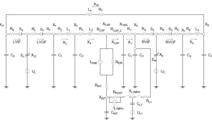
A lumped parameter model of a hydraulic system is based on the key concept of compartment, which is a spatially homogeneous unit function of the sole time variable and characterized by a pressure and a flow rate. The model proposed in the present thesis comprises eight connected compartments, as depicted in Figure 3.1. Specifically, the compartment of heart, arteries, veins and capillaries describe the cardiovascular system whereas the interstitial space and the lymphatic system define the systemic microcirculation. Overall, each compartment collaborates in maintaining human fluid balance.
Figure 3.1:Block diagram of the proposed model of human fluid balance
The hemodynamic features of each compartment in the scheme of Figure 3.1 can be described with a combination of electrical elements based on the fluid-electric equivalence already treated in Chapter 2. Moreover, the block diagram depicted in Figure 3.1 is the mathematical counterpart of the cardiovascular system and lymphatic system illustrated in Figure 3.2.
Figure 3.2:Cardiovascular and Lymphatic system
The objective of these chapters is the definition and the calibration of a proper representation of the physiology of each compartment to construct a model comprising of:
- Cardiovascular system;
- Filtration/reabsorption process taking place at the capillary side of systemic circulation; - Interstitial space.
This formulation will represent fluid balance in a healthy physiological condition.
In the next section we present a review of the lumped parameter modeling of the arterial and venous tree, that will be used to develop the global lumped model describing human fluid balance.
3.1.2 Single and multi-compartment models of arterial and
venous trees
The cardiovascular system has been the first element of human physiology studied with electric components since the 19th century. Frank Windkessel in 1899 formulated the first model, called 2 element
WK, to describe the hemodynamic property of arterial network [19]. The model comprises a resistor connected in parallel with a capacitor, as depicted in Figure 3.3. It accounted for the total resistance of the systemic vasculature and the elasticity of large arteries.
Figure 3.3: 2-element WK model
The 2 element WK is appropriate to describe aortic pressure decay in diastole, but it does not account properly for systole description [19]. Therefore, a characteristic impedance was introduced as an improvement of the classic two-element Windkessel formulation. This impedance has the same units as a resistor but has the role to describe wave traveling along the arterial system. The three-element Windkessel is represented in Figure 3.4.
Figure 3.4: 3-element WK model
Later, Stergiopulos added an inductive element introducing the 4-element WK model reported in Figure 3.5. This fourth element represents the total arterial blood inertia of the cardiovascular system and corrects low frequency behaviour where the 3-element WK model fails to be accurate [47].
distal vascular system”. To overcome this limitation, a multi-compartment model must be considered to partition the systemic circulation in several interacting units. This description enables us to calculate flow and pressure in different parts of the cardiovascular tree.
For instance, the arterial tree may be subdivided into large and small arteries. The first group includes the aorta, the main high-pressure pipeline connected to the heart left ventricle, and other main arteries such as the femoral and the brachial one. Large arteries are quite elastic vessels where blood flow is pulsatile. Thus, the full resistance, compliance, and inductance effects need to be considered [21]. The electric circuit describing these effects is reported in Figure 3.6 and is called RLC combination.
Figure 3.6:RLC combination
This circuit is mathematically described by:
𝑄 = 𝐶𝑑𝑃 𝑑𝑡 + 𝑄
𝑃 − 𝑅𝑄 − 𝑃 − 𝐿𝑑𝑄
𝑑𝑡 = 0
Eq(3.1)
This system of equation (3.1) is found applying Kirchhoff’s current law to node 1 and Kirchhoff’s voltage law to the closed loop between node 1 and 2. The RLC combination is adopted in [22] and in [24] to describe large arteries within a multi-compartment model.
Moreover, in [25] a comparison between a linear and nonlinear formulations of the compliant element is presented. The conclusion of this work is that “no additional information is gained when a pressure-dependent, rather than a constant, compliance throughout the heartbeat is incorporated in the three-element Windkessel. Nor does the nonlinear model significantly improves the three-three-element Windkessel”. In [21] the modeling choice of neglecting pressure dependency of large arteries is further justified by the fact that “the diameter changes in the arterial system are relatively small (order of 10%), and that the range of arterial pressures over the cardiac cycle is such that the material tends to operate in a relatively linear region of the stress-strain curve”. Accordingly, we can conclude that a RLC combination with constant parameters can be considered a proper representation of these vessels.
Concerning small arteries, they comprise a network of vessels that extend throughout the body. As done in [22], the RLC combination can be used to describe hemodynamic features of this latter compartment.
To complete the description of the arterial tree we need also to consider the arterioles. Those vessels have a relatively rigid wall, the flow is steady and frictional loss is the dominant factor, thus a pure resistance element adequately describes the local flow dynamics [16]. Furthermore, one peculiar property of arterioles is autoregulation, which is the ability to maintain a relatively constant level of blood flow despite changes in perfusion pressure. Autoregulation is achieved by varying the vascular tone of smooth muscles, causing the vessels to constrict or dilate to adjust themselves to a variation of pressure and flow rate. We must account for autoregulation in a pathological condition and, from an electric point of view, it will result in a non-linear relation of the resistance describing this compartment.
Regarding the venous tree, these vessels provide a reservoir function for storing large quantities of extra blood that can be called into use whenever required elsewhere in the circulation [26]
The peculiar feature of veins is their distensibility ([27] reported the central veins to be 8 times as distensible as central arteries) and accordingly, the venous system is usually represented with a compliance. For instance, Figure 3.7 shows the modelling choice done in [15], where the venous system is represented by the capacitor 𝐶 and it is included in a lumped parameter model of the whole cardiovascular tree.
Figure 3.7: Lumped parameter representation of the venous system
Flow in veins is also pulsatile but in a more regular way than in the arteries and usually inertial effects can be neglected. For instance, this is the modeling choice done in [22] and [27] where the venous system is described with a capacitance and a resistance. Moreover, according to [21] when veins enter a collapsed state, we should consider the pressure dependency of these vessels. As in the case of autoregulation for arterioles, this property must be accounted for to describe a pathological condition.
3.2 Lumped parameter description of the heart and its
contractile property
In this section we complete the overview of the cardiovascular circulation by illustrating the lumped parameter description of the heart. To pursue the target, initially we present a theoretical overview regarding the so-called PV loop, a physiological plot describing the contractile properties of ventricles, and the concept of elastance. Then, we will introduce the concept of time-varying elastance which provides a mathematical description of heart pumping function. Finally, we will illustrate the mathematical representation of this model proposed in [17].
3.2.1 Representation of the cardiac cycle through the PV loop
Cardiac cycle is the period required for one heartbeat. It is composed of a systole and of a diastole, which are the moments when heart contracts and relaxes causing its chambers to increase and decrease their stiffness, respectively. These two phases can be represented with the graph reported in Figure 3.8, called P-V loop (Pressure-Volume), which represents the instantaneous relationship between intraventricular pressure and volume through one cardiac cycle. Specifically, systole happens between point 1 and 4 whereas diastole between point 4 and 1.
Figure 3.8: Cardiac Pressure-Volume Loop
This graph has been widely used to analyse cardiac mechanics. Specifically, contractile properties of ventricles can be represented with two pressure-volume curves in the P-V plane. The first one is the end-diastolic pressure-volume relationship (EDPVR), reported in Figure 3.9. This curve describes the passive filling of the ventricle and thus the passive properties of the myocardium.
Figure 3.9: Graphical representation of the EDPVR
Quantitative analysis of the EDPVR curves has shown that pressure and volume are related by a nonlinear function, namely
𝐸𝐷𝑃𝑉𝑅 = 𝑃 + 𝛽𝑉 Eq(3.2)
where V is the volume inside the ventricle, 𝑃 is the pressure asymptote at low volumes and α and β are constants specifying the curvature of the line depending on properties of the ventricle. The slope of the EDPVR at any point along this curve is the reciprocal of ventricular compliance and is called elastance. By a dimensional point of view, it is defined as
𝐸(𝑡) =[𝑉] [𝑃]=
[𝐿 ]
[𝑀] ∙ [𝐿 ] ∙ [𝑇 ] Eq(3.3)
At the opposite extreme of the cardiac cycle, when muscles are in their maximally activated state, we can define the second pressure volume relationship curve, called end-systolic pressure volume relationship (ESPVR). This curve describes the maximal pressure that can be developed at any given ventricular volume and is expressed by a linear relationship, namely
𝐸𝑆𝑃𝑉𝑅 = 𝑃
𝑉 − 𝑉 Eq(3.4)
where Pes is the end-systolic pressure, Vo is a slightly positive volume remaining in the heart chamber at the end of the contraction and V is the volume. The slope of the ESPVR represents the end-systolic elastance, which provides an index of myocardial contractility and it can be considered an improved index of systolic function. These ESPVR and EDPVR are reported in Figure 3.10.
Figure 3.10: ESPVR and EDPVR in the PV plane
We can notice how the PV loop cannot cross over the line defining ESPVR for any given contractile state whereas EDPVR provides a boundary on which the PV loop falls at the end of the cardiac cycle.
Starting from these concepts we can describe the theory of the time-varying elastance.
3.2.2 Theory of time-varying elastance
The time-varying elastance model stems from the work performed by Suga and Sagawa in the early 1970s [28]. Starting from in-vivo experiments on an isolated canine left ventricle, these two authors analysed cardiac mechanics in the pressure-volume plane. Their experimental data reported in Figure 3.11 suggest how the left ventricle can be considered as a 2-state device.
Figure 3.11: Time-varying elastance concept from [28]
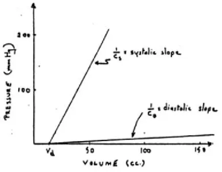
As a matter of fact, in the diastole the heart behaves as an elastic chamber whose properties may be represented by a diastolic pressure-volume linear curve
𝑉 = 𝑉 + 𝐶 ∙ 𝑃
Eq(3.5)
Similarly, during systole, the heart can be represented as a capacitor characterized by another linear pressure volume relation
𝑉 = 𝑉 + 𝐶 ∙ 𝑃 Eq(3.6)
These relations are plotted below in the pressure-volume plane in Figure 3.12.
Figure 3.12: ESPVR and EDPVR in the time-varying elastance model
The previous analysis led to the definition of the time-varying elastance model [28], which relates the left-ventricular pressure P(t) and volume V(t) according to the following linear relationship:
𝐸(𝑡) = 𝑃 (𝑡)
𝑉 (𝑡) − 𝑉 Eq(3.7)
with E = elastance, a time-dependent slope, and V0, the fixed volume-axis intercept.
Since Eq (3.7) describes a linear dependence between pressure and volume, each time instant of the cardiac cycle in the PV loop can be described by a (generally different) value of the elastance. This concept is illustrated in Figure 3.13. Specifically, the time rate of change of elastance in the PV loop during systole and diastole is represented in the left and right panel, respectively.
Figure 3.13: Time rate of change of elastance in the PV plane during systole and diastole
If we plot each value of the elastance as a function of time, we can observe a smooth transition during the cardiac cycle represented by the sinusoidal function depicted in Figure 3.14, called activation function.
Figure 3.14:Activation function of the time-varying elastance
This function represents the time-varying elastance and it can be adopted to reproduce heart contractility. The peculiar properties of this model are that in the left ventricle the elastance function is independent of the load against which the ventricle ejects [28] and that this description included the effect of ventricular filling on ventricular contraction [29].As such, being independent of afterload and inherently containing the effect of preload, the time-varying elastance model can be considered as a constitutive equation for the ventricle that linearly relates ventricular volume to intracavity pressure according to Eq (3.7). Afterwards, it was demonstrated that, after normalizing the time-varying elastance curve, the shape was constant within one species and in a large range of cardiac diseases and it exhibited a smooth transition between ESPVR and EDPVR which is reported in Figure 3.15.
Figure 3.15:Normalized elastance
There are two implications of the described model:
- if one knows the function E(t) and the time course of volume changes during the cycle, it is possible to predict the time course of pressure changes throughout the cycle;
- Since the elastance is the inverse of a compliance, this model has been widely used to represent with a lumped approach the mechanical property of the heart as shown in the next section.
3.2.3 Lumped parameter description of the heart
One of the first lumped parameter model of the heart was developed by [30]. He represented the ventricle “as a two-component pressure source comprising an active contractile element and a series elastic element”.
After the appearance of the time-varying elastance model, several lumped formulation of the heart have been based on that concept. For instance, in [20] the heart contractile properties are described with a capacitor based on the observations of Suga et Al. We report in Figure 3.17 the representation of the left ventricle.
Figure 3.17:Lumped modeling of the left ventricle [from 31]
Specifically, the instantaneous volume change in the left ventricle is equal to the flow rate difference:
𝑑𝑉
𝑑𝑥 = 𝑄 − 𝑄 Eq(3.8)
and the pressure is computed
𝑃 = 𝑃 , + 𝐸(𝑡) ∙ (𝑉 − 𝑉 ) Eq(3.9)
where the elastance is defined as:
𝐸(𝑡) = 𝐸 , +
𝐸 , − 𝐸 ,
2 ∙ 𝑒̅ (𝑡)
Eq(3.10)
𝐸
, is the slope of the ESPVR described before and𝐸
, is the slope of the linearized EDPVR while𝑒̅
is the so-called activation function, which describes the contraction and the relaxation changes in the ventricular volume, and it is defined as:
𝑒̅ = ⎩ ⎪ ⎪ ⎨ ⎪ ⎪ ⎧ 1 − 𝑐𝑜𝑠 𝑡 𝑇 𝜋 0 ≤ 𝑡 ≤ 𝑇 Eq(3.11) 1 + 𝑐𝑜𝑠 𝑡 − 𝑇 𝑇 − 𝑇 𝜋 𝑇 ≤ 𝑡 ≤ 𝑇 0 𝑇 ≤ 𝑡 ≤ 𝑇 where:
Ts1= time corresponding to the peak of systolic phase; Ts2=time corresponding to the end of systolic phase; T=heart period.
In the model it is also considered the possibility for the atrium to contract. Similarly with the ventricle, the atrium is modeled introducing the following variable elastance:
𝑒 (𝑡) = 𝐸 , +
𝐸 , − 𝐸 ,
2 ∙ 𝑒̅ (𝑡) Eq(3.12)
In which the atrium activation function is defined as
𝑒̅ = ⎩ ⎪ ⎪ ⎨ ⎪ ⎪ ⎧ 0 0 ≤ 𝑡 ≤ 𝑇 Eq(3.13) 1 − 𝑐𝑜𝑠(𝑡 − 𝑇 𝑇 2𝜋) 𝑇 ≤ 𝑡 ≤ 𝑇 + 𝑇 0 𝑇 ≤ 𝑡 ≤ 𝑇
In Figure 3.18 we report both the ventricular and atrium time-rate of change of elastances.
Figure 3.18: time-rate of change of elastances in the atrium and in the left ventricle [from 31]
Heart properties are described using the concept of time-varying elastance also in [22] and [16]. All these models are based on the observation of Suga et al but they are characterized by different assumptions in the derivation of the activation function.
Another possible lumped representation of the heart is described in Quarteroni [15], where a non-linear model is proposed as follows. As a first step, the authors introduce a relation linking internal pressure with the radius of an elastic spheric ball filled with fluid, namely
𝑃 =
2𝐸(𝑡)ℎ
3𝑅
3
4𝜋
/𝑉
/∙ (𝑉 − 𝑉 )
Eq(3.15)Introducing the capacitance C(t)
𝐶(𝑡) =
3𝑅 𝑉
/2𝐸(𝑡)ℎ
4𝜋
3
/ Eq(3.16)we can rewrite Eq (3.16) as follow
𝑉(𝑡) = 𝐶(𝑡) ∙ 𝑃(𝑡) + 𝑉 (𝑡)
Eq(3.17) Differentiating with respect to time yields𝑑𝑉
𝑑𝑡
= 𝑄 =
𝑑𝐶
𝑑𝑡
𝑃 + 𝐶
𝑑𝑃
𝑑𝑡
+ 𝑀 (𝑡)
Eq(3.18)Whose electric representation is reported in Figure 3.19
Figure 3.19: Electrical representation of heart model described in [15]
In Figure 3.19, the diodes are the electrical equivalent of valves and the resistance R accounts for additional resistance inside the ventricle. Throughout all the above described lumped descriptions of the heart, we consider in this thesis the model embedding the concept of time-varying elastance because of its physiological property described in Section 3.2.1. Specifically, we adopt the model of Avanzolini [17], [22] because of the detailed derivation of the time-varying elastance based on physiological concepts. In the next section we will describe its numerical derivation.
3.2.4 Mathematical description of the time-varying elastance
Avanzolini used the concept of time-varying elastance to describe an electrical analog for the two heart chambers based on a linearization of the pressure-flow relationship. The model is based on the following assumptions:
- the cardiac wall is a homogeneous medium with isotropic properties; - thick-walled spherical geometry;
- passive pressure depends exclusively on ventricular volume;
- active pressure (tightly related to pumping functions) depends on the ventricular volume V and the rate of volume change 𝑉̇;
Starting from these assumptions, the objective is the definition of a suitable linear approximation of the active pressure
𝑃
with respect to V and𝑉̇,
namely𝑃 (𝑡, 𝑉, 𝑉̇) = 𝑃 − 𝑃 = 𝑎(𝑡) ∙ 𝑃 (𝑉 ) + 𝑎(𝑡) ∙ 𝐾 ∙ (𝑉−𝑉 ) + 𝑎(𝑡) ∙ 𝑅 ∙ 𝑉̇ Eq(3.19)
where:
-
𝑃
represents the pressure developed inside the ventricle chamber; -𝑃
represents the passive pressure;-
𝑎(𝑡)
is the activation function;-
𝑃
is the isometric peak active pressure related to the Frank-Starling mechanism; -𝑉
is the volume corresponding to𝑃 ;
- K and R have the units of a stiffness and viscosity, respectively.
From a physical point of view
𝑎(𝑡) ∙ 𝑃 (𝑉 )
is the isovolumically developed active pressure while𝑉̇
is the rate of volume change representing the difference between atrial and aortic flow.This
pressure description can be represented by the electrical analog circuit depicted in Figure 3.21- a resistive element 𝑎(𝑡) ∙ 𝑅 across which a pressure drop proportional to flow is developed; - a capacitive element whose stiffness is 𝑎(𝑡) ∙ 𝐾.
Both viscosity and stiffness vary with time in linear proportion to activation a(t), whereas R and K can be obtained through a calibration procedure. The similarity with the description of Suga, where the isovolumic pressure and the stiffness were combined to a single elastic element, can be observed defining
𝐸(𝑡) = 𝑎(𝑡) ∙ 𝐾 Eq(3.20)
and
𝑉 = 𝑉 −𝑃
𝐾 Eq(3.21)
By doing this, the model can be expressed as:
𝑃 (𝑡, 𝑉, 𝑉̇ ) = 𝐸(𝑡) ∙ (𝑉−𝑉 ) + 𝑎(𝑡) ∙ 𝑅 ∙ 𝑉̇ Eq(3.22)
Eq(3.22) represents a classic time varying elastance model (the first-term on the right-hand side) with the addition of a time-viscous element (the second term on the right-hand side).
Finally, the ventricular pressure is given by:
𝑃 =
𝑈 + 𝐸 (𝑉 − 𝑉 ) + 𝑅 𝑉̇ 𝑠𝑦𝑠𝑡𝑜𝑙𝑒
Eq (3.23)
𝐸 (𝑉 − 𝑉 ) 𝑑𝑖𝑎𝑠𝑡𝑜𝑙𝑒
where:
-
𝑉
is the reference volume;
-𝑈 = 𝑎(𝑡) ∙ 𝑃 (𝑉 );
-
𝐸 = 𝐸 + 𝐸 .
The activation function is described by the following sinusoidal function
𝑎(𝑡) = 1 − 𝑐𝑜𝑠 2𝜋𝑡 𝑡 /2 0 𝑠𝑦𝑠𝑡𝑜𝑙𝑒 𝑑𝑖𝑎𝑠𝑡𝑜𝑙𝑒 Eq (3.24)
This model reproduces the effect of an increased in the volume of blood in the ventricle while the atrial pumping function are neglected. Moreover, based on the good fit with experimental data of this model, in [17] it is stated that “..interpretation of the success of this model is that the difference between isovolumic left ventricular pressure and pressure developed during an ejecting beat is accounted for by viscosity and stiffness, each of which varies with time in linear proportion to activation”.
In a subsequent paper, the author embeds this model into a more general one representing a systemic description of the cardiovascular apparatus [22]. The more general formulation model will represent the foundation of the model proposed in this thesis.
3.3 Lumped parameter model of the cardiovascular
system in a physiological healthy situation
In this section we will implement the computational model of the cardiovascular system. Initially, we will summarize the features of the reference model proposed in [22]. Then, we will modify this formulation to account for the filtration process, which will play a crucial role later in this thesis.
Finally, in section 3.3.3 we will implement the novel electrical circuit in both Matlab and OpenModelica computing environment.
3.3.1 Description and development of Avanzolini’s model
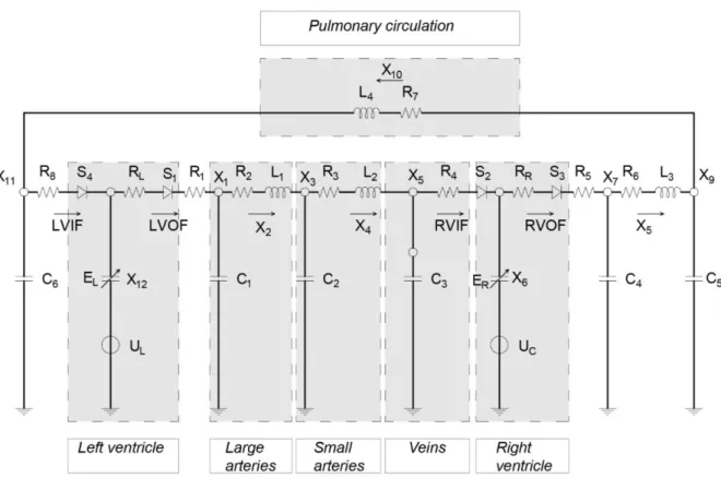
We consider Avanzolini’s model [22] as the starting point for the definition of the lumped model of the cardiovascular system. It is a multi-compartment model based upon fluid-electric analogy. The model is able to reproduce the main features of the cardiovascular system and consists of a closed loop.
The model is depicted in Figure 3.21.
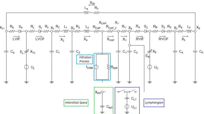
Figure 3.21: Lumped parameter model of the cardiovascular system
In the electrical circuit each node represents the pressure typical of a human compartment. We can match each electrical nodes with the corresponding physiological counterpart by comparing the pressure magnitude of each unit. For instance, we report below the range of the pressure in three nodes of the circuit
Node number Range of pressure Physiological compartments
X1 80-120 mmHg AORTA
X3 75-105 mmHg SMALL ARTERIES
X5 6-3 mmHg VEINS
Table 3.1 :Pressure in arterial and venous trees from [22]
With a similar procedure, we describe the physiological compartments described in the model: - large and small arteries, which are both described through a RLC combination; - veins, modeled with a capacitor and a resistor;
- the heart is represented with the diodes, representing the valves, combined with a capacitor and a potential source embedding time-varying elastance model;
- Pulmonary circulation. which is described through an inductor and a resistor
These physiological compartments are highlighted in Figure 3.22.
Figure 3.22: Physiological compartments described in the model of the cardiovascular system
Starting from the reference model of Avanzolini, we must address some issues to obtain a well-suited computational environment for our purposes. A first point is related to the level of physiological detail of the electrical circuit represented in Figure 3.22. As described in Section 3.1.1, we must reproduce process