UNIVERSITY
OF TRENTO
DEPARTMENT OF INFORMATION AND COMMUNICATION TECHNOLOGY
38050 Povo – Trento (Italy), Via Sommarive 14
http://www.dit.unitn.it
SEMANTIC MATCHING
Fausto Giunchiglia and Pavel Shvaiko
April 2003
Technical Report # DIT-03-013
Also: In The Knowledge Engineering Review journal, 18(3):265-280,
2004.
Semantic Matching
Fausto Giunchiglia1, and Pavel Shvaiko1
1 DIT – Dept. of Information and Communication Technology,
University of Trento, 38050 Povo, Trento, Italy {fausto, pavel}@dit.unitn.it
Abstract
We think of match as an operator that takes two graph-like structures (e.g., database schemas or on-tologies) and produces a mapping between elements of the two graphs that correspond semantically to each other. The goal of this paper is to propose a new approach to matching, called semantic match-ing. As its name indicates, in semantic matching the key intuition is to exploit the model-theoretic information, which is codified in the nodes and the structure of graphs. The contributions of this paper are (i) a rational reconstruction of the major matching problems and their articulation in terms of the more generic problem of matching graphs; (ii) the identification of semantic matching as a new ap-proach for performing generic matching; and (iii) a proposal of implementing semantic matching by testing propositional satisfiability.
1 Introduction
The progress of information and communication technologies has made accessible a large amount of information stored in different application-specific databases and web sites. The number of different information resources is rapidly increasing, and the problem of seman-tic heterogeneity is becoming more and more severe, see for instance [12], [20], [10], [11], [3]. One proposed solution is matching. Match is an operator that takes two graph-like structures (e.g., database schemas or ontologies) and produces a mapping between elements of the two graphs that correspond semantically to each other. So far, with the noticeable exception of [19], the key intuition underlying all the approaches to matching has been to map labels (of nodes) and to look for similarity (between labels) using syntax driven tech-niques and syntactic similarity measures; see for instance [9], [14]. Thus for example, some of the most used techniques look for common substrings (e.g., ″phone″ and ″telephone″) or for strings with similar soundex (e.g., ″4U″ and ″for you″) or expand abbreviations (e.g., ″P.O″ and ″Post Office″). We say that all these approaches are different variations of
syn-tactic matching. In synsyn-tactic matching semantics are not analyzed directly, but semantic
correspondences are searched for only on the basis of syntactic features.
In this paper we propose a novel approach, called semantic matching, with the following main features:
• We search for semantic correspondences by mapping meanings (concepts), and not labels, as in syntactic matching. As the rest of the paper makes clearer, when mapping concepts, it is not sufficient to consider the meanings of labels of the nodes, but also the positions that the nodes have in the graph.
• We use semantic similarity relations between elements (concepts) instead of syntactic similarity relations. In particular, we consider relations, which relate the extensions of the concepts under consideration (for instance, more/less general relations).
The contributions of this paper are (i) a rational reconstruction of the major matching prob-lems and their articulation in terms of the more generic problem of matching graphs; (ii) the identification of semantic matching as a new approach for performing generic match-ing; and (iii) a proposal of using a decider for propositional satisfiability (SAT) as a possi-ble way of implementing semantic matching. The algorithm proposed works only on Di-rected Acyclic Graphs (DAG’s) and is-a links. It is important to notice that SAT deciders are correct and complete decision procedures for propositional logics. Using SAT allows us to find only and all possible mappings between elements. This is another major advantage over syntactic matching approaches, which are based on heuristics. The SAT-based algo-rithm discussed in this paper is a minor modification/extension of the work described in [19].
The rest of the paper is organized as follows. Section 2 introduces some well-known matching problems and shows how they can be stated in terms of the generic problem of matching graphs. Section 3 defines the notion of matching and discusses the essence of semantic matching. Section 4 provides guidelines to the implementation of semantic match-ing. Section 5 overviews the related work. Section 6 reports some conclusions.
2
Matching Problems
Major data and conceptual models representing information sources across the WWW are database schemas, XML schemas, and ontologies. Let us discuss them in detail.
2.1 Relational DB schemas
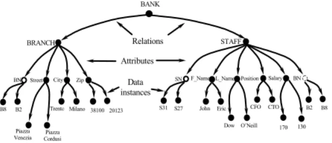
Let us consider the hypothetical relational database (RDB) BANK presented in Figure 1, storing information about the location of branches and of the staff that works at the BANK. BRANCH
BN Street City Zip
B8 Piazza Venezia Trento 38100
B2 Piazza Cordusio Milano 20123
STAFF
SN F_Name L_Name Position Salary BN
S31 John Dow CFO 170 B2
S27 Eric O’Neill CTO 130 B8
We can represent the schema and data instances of the above database as a graph in two possible ways. In the first case, starting from the name (root), the schema is partitioned into relations and further down into attributes and data instances. See Figure 2. Arcs of Level 1 encode relations; arcs of Level 2 stand for attributes, and arcs of Level 3 specify data in-stances. Blank nodes stand for primary keys. Blank nodes with dashed circles stand for foreign keys. Notice that we know in advance that the maximum height of the tree is 3.
Fig. 2. Tree representation 1 of the RDB BANK
In the second approach, as from [5], starting from the root, a database is partitioned into relations, then into tuples, and finally into attributes and data instances. See Figure 3. For lack of space not all attributes and their identifiers are presented in the diagram. Notice that the maximum height of the tree is 4.
The information about the structure of the database resides only at arcs’ labels. Dashed arcs stand for primary keys. R1 and R2 denote relations of the database BANK. ROOT.RI.TJ.AK is a path to the K-th attribute of the J-th tuple of the I-th relation from the root of the tree. Data instances are presented as arcs at Level 4. Thus, the instances of the element BRANCH are represented by tuples: (″B8″, ″Piazza Venezia″, ″Trento″, ″38100″) and (″B2″, ″Piazza Cordusio″, ″Milano″, ″20123″).
Fig. 3. Tree representation 2 of the RDB BANK STAFF R2 Tuple Tuple R2.T1 R2.T2 BRANCH R1 R1.T1 R1.T2 Tuple Tuple
BN City Street Zip BNCity Street Zip
B8 Piazza Venezia Trento 38100 B2 Piazza Cordusi Milano 20123 R1.T1.A1 ROOT B2 BRANCH STAFF BANK Zip BN Street City B8 Trento Milano 3810020123 Piazza
Venezia Cordusi Piazza
B2 CFO 170 S31 John Dow O’Neill CTO B8 130 S27 Eric
SN F_Name L_Name Position Salary BN
Relations Attributes
Data instances
Which of the two representations is more preferable depends on the concrete task, but its worth to note that it is always possible to transform one model into another.
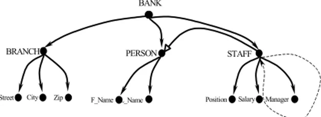
Database schemas are seldom trees. If referential constraints are taken into account, sche-mas become DAGs. If we further consider recursive references we have cycles, see for example Figure 4. Referential constraints are shown as dashed arrows. Bold arrows repre-sent recursive references, which appear if, for instance, we add to the relation STAFF the attribute Manager that expresses administrative relationships between employees.
Fig. 4. Graph representation of the RDB BANK
2.2 OODB schemas
Let us rebuild the relational database BANK example in terms of an object-oriented ap-proach. Now, BANK consists of the three classes, expressing the same data as above:
BRANCH(Street, City, Zip) PERSON(F_Name, L_Name)
STAFF:PERSON(Position, Salary, Manager).
A graph representation of the given OODB schema is shown in Figure 5. Arcs with blank arrows stand for the use case generalization; dashed arrows play notationally the same role as associations in UML.
Fig. 5. Digraph representation of the OODB BANK
The object-oriented data model captures more semantics than the relational data model. It explicitly expresses subsumption relations between elements, and admits special types of arcs for part/whole relationships in terms of aggregation and composition.
STAFF L_Name F_Name Zip City Street BRANCH PERSON BANK Manager Position Salary Zip BN Street City BRANCH B2 B8 Trento Milano Piazza
Venezia Cordusi Piazza 38100 20123
Position Salary BN STAFF Manager BANK SN F_Name L_Name Null S31 B2 CFO 170 S31 John Dow O’Neill CTO B8 130 S27 Eric
2.3 XML schemas
Neither the OO data model, nor the relational data model captures all the features of semis-tructured or unssemis-tructured data [6]. Semissemis-tructured data do not possess regular structure; the structure could be partial or even implicit. Missing or duplicated fields are allowed. Semis-tructured data could be schemaless, or have a schema that poses only loose constraints on data. Typical examples are markup languages, e.g., HTML or XML.
XML schemas can be represented as DAGs. The graph in Figure 2 could also be obtained from an XML schema. Often, XML schemas represent hierarchical data models. In this case the only relationships between the elements are {is-a}. A DAG is obtained through the ID/IDREF mechanism. Attributes in XML are used to represent extra information about data. There are no strict rules telling us when data should be represented as elements, or as attributes.
2.4 Concept Hierarchies
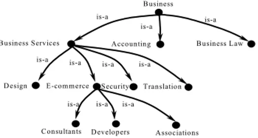
A concept hierarchy is a way of defining a conceptualization of an application domain in terms of concepts and relationships expressed in a formal language. Concept hierarchies usually support {is-a} relations. Traditional examples of concept hierarchies are classifica-tions, for instance, Yahoo and Google electronic catalogs. Figure 6 presents a part of Google web directory devoted to business.
Fig. 6. Google web directory
The concept hierarchy shown in Figure 6 consists of 11 concepts, and 10 subsumption relations, one per arc.
2.5 Ontologies
By an ontology we mean here a way of defining a conceptualization of an application do-main in terms of concepts, attributes, and relations expressed in a formal language. Rela-tions can be defined by the user, but there are some pre-defined relaRela-tionships with known semantics, i.e., {is-a; part-of; instance-of}. A concept hierarchy is an ontology without attributes and only with {is-a} relations between elements.
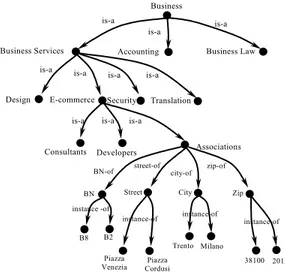
One example of ontology can be constructed by complicating the concept hierarchy shown in Figure 6, by adding attributes to the concept Association, see Figure 7. Attributes of the concept Associations are BN, City, Street, Zip, while data instances are B8 and B2. Data
Associations is-a is-a is-a is-a is-a is-a is-a is-a is-a is-a Security E-commerce Business Services B usiness Business Law Translation D esign Accounting Consultants D evelopers
instances have fixed attributes values: instance B8 has BN=″B8″, City=″Trento″, Street=″Piazza Venezia″, etc.
Fig. 7. Example of ontology Business
3 Matching
All the data and conceptual models discussed in the previous section can be represented as graphs. Therefore, the problem of matching heterogeneous and autonomous information resources can be decomposed in two steps:
1. extract graphs from the data or conceptual models, 2. match the resulting graphs.
Notice that this allows for the statement and solution of a more generic matching problem, very much along the lines of what done in Cupid [14], and COMA [9]. However, as al-ready discussed in some detail in Section 2, each of the five matching problems presented there, has different properties and it is still an open problem whether we will be able to develop a general purpose matcher, and exploit most (all?) the problem and domain de-pendent analysis in step (1).
Let us define the notion of matching graphs more precisely. Mapping element is a 4-tuple <
mID, Ni1, Nj2, R >, i=1...h; j=1..k; where mID is a unique identifier of the given mapping
element; Ni
1 is the i-th node of the first graph, h is the number of nodes in the first graph;
Nj
2 is the j-th node of the second graph, k is the number of nodes in the second graph; and R
specifies a similarity relation of the given nodes. A Mapping is a set of mapping elements.
Matching is the process of discovering mappings between two graphs through the
applica-tion of a matching algorithm. There exist two approaches to graph matching, namely exact
matching and inexact or approximate matching, see for instance [21]. Both of them can be
Associations is-a is-a is-a is-a is-a is-a is-a is-a is-a is-a Security E-commerce Business Services Business Business Law Translation Design Accounting Consultants Developers instance -of B2 B8 BN BN-of instance-of instance-of instance-of zip-of city-of street-of Zip City Street Trento Milano Piazza
stated as subgraph matching problems: find all occurrences of a pattern graph P of m nodes as a subgraph of a graph G of n nodes, m≤ n. In the case of exact matching we look for subgraphs S of G that are identical to P. In inexact matching some errors are acceptable. For obvious reasons we are interested in inexact matching.
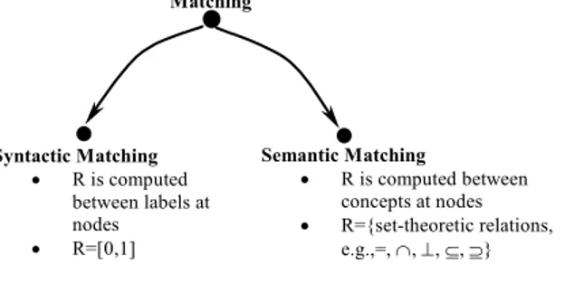
We classify matching into syntactic and semantic matching depending on how matching elements are computed and on the kind of similarity relation R used.
• In syntactic matching the key intuition is to map labels (of nodes) and to look for the similarity using syntax driven techniques and syntactic similarity measures. Thus, in the
case of syntactic matching, mapping elements are computed as 4-tuples < mID, Li1, Lj2, R
>, where Li
1 is the label at the i-th node of the first graph; Lj2 is the label at the j-th node
of the second graph; and R specifies a similarity relation in the form of a coefficient, which measures the similarity between the labels of the given nodes. Typical examples of R are coefficients in [0,1], for instance, similarity coefficients [14]. Similarity coeffi-cients usually measure the closeness between the two elements linguistically and struc-turally. For instance, based on linguistic analysis, the similarity coefficient between elements "telephone" and "phone" from the two hypothetical schemas could be 0,7. • As from its name, in semantic matching the key intuition is to map meanings
(con-cepts). Thus, in the case of semantic matching, mapping elements are computed as
4-tuples < mID, Ci1, Cj2, R >, where Ci1 is the concept of the i-th node of the first graph; Cj2
is the concept of the j-th node of the second graph; and R specifies a similarity relation in the form of a semantic relation between the extensions of concepts at the given nodes. Possible R’s between nodes are equality (=), overlapping (∩), mismatch (⊥), or more
general/specific (⊆, ⊇).
Fig. 8. Matching problems
Semantic Matching • R is computed between concepts at nodes • R={set-theoretic relations, e.g.,=, ∩, ⊥, ⊆, ⊇} Matching Syntactic Matching • R is computed between labels at nodes • R=[0,1]
These ideas are schematically represented in Figure 8. It is important to notice that all past approaches to matching we are aware of, with the exception of [19], perform syntactic matching.
One of the key differences between syntactic and semantic matching is that in syntactic matching, when we match two nodes, the meaning that we (implicitly) attach to them de-pends only on their labels, independently of their position in the graph. In semantic match-ing, instead, when we match two nodes, the concepts we analyse depend not only on the concept attached to the node (the concept denoted by the label of the node), but also on the position of the node in the graph. Let us consider the example in Figure 9. Numbers in circles are the unique identifiers of the nodes under consideration. A stands for the label at
a node; CA stands for the concept denoted by A; Ci stands for the concept at the node i (in
the following we sometimes confuse concepts with their extensions).
Fig. 9. Syntactic vs. semantic matching
Let us consider for instance, the analysis carried out when the node numbered 5 is submit-ted to matching (against a node in another graph). In syntactic matching the matcher tries to match the label at node 5, namely C. In semantic matching, instead, the matcher tries to
match the concept at node 5, namely C5, which is that subset of the extension of CA that is
also in the extension of CC. Thus, C5 = CA∩ CC. A semantic matcher will therefore try to
match CA∩ CC and not (!) C.
Let us consider some more examples, which make the consequences of the observation described in the previous paragraph clearer. For any example we also report the results produced by the state of the art matcher, Cupid [14], which exploits very sophisticated syntactic matching techniques. Notationally, in order to keep track of the graph we refer to we index nodes, labels, concepts and their extensions with the graph number (which is “1”
for the graph on the left and “2” for the graph on the right). Thus we have, for instance, A1,
51, CA1,C51.
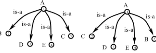
Analysis of siblings. Let us consider Figure 10. Structurally the graphs shown in Figure 10
differ in the order of siblings. Suppose that we want to match node 51 with node 22.
Fig. 10. Analysis of siblings. Case 1 A C B is-a is-a is-a is-a E D 1 4 3 5 2 A B C is-a is-a is-a is-a E D 1 4 3 5 2 A C B is-a is-a is-a is-a E D 1 4 3 5 2
Cupid correctly processes this situation, and as a result, the similarity coefficient between
labels at the given nodes equals to 0,8. This is because A1=A2, C1=C2 and we have the same
structures on both sides.A semantic matching approach compares concepts CA1 ∩ CC1 with
CA1 ∩ CC1andproduces C51 = C22.
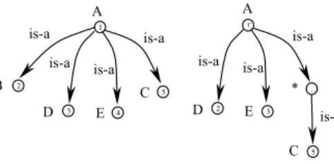
Analysis of ancestors. Let us consider Figure 11. Suppose that we want to match nodes 51
and 12.
Fig. 11. Analysis of ancestors. Case 1
Cupid does not find a similarity coefficient between the nodes under consideration, due to the significant differences in structure of the given graphs. In semantic matching, the
con-cept denoted by the label at node 51 is CC1, while the concept at node 51 is C51= CA1 ∩ CC1.
The concept at the node 12 is C12 = CC2. By comparing the concepts denoted by the labels at
nodes 51 and 12 we have that, being identical, they denote the same concept, namely
CC1=CC2. Thus, the concept at node 51 is a subset of the concept at node 12, namely C51⊆ C12. Let us complicate the example shown in Figure 11 by allowing for an arbitrary distance between ancestors, see Figure 12. The asterisk means that an arbitrary number of nodes are
allowed between nodes 12 and 52. Suppose that we want to match nodes 51 and 52.
Fig. 12. Analysis of ancestors. Case 2
Cupid finds out that the similarity coefficient between labels C1 and C2 is 0,86. This is
because of the identity of labels (A1=A2, C1=C2), and due to the fact that nodes 51 and 52 are
leaves. Notice how Cupid treats very differently the two situations represented here and in the example above, even if, from a semantic point of view, they are similar. Following
semantic matching, the concept at node 51 is C51 = CA1 ∩CC1; while the concept at node 52 is
C52 = CA2 ∩*∩ CC2. Since we have that CA1= CA2and CC1= CC2, then C52 ⊆ C51.
Enriched analysis of siblings. Suppose that we want to match nodes 21 and 22, see Figure
13. A C is-a B is-a is-a is-a E D 1 2 4 3 5 A C B is-a is-a is-a is-a E D 1 4 3 2 5 A C B is-a is-a is-a is-a E D 1 4 3 2 5 * A is-a C is-a is-a is-a E D 1′ 2 … 3 5
Fig. 13. Analysis of siblings. Case 2.
Cupid without thesaurus doesn’t find a match; with the use of thesaurus it finds out that the
similarity coefficient between nodes with labels Benelux1 and Belgium2 is 0,68. This is
mainly because of the entry in the thesaurus specifying Belgium as a part of Benelux, and
due to the fact that the nodes with labels Benelux1 and Belgium2 are leaves. Following
se-mantic matching, both concepts CBenelux1 and CBelgium2 are subsets of the concept CWorld1,2. Let us
suppose that an oracle, for instance WordNet, states that Benelux is a name standing for
Belgium, Netherlands and Luxembourg. Therefore, we treat C21 in Figure 13 as CBenelux1 /
CNetherlands1 / CLuxembourg1 =CBelgium1. Thus, C21 = C22.
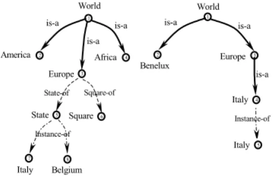
Analysis of attributes. Let us consider Figure 14. On the left we have a graph, which represents an ontology World, where State and Square are attributes of the concept Europe.
State has two sets of items corresponding to Italy and Belgium. On the right we have a
graph, which represents the concept hierarchy World, where the concept Italy is populated with a set of items about Italy. Attributes can be matched with attributes, but also with
concepts. Suppose that we want to match nodes 71 and 42.
Fig. 14. Analysis of attributes
Cupid does not find a match, due to the significant differences in structure of the given graphs. Following semantic matching, in our case, we can notice that we can substitute the
path Europe1:State1:Italy1 with Italy1 (by taking the proper subset of items relating to Italy)
and matching it with Italy2. In this case we obtain C71 = C42
is-a World Luxembourg is-a is-a Netherlands Benelux 2 3 4 1 Belgium World is-a 1 2 World Benelux is-a Europe is-a Italy is-a Italy Instance-of 1 2 3 4 5 Square 1 Square-of Instance-of State is-a State-of World Africa is-a is-a Europe America Belgium Italy 2 3 4 5 6 7 8
4
Implementing Semantic Matching
There are two levels of granularity while performing semantic (and also syntactic match-ing) matching: element-level and structure-level. Element-level matching techniques com-pute mapping elements between individual labels/concepts at nodes; structure-level tech-niques compute mapping elements between subgraphs.
4.1 Element-level Semantic Matching
Element-level semantic techniques analyze individual labels/concepts at nodes. At the element-level we can exploit all the techniques discussed in the literature, see for instance [9], [15], [18]. The main difference here is that, instead of a syntactic similarity measure, these techniques must be modified to return a semantic relation R, as defined in Section 3. We distinguish between weak semantics and strong semantics element-level techniques.
Weak semantics techniques are syntax driven techniques: examples are techniques, which
consider labels as strings, or analyze data types, or soundex of schema elements. Let us consider some examples.
Analysis of strings. String analysis looks for common prefixes or suffixes and calculates the distance between two strings. For example, the fact that the string "phone" is a sub-string of the sub-string "telephone" can be used to infer that "phone" and "telephone" are syno-nyms. Before analyzing strings, a matcher could perform some preliminary parsing, e.g., extract tokens, expand abbreviations, delete articles and then match tokens. The analysis of strings discovers only equality between concepts.
Analysis of data types. These techniques analyze the data types of the elements to be com-pared and are usually performed in combination with string analysis. For example, the elements "phone" and "telephone" are supposed to have the same data type, namely "string" and therefore can be found equal. However, "phone" could also be specified as an "integer" data type. In this case a mismatch is found. As another example the integer "Quantity" is found to be a subset of the real "Qty". This kind of analysis can produce any kind of se-mantic relation.
Analysis of soundex. These techniques analyze elements’ names from how they sound. For example, elements "for you" and "4 U" are different in spelling, but similar in soundex. This analysis can discover only equality between concepts.
Strong semantics techniques exploit, at the element- level, the semantics of labels. These
techniques are based on the use of tools, which explicitly codify semantic information, e.g., thesauruses [14], WordNet [17] or combinations of them [7]. Notice that these techniques are also used in syntactic matching. In this latter case, however, the semantic information is lost before moving to structure-level matching and approximately codified in syntactic relations.
Precompiled thesaurus. A precompiled thesaurus usually stores entries with synonym and hypernym relations. For example, the elements "e-mail" and "email" are treated as syno-nyms from the thesaurus look up: syn key - "e-mail:email = syn". Precompiled thesauruses (most of them) identify equivalence and more general/specific relations. In some cases domain ontologies are used as precompiled thesauruses [16].
WordNet. WordNet is an electronic lexical database for English (and other languages), where various senses (namely, possible meanings of a word or expression) of words are put together into sets of synonyms (synsets). Synsets in turn are organized as hierarchy. Fol-lowing [19] we can define the semantic relations in terms of senses. Equality: one concept is equal to another if there is at least one sense of the first concept, which is a synonym of the second. Overlapping: one concept is overlapped with the other if there are some senses in common. Mismatch: two concepts are mismatched if they have no sense in common.
More general / specific: One concept is more general than the other iff there exists at least
one sense of the first concept that has a sense of the other as a hyponym or as a meronym. One concept is less general than the other iff there exists at least one sense of the first con-cept that has a sense of the other concon-cept as a hypernym or as a holonym. For example, according to WordNet, the concept "hat" is a holonym for the concept "brim", which means that "brim" is less general than "hat".
4.2. Structure-level Semantic Matching
The approach we propose is to translate the matching problem, namely the two graphs and our mapping queries into a propositional formula and then to check it for its validity. By mapping query we mean here the pair of nodes that we think will match and the semantic relation between them. In the following we show how, limited to the case of DAG’s and
is-a hieris-archies, we cis-an check vis-alidity by using SAT. Notice this-at SAT deciders is-are correct
and complete decision procedures for propositional satisfiability and therefore will exhaus-tively check for all possible mappings. Being complete, they automatically implement all the examples described in the previous section, and more. This is another advantage over syntactic matching, whose existing implementations are based only on heuristics.
Our SAT based approach to semantic matching incorporates six steps. We describe below its intended behavior by running these six steps on the example shown in Figure 11 and by
matching nodes 51 and 12 (steps 2-5 are taken from [19]).
1. Extract the two graphs. Notice that during this step, in the case of DB, XML or OODB schemas, it is necessary to extract useful semantic information, for instance in the form of ontologies. There are various techniques for doing this, see for instance [16]. The re-sult is the graph in Figure 11.
2. Compute element-level semantic matching. For each node, compute semantic
rela-tions holding among all the concepts denoted by labels at nodes under consideration. In
this case CA1 has no semantic relation with CC2 while we have that CC1 = CC2.
3. Compute concepts at nodes. Starting from the root of the graph, attach to each node the
concepts of all the nodes above it. Thus, we attach C11 = CA1to node 11; C51= CA1∩CC1to
node 51; C12= CC2 to node 12 in the is-a hierarchy. As it turns out we have that C51⊆ C12.
4. Construct the propositional formula, representing the matching problem. In this step we translate all the semantic relations computed in step 2 into propositional formulas. This is done according to the following transition rules:
Subset translates into implication; equality into equivalence; disjointness into the
nega-tion of conjuncnega-tion. In the case of Figure 11 we have that CC1≡ CC2 is an axiom.
Further-more, since we want to prove that C51⊆ C12, our goal is to prove that ((CA1∧ CC1)→ CC2).
Thus, our target formula is ((CC1≡ CC2) → (CA1∧ CC1)→ CC2)).
5. Run SAT. In order to prove that ((CC1≡ CC2) → (CA1∧ CC1)→ CC2)) is valid, we prove that
its negation is unsatisfiabile, namely that a SAT solver run on the following formula
((CC1≡ CC2) ∧¬ (CA1∧ CC1)→ CC2)) fails. A quick analysis shows that SAT will return
FALSE.
6. Iterations. Iterations are performed re-running SAT. We need iterations, for instance, when matching results are not good enough, for instance no matching is found or a form
of matching is found, which is too weak, and so on1. The idea is to exploit the results
ob-tained during the previous run of SAT to tune the matching and improve the quality of the final outcome. Let us consider Figure 15.
Fig. 15. Not good enough answer
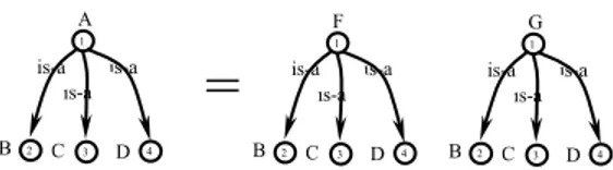
Suppose that we have found out that C21∩ C22 ≠ ∅, and that we want to improve this result.
Suppose that an oracle tells us that CA1 = CF2 ∪ CG2. In this case the graph on the left in
Fig-ure 15 can be transformed into the two graphs in FigFig-ure 16.
Fig. 16. Extraction of additional semantic information
After this additional analysis we can infer that C21= C22. As a particular interesting case,
consider the following situation, see Figure 16.1.
1 [11] provides a long discussion about the importance of dealing with the notion of "good enough
answer" in information coordination in peer-to-peer systems.
CA1 ⊇ CA2 ⇒ CA2 → CA1 CA1⊆ CA2 ⇒ CA1 → CA2 CA1= CA2 ⇒ CA1 ≡ CA2 CA1 ⊥ CA2 ⇒ ¬( CA1 ∧ CA2) is-a is-a A B is-a D C 4 2 3 1 F is-a is-a C B 2 3 1 B C D is-a is-a A is-a 4 3 2 1 B C D is-a is-a F is-a 4 3 2 1 B C D is-a is-a G is-a 4 3 2 1
=
Fig. 16.1. Extraction of additional semantic information. Example
In this case the concept Brussels in the graph on the left (after the sign “=”) becomes in-consistent (empty intersection) and can be omitted; and the same for the concepts at nodes
Amsterdam and Tilburg in the graph on the right. The resulting situation is as follows:
Fig. 16.2. Extraction of additional semantic information. Example
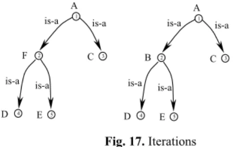
Another motivation for multiple iterations is to use the result of a previous match in order to speed up the search of new matches. Consider the following example.
Fig. 17. Iterations
Having found that C21⊆ C22, we can automatically infer that C51⊆ C52, without rerunning
SAT, for obvious reasons, and the same for C41 and C42. As a particular case consider the
following situation:
Fig. 17.1. Iterations. Example A C F is-a is-a is-a is-a E D 1 5 4 3 2 A C B is-a is-a is-a is-a E D 1 5 4 3 2 is-a is-a Florence Images is-a Toscany 1 2 is-a Asia 3 5 mountains 4 is-a is-a Florence Images is-a Italy 1 2 is-a Asia 3 5 mountains 4 Tilburg Amsterdam Benelux is-a is-a 1 2 3 4 is-a Brussels
=
Tilburg Amsterdam Holland is-a is-a 1 2 3 4 is-aBrussels Amsterdam Tilburg Belgium Brussels is-a is-a 1 2 3 4 is-a Tilburg Amsterdam Benelux is-a is-a 1 2 3 4 is-a Brussels
=
Tilburg Amsterdam Holland is-a is-a 1 2 3 Belgium Brussels 1 4 is-aOur algorithm allows us to find that C51 ⊆ C52, while, being Tuscany in Italy we actually
have C51 = C52. This is an acceptable result as long as we are not looking for the strongest
possible relation holding between two nodes.
5 Related
Work
From a technical point of view the matcher we have proposed in this paper is a function
Match_Nodes_R(G1,G2, n1, n2, R) which takes two graphs, two nodes, and a relation and
returns a Yes/No answer. Most matchers proposed in the literature are a function Match(G1,
G2) which takes two graphs and returns a set of mappings (n1, n2, R). However, it is easy to
see how we can build an analogous function. The naive approach being to triple loop on the nodes of the graphs and on the set of proposed relations and, at each loop, call
Match_Nodes_R.
At present, there exists a line of semi-automated schema matching and ontology integration systems, see for instance [14], [9], [13], [7], [1], [16], [8], etc. Most of them implement syntactic matching. A good survey, up to 2001, is provided in [18]. The classification given in this survey distinguishes between individual implementations of match and combinations of matchers. Individual matchers comprise instance- and schema-level, element- and struc-ture-level, linguistic- and constrained-based matching techniques. Individual matchers can be used in different ways, e.g. simultaneously (hybrid matchers), see [13], [7], [14] or in series (composite matchers), see for instance [8], [9].
The idea of generic (syntactic) matching was first proposed by Phil Bernstein and imple-mented in the Cupid system [14]. Cupid implements a complicated hybrid match algorithm comprising linguistic and structural schema matching techniques, and computes normalized similarity coefficients with the assistance of a precompiled thesaurus. COMA [9] is a ge-neric schema matching tool, which implements more recent composite gege-neric matchers. With respect to Cupid, the main innovation seems to be a more flexible architecture. COMA provides an extensible library of matching algorithms; a framework for combining obtained results, and a platform for the evaluation of the effectiveness of the different matchers.
A lot of state of the art syntactic matching techniques exploiting weak semantic element-level matching techniques have been implemented. For instance, in COMA, schemas are internally encoded as DAGs, where the elements are the paths, which are analyzed using string comparison techniques. Similar ideas are exploited in Similarity Flooding (SF) [15]. SF is a hybrid matching algorithm based on the ideas of similarity propagation. Schemas are presented as directed labeled graphs; the algorithm manipulates them in an iterative fix-point computation to produce mappings between the nodes of the input graphs. The tech-nique uses a syntactic string comparison mechanism of the vertices’ names to obtain an initial mapping, which is further refined within the fix-point computation.
Some work has also been done in strong semantics element-level matching. For example, [7] utilizes a common thesaurus, while [14] has a precompiled thesaurus. In MOMIS [7], [2] element-level matching using a common thesaurus is carried out through a calculation of the name, structural and global affinity coefficients. The thesaurus presents a set of
in-tensional and exin-tensional relations, which depict intra- and inter-schema knowledge about classes, and attributes of the input schemas. The common thesaurus is built using WordNet and ODB-Tools [4]. All these systems implement syntactic matching and, when moving from element-level to structure-level matching, don’t exploit the semantic information residing in the graph structure, and just translate the element-level semantic information into affinity levels.
As far as we know the only example where element-level and a simplified version of struc-ture- level strong semantics matching have been applied is CTXmatch [19]. In this work SAT is used as the basic inference engine for structure-level matching. The main problem of CTXmatch is that its rather limited in scope (it applies only to concept hierarchies), and it is hard to see the general lessons behind this work. For instance, the authors have made no attempt to do a thorough comparison of their approach with the other matching tech-niques, or to highlight its strengths and weaknesses. This paper provides the basics for a better understanding of the work on CTXmatch.
6 Conclusions
In this paper we have stated and analyzed the major matching problems e.g., matching database schemas, XML schemas, conceptual hierarchies and ontologies and shown how all these problems can be defined as a more generic problem of matching graphs. We have identified semantic matching as a new approach for performing generic matching, and discussed some of its key properties. Finally, we have identified SAT as a possible way of implementing semantic matching, and proposed an iterative semantic matching approach based on SAT.
This is only very preliminary work, some of the main issues we need to work on are: de-velop an efficient implementation of the system, do a thorough testing of the system, also against the other state of the art matching systems, study how to take into account attributes and instances, analyze how to extract semantics from schemas (also taking into account integrity constraints), and so on.
Acknowledgments
Thanks to Luciano Serafini, Paolo Bouquet, Bernardo Magnini for many discussions on CTXmatch. Stefano Zanobini and Phil Bernstein have proposed very useful feedback on the semi-final version of this paper. Also thanks to Mikalai Yatskevich for his work on running SAT solvers on our matching problems.
References
1. Arens, Y, Hsu, C and Knoblock, CA, 1996, “Query processing in the SIMS information mediator” In Austin Tate editor, Advanced Planning Technology AAAI Press.
2. Bergamaschi, S, Castano, S and Vincini, M, 1999, “Semantic Integration of Semistruc-tured and StrucSemistruc-tured Data Sources” SIGMOD Record 28(1) 54-59.
3. Bernstein, P, Giunchiglia, F, Kementsietsidis, A, Mylopoulos, J, Serafini, L and Zaihrayeu I, 2002, “Data Management for Peer-to-Peer Computing: A Vision” Proceedings of work-shop on WebDB 89-94.
4. Beneventano, D, Bergamaschi, S, Lodi, S and Sartori, C, 1998, “Consistency checking in complex object database schemata with integrity constraints” IEEE Transactions on Knowledge and Data Engineering 10(4) 576-598.
5. Buneman, P, Davidson, S, Hillebrand, G and Suciu, D, 1996, “A Query Language And Optimization Techniques For Unstructured Data” Proceedings of ACM SIGMOD 505-516. 6. Buneman, P, 1997, “Semistructured data”. Proceedings of PODS 117–121.
7. Castano, S, De Antonellis, V and Vimercati, S, 2001, “Global Viewing of Heterogeneous Data Sources” IEEE Transactions on Knowledge and Data Engineering 13(2) 277-297. 8. Doan, A, Madhavan, J, Domingos, P and Halvey, A, 2002, “Learning to map between
ontologies on the semantic web” Proceedings of WWW 662-673.
9. Do, HH and Rahm, E, 2002, “COMA – A System for Flexible Combination of Schema Matching Approaches” Proceedings of VLDB 610-621.
10. Goh, CH, 1997, “Representing and Reasoning about Semantic Conflicts in Heterogeneous Information Sources” Ph.D. thesis, MIT.
11. Giunchiglia, F and Zaihrayeu, I, 2002, “Making peer databases interact - a vision for an architecture supporting data coordination” Proceedings of workshop on CIA 18-35.
12. Halevy, A, 2001, “Answering queries using views: a survey” VLDB Journal 10(4) 270-294.
13. Li, W and Clifton, C, 2000, “SEMINT: A tool for identifying attribute correspondences in heterogeneous databases using neural networks” Data and Knowledge Engineering
33(1) 49-84.
14. Madhavan, J, Bernstein, P and Rahm, E, 2001, ”Generic schema matching with Cupid” Proceedings of VLDB 49-58.
15. Melnik, S, Garcia-Molina, H and Rahm, E, 2002, “Similarity Flooding: A Versatile Graph Matching Algorithm” Proceedings of ICDE 117-128.
16. Mena, E, Kashyap, V, Sheth, A and Illarramendi, A, 1996, “Observer: An approach for query processing in global information systems based on interoperability between pre-existing ontologies” Proceedings of CoopIS 14-25.
17. Miller, AG, 1995, “Wordnet: A lexical database for English” Communications of the ACM 38(11) 39-41.
18. Rahm, E and Bernstein, P, 2001, “A survey of approaches to automatic schema matching” VLDB Journal 10(4) 334-350.
19. Serafini, L, Bouquet, P, Magnini, B and Zanobini, S, 2003, “An Algorithm for Matching Contextualized Schemas via SAT”, IRST Technical Report 0301-06, Istituto Trentino di Cultura.
20. Wache, H, Voegele, T, Visser, U, Stuckenschmidt, H, Schuster, G, Neumann, H and Huebner, S, 2001, “Ontology-based integration of information - a survey of existing ap-proaches”. Procedings of workshop on Ontologies and Information Sharing at IJCAI 108-117.
21. Zhang, K and Shasha, D, 1997, “Approximate Tree Pattern Matching” in A. Apostolico and Z. Galil (eds.) Pattern Matching in Strings, Trees, and Arrays Oxford University Press.