Institut de Recerca en Economia Aplicada Regional i Pública Document de Treball 2018/05 1/24 pág. Research Institute of Applied Economics Working Paper 2018/05 1/24 pág.
“A regional perspective on the accuracy of machine learning
forecasts of tourism demand based on data characteristics”
Oscar Claveria, Enric Monte and Salvador Torra4
WEBSITE: www.ub.edu/irea/ • CONTACT: [email protected]
The Research Institute of Applied Economics (IREA) in Barcelona was founded in 2005, as a research institute in applied economics. Three consolidated research groups make up the institute: AQR, RISK and GiM, and a large number of members are involved in the Institute. IREA focuses on four priority lines of investigation: (i) the quantitative study of regional and urban economic activity and analysis of regional and local economic policies, (ii) study of public economic activity in markets, particularly in the fields of empirical evaluation of privatization, the regulation and competition in the markets of public services using state of industrial economy, (iii) risk analysis in finance and insurance, and (iv) the development of micro and macro econometrics applied for the analysis of economic activity, particularly for quantitative evaluation of public policies.
IREA Working Papers often represent preliminary work and are circulated to encourage discussion. Citation of such a paper should account for its provisional character. For that reason, IREA Working Papers may not be reproduced or distributed without the written consent of the author. A revised version may be available directly from the author.
Any opinions expressed here are those of the author(s) and not those of IREA. Research published in this series may include views on policy, but the institute itself takes no institutional policy positions.
Abstract
In this work we assess the role of data characteristics in the accuracy of machine learning (ML) tourism forecasts from a spatial perspective. First, we apply a seasonal-trend decomposition procedure based on non-parametric regression to isolate the different components of the time series of international tourism demand to all Spanish regions. This approach allows us to compute a set of measures to describe the features of the data. Second, we analyse the performance of several ML models in a recursive multiple-step-ahead forecasting experiment. In a third step, we rank all seventeen regions according to their characteristics and the obtained forecasting performance, and use the rankings as the input for a multivariate analysis to evaluate the interactions between time series features and the accuracy of the predictions. By means of dimensionality reduction techniques we summarise all the information into two components and project all Spanish regions into perceptual maps. We find that entropy and dispersion show a negative relation with accuracy, while the effect of other data characteristics on forecast accuracy is heavily dependent on the forecast horizon.
JEL Classification: C45; C51; C53; C63; E27; L83.
Keywords:STL decomposition; non-parametric regression; time series features; forecast accuracy; machine learning; tourism demand; regional analysis.
Oscar Claveria AQR-IREA, University of Barcelona (UB). Tel.: +34-934021825; Fax.: +34-934021821. Department of Econometrics, Statistics and Applied Economics, University of Barcelona, Diagonal 690, 08034 Barcelona, Spain. E-mail address: [email protected]
Enric Monte. Department of Signal Theory and Communications, Polytechnic University of Catalunya (UPC)
Salvador Torra. Riskcenter-IREA, Department of Econometrics and Statistics, University of Barcelona (UB)
Acknowledgements
This research was supported by by the projects ECO2016-75805-R and TEC2015-69266-P from the Spanish Ministry of Economy and Competitiveness.
1. Introduction
The increasing weight of the tourism industry in the gross domestic product of most countries explains the growing interest in the sector from economic circles. Bilen et al. (2015), Brida et al. (2016), Chou (2013), Soukiazis and Proença (2008) and Tang and Abosedra (2016) have recently analysed the relevance of tourism in economic growth. The continuous rise of tourism demand highlights the importance of correctly anticipating the number of arrivals at the destination level. The refinement of tourism demand forecasts has led to an extensive body of research, but in most of these studies data characteristics are overlooked (Kim and Schwartz, 2013).
The main objective of this work is to fill this gap. With this aim we analyse the effect of time series features of international tourist arrivals to the different Spainsh regions on the forecast accuracy derived from a multiple-step-ahead forecasting evaluation. Spain is one of the world’s top tourist destinations after France and the United States. The country received more than 86 million tourist arrivals in 2017, which represents an 8.9% increase in relation to 2016 (Spanish Statistical Office – http://www.ine.es). As a result, Spain has become the world’s second most important destination after France. The fact that regional markets present marked differences and have evolved in very diverse forms, has led us to conduct the analysis at a regional level.
The search for more accurate predictions explains that statistical learning methods based on artificial intelligence (AI) are being increasingly used with forecasting purposes. Machine learning (ML) belongs to a subfield of AI that is based on the construction of algorithms that learn through experience. The most commonly used AI-based techniques for prediction are support vector regression (SVR), which can be regarded as an extension of the support vector machine (SVM) mechanism, and neural networks (NNs). In recent years, several authors have found evidence in favour of SVRs and NNs when compared to more traditional time series models (Akin, 2015; Chen and Wang, 2007; Claveria and Torra, 2014; Hong et al., 2011; Xu et al., 2016).
In this study we compare the time series features of tourist arrivals to Spain to the forecasting performance of several ML methods. On the one hand, with the aim of assessing the role of time series features in the accuracy of ML tourism predictions, we use a seasonal-trend decomposition procedure based on non-parametric regression to isolate the different components of the time series of international tourism demand to all Spanish regions and compute a set of measures to describe the features of the data.
On the other hand, we design a recursive multiple-step-ahead forecasting experiment to evaluate the accuracy of the predictions obtained with the different techniques. Specifically, we compare the forecast accuracy obtained with a Gaussian process regression (GPR) model to that of several SVR and NN models. GPR is a statistical learning technique originally devised for spatial interpolation, which has recently been used for time series forecasting (Ben Taieb et al., 2010). Finally, by means of dimensionality reduction techniques we evaluate the interactions between data characteristics of the different regions and the obtained accuracy for different forecast horizons.
The study is organized as follows. The next section reviews the existing literature on tourism demand forecasting with ML methods. In section three, we first describe the data and compute a set of time series features, then we assess the predictive performance of the models in a multiple-step-ahead forecasting experiment in order to evaluate the role of time series features in the accuracy of the predictions by means of a multivariate analysis. Concluding remarks and the potential lines for future research are provided in the last section.
2. Literature Review
There is a growing body of literature about tourism demand forecasting. See Li et al. (2005), Peng et al. (2014) , Song and Li (2008) and Witt and Witt (1995) for a thorough review of tourism demand forecasting studies. Most of this research is based on causal econometric models (Cortés-Jiménez and Blake, 2011; Gunter and Önder, 2015; Lin et al., 2015; Tsui et al., 2014), or on traditional time series models (Assaf et al., 2011; Chu, 2009; Gounopoulos et al., 2012; Li et al., 2013). However, the complex data generating process of tourism demand has fostered the use of nonlinear approaches for tourism forecasting.
In this context, ML methods are experiencing a growing use (Zhang and Zhang, 2014). The first AI-based method implemented for tourism demand forecasting were NNs. There are many NN models. The first and most commonly used NN architecture in tourism demand forecasting is the multi-layer perceptron (MLP) (Burger et al., 2001; Claveria and Torra, 2014; Hassani et al., 2015; Kon and Turner, 2005; Law, 2000; Lin et al., 2011; Molinet et al., 2015; Padhi and Aggarwal, 2011; Palmer et al., 2006; Pattie and Snyder, 1996; Teixeira and Fernandes, 2012; Tsaur et al., 2002; Uysal and El Roubi, 1999).
MLP are feed-forward networks in which the information runs only in one direction, while in recurrent networks there are bidirectional data flows (Cho, 2003). A special class of feed-forward architecture with two layers of processing is the radial basis function (RBF). The first study to implement a RBF architecture for forecasting tourism demand was that of Kon and Turner (2005), who used a RBF NN to forecast arrivals to Singapore. Cang (2014) generated predictions of UK inbound tourist arrivals and combined them in nonlinear models. Çuhadar et al. (2014) compared the forecasting performance of RBF and MLP NNs to predict cruise tourist demand at the destination level (Izmir, Turkey).
The first implementations of SVMs for tourism demand forecasting were those of Pai and Hong (2005) and Hong (2006), who used SVMs to forecast tourist arrivals to Barbados. The recent extension of the SVM mechanism to regression analysis has fostered the use of SVR models for tourism prediction. Chen and Wang (2007) generated forecasts of tourist arrivals to China with SVR, back propagation NN and autoregressive integrated moving average (ARIMA) models, obtaining the best forecasting results with SVRs. Hong et al. (2011) also obtained more accurate forecasts with SVRs than with ARIMA models. Akin (2015) compared the forecasting results of SVR to that of ARIMA and NN models to predict international tourist arrivals to Turkey, and found that SVR outperformed NNs in all cases, but ARIMA models only when the slope feature was more prominent.
The works of Smola and Barlett (2001), MacKay (2003), and Rasmussen and Williams (2006) have been key in the development of GPR, which can be regarded as a statistical learning method for interpolation. By expressing the model in a Bayesian framework, GPR applications can be extended beyond spatial interpolation to regression problems. From a wide range of ML methods, Ahmed et al. (2010) found that NN and GPR models showed the best forecasting performance on the monthly M3 time series competition data. In a similar exercise, Andrawis et al. (2011) found evidence in favour of a simple average combination of NN, GPR and linear models for the NN5 competition.
Nevertheless, there are very few studies that implement GPR for tourism forecasting (Claveria et al., 2016a,b; Wu et al., 2012). Claveria et al. (2016b) proposed an extension of the GPR model for multiple-input multiple-ouput forecasting.Wu et al. (2012) used a sparse GPR model to predict tourism demand to Hong Kong, obtaining better forecasting results than with autoregressive moving average (ARMA) and SVR models.
The first attempt to use statistical learning process for tourism demand forecasting in Spain was that of Palmer et al. (2006), who applied a MLP NN to forecast tourism expenditure in the Balearic Islands. Medeiros et al. (2008) developed a NN-generalized
autoregressive conditional heteroscedasticity model to estimate demand for international tourism to the Balearic Islands. Claveria et al. (2015) compared the performance of three NN architectures in a multiple-input multiple-output setting for generating predictions of tourist arrivals to Catalonia (Spain) from all visitors markets simultaneously, finding tha RBF networks provided better forecasting results than the MLP and Elman architectures.
As a result of a comprehensive meta-analysis of recent tourism studies, Kim and Schwartz (2013) have pointed out that the growing interest in refining tourism predictions has not been matched by a similar effort in analysing the effect of data characteristics on forecasting results. To cover this deficit, in this work we aim to shed some light on this issue by focusing on time series features and ML forecasts.
3. Time Series Features
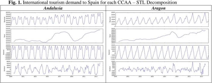
In this section we describe the characteristics of the individual series on international tourism demand to each of the regions of Spain. Data is obtained from the Spanish Statistical Office (National Statistics Institute – INE – www.ine.es) and include the monthly number of tourist arrivals at a regional level over the time period 1999:01 to 2014:03. With the aim of computing time series features, we first apply the “Seasonal and Trend Decomposition using Loess” (STL) procedure proposed by Cleveland et al. (1990) to decompose the seasonal and trend comopnents of the time series. Loess is a locally weighted polynomial regression method originally devised by Cleveland (1979).
STL presents several advantages over the classical decomposition method and X-12-ARIMA: it can handle any type of seasonality, the seasonal component is allowed to change over time, the smoothness of the trend-cycle can be controlled, and it can be robust to outliers (Bergmeir et al., 2016; Hyndman et al., 2016). Given that Yt Tt St Rt, where
t
T denotes the trend component, St the seasonal component and Rt the residual, we can assess the strength of each component by computing:
t t t S Y V R V 1 trend of strength (1) t t t T Y V R V 1 y seasonalit of strength (2) We also compute the skewness, the kurtosis, the coefficient of variation, the first autocorrelation (r1), and two additional statistics: the Box-Cox lambda (1) and spectral
The lambda value indicates the power to which all data should be raised in order to be normally distributed (Box and Cox, 1964). The Box-Cox power transformation searches within the interval [-5;5] until the optimal value is found in:
0 if log 0 if 1 1 2 1 1 2 1 t t t Y Y Y (3)Spectral entropy describes the complexity of a system and can be used as a proxy for the predictability of a given time series. Rosselló and Sansó (2017) have recently showed the appropriateness of entropy as a new information tool for tourism seasonality analysis.
H can be computed as:
f f d
H y log y (4)
Where fy
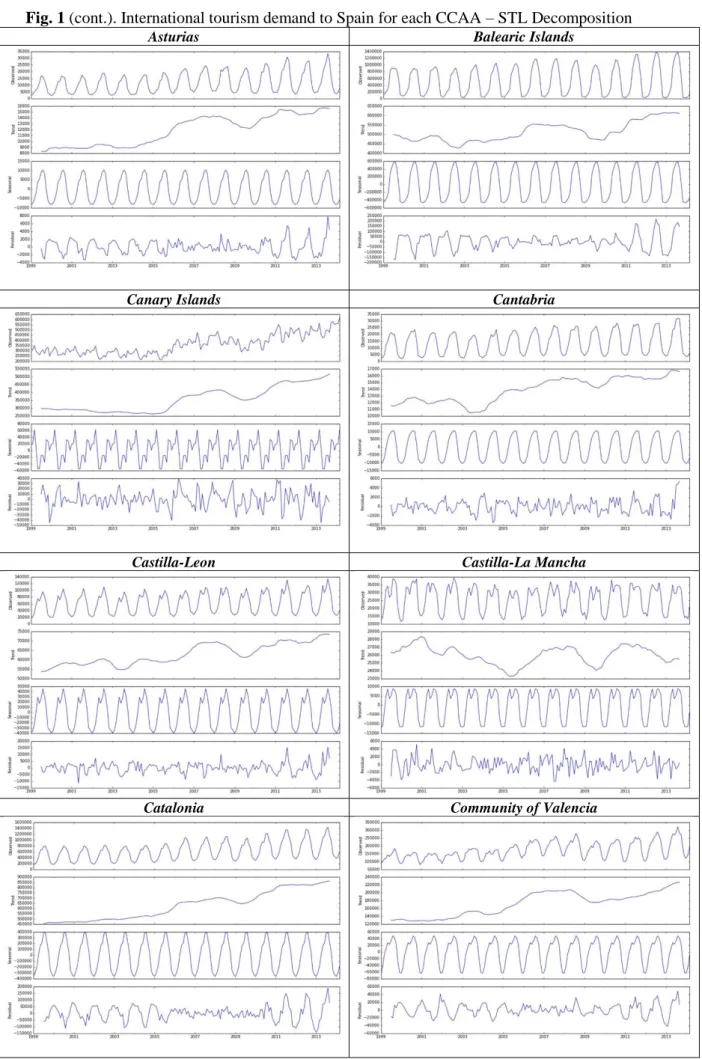
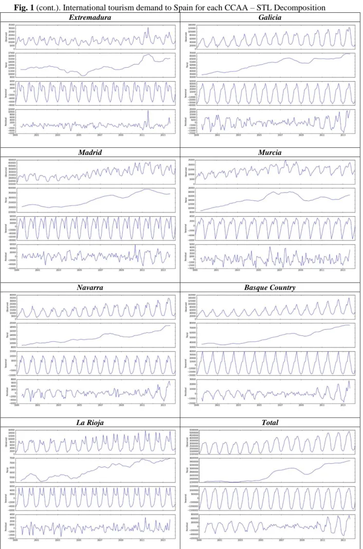
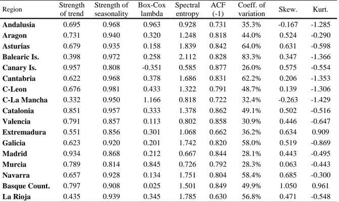
is the spectral density of Yt. Low values of H are indicative of more signal, suggesting that a time series is easier to forecast (Hyndman et al., 2016).In Fig. 1 we graph the evolution of tourist arrivals in each region from 1999 to 2014, including the three components obtained through STL decomposition. In Table 1 we present the descriptive analysis of the data. We can observe how the time series features notedly vary across regions. The Canary Islands present the highest level of strength of trend, but the lowest in terms of the strength of seasonality, Box-Cox lambda, and spectral entropy. On the other hand, the Balearic Islands present the highest values of entropy and dispersion.
Fig. 1. International tourism demand to Spain for each CCAA – STL Decomposition
Fig. 1 (cont.). International tourism demand to Spain for each CCAA – STL Decomposition
Asturias Balearic Islands
Canary Islands Cantabria
Castilla-Leon Castilla-La Mancha
Fig. 1 (cont.). International tourism demand to Spain for each CCAA – STL Decomposition
Extremadura Galicia
Madrid Murcia
Navarra Basque Country
Table 1 Descriptive analysis of foreign tourist arrivals (1999:09-2013:09) Region Strength of trend Strength of seasonality Box-Cox lambda Spectral entropy ACF (-1) Coeff. of
variation Skew. Kurt.
Andalusia 0.695 0.968 0.963 0.928 0.731 35.3% -0.167 -1.285 Aragon 0.731 0.940 0.320 1.248 0.818 44.0% 0.524 -0.290 Asturias 0.679 0.935 0.158 1.839 0.842 64.0% 0.631 -0.598 Balearic Is. 0.398 0.972 0.258 2.112 0.828 83.3% 0.347 -1.366 Canary Is. 0.957 0.808 -0.351 0.585 0.877 26.0% 0.575 -0.554 Cantabria 0.622 0.968 0.378 1.686 0.831 62.2% 0.206 -1.353 C-Leon 0.676 0.981 0.433 1.322 0.791 48.7% 0.139 -1.306 C-La Mancha 0.332 0.950 1.166 0.818 0.722 32.4% -0.263 -1.429 Catalonia 0.851 0.957 0.333 1.378 0.862 49.1% 0.502 -0.516 Valencia 0.791 0.857 0.113 0.802 0.858 30.9% 0.446 -0.647 Extremadura 0.551 0.856 0.301 1.068 0.662 36.2% 0.634 0.909 Galicia 0.623 0.920 0.201 1.742 0.820 58.0% 0.519 -0.869 Madrid 0.934 0.868 0.212 0.667 0.844 28.1% 0.443 -0.495 Murcia 0.789 0.814 0.845 0.726 0.792 28.3% 0.063 -0.443 Navarra 0.657 0.928 0.134 1.751 0.804 58.4% 0.685 -0.300 Basque Count. 0.797 0.908 0.025 1.501 0.849 49.9% 1.050 0.961 La Rioja 0.435 0.939 0.345 1.785 0.630 56.8% 0.471 -0.548 Notes: Basque Count. stands for Basque Country, C-Leon stands for Castilla-Leon, C-La Mancha stands for Castilla-La Mancha. Coeff. of variation denotes Coefficient of variation; ACF (-1) the first autocorrelation;. Skew., Skewness; and Kurt., Kurtosis.
Next, we compute the forecast accuracy of the different ML models: a GPR, a linear and a polynomial SVR, and MLP and RBF NN architectures. The theoretical foundation of the GPR model (Matheron, 1973) is based on previous geostatistic research by Krige (1951). Comprehensive information about GPR can be found in Rasmussen and Williams (2006). A GPR can be regarded as a method of interpolation based on the assumption that the inputs have a joint multivariate Gaussian distribution characterized by an analytical model of the structure of the covariance matrix (Williams and Rasmussen, 1996). As GPRs allow specifying the functional form of the covariance functions, in this experiment we use a radial basis kernel with a linear trend to account for the trend component present in most of the time series over the training period. Alternative sets of kernels are discussed in MacKay (2003). See Claveria et al. (2016a.,b) and Wu et al. (2012) for a detailed description of the model used in this study.
The SVR mechanism was proposed by Drucker et al. (1997) and can be regarded as an extension of SVMs to construct data-driven and nonlinear regressions. The original SVM algorithm was developed by Vapnik (1995) and Cortes and Vapnik (1995). For a comprehensive presentation of SVR models see Cristianini and Shawhe-Taylor (2000). The objective of a SVR is to define an approximation of the regression function within a tube generated by means of a set of support vectors that belong to the training data set. This
is done by introducing restrictions on the structure or curvature of the set of functions over which the estimation is done (Vapnik, 1998; Schölkopf and Smola, 2002). Any function satisfying Mercer’s condition (Vapnik, 1995) can be used as the kernel function. In this experiment we use both a linear and a polynomial kernel for the estimation of the regression. See Chen and Wang (2007) and Hong et al. (2011) for a detailed description of the model.
NN models are used to identify related spatial and temporal patterns by learning from experience. A complete summary on the use of NNs with forecasting purposes can be found in Zhang et al. (1998). In this study we use two NN models: MLP and RBF. See Claveria et al. (2017a) for a detailed description of the models applied. In this experiment, we have used the Levenberg-Marquardt algorithm to estimate the parameters of the networks.
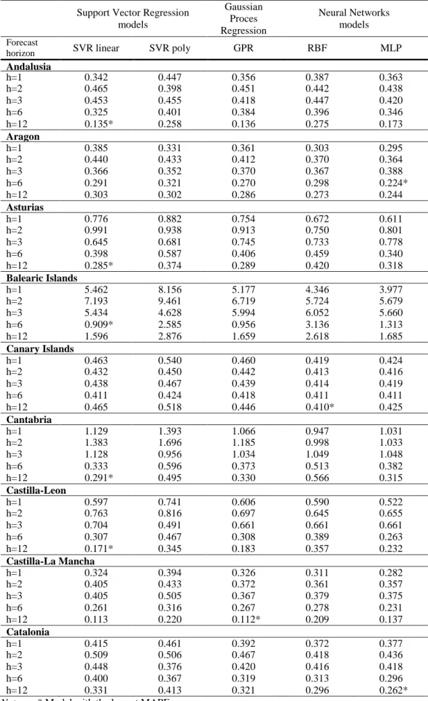
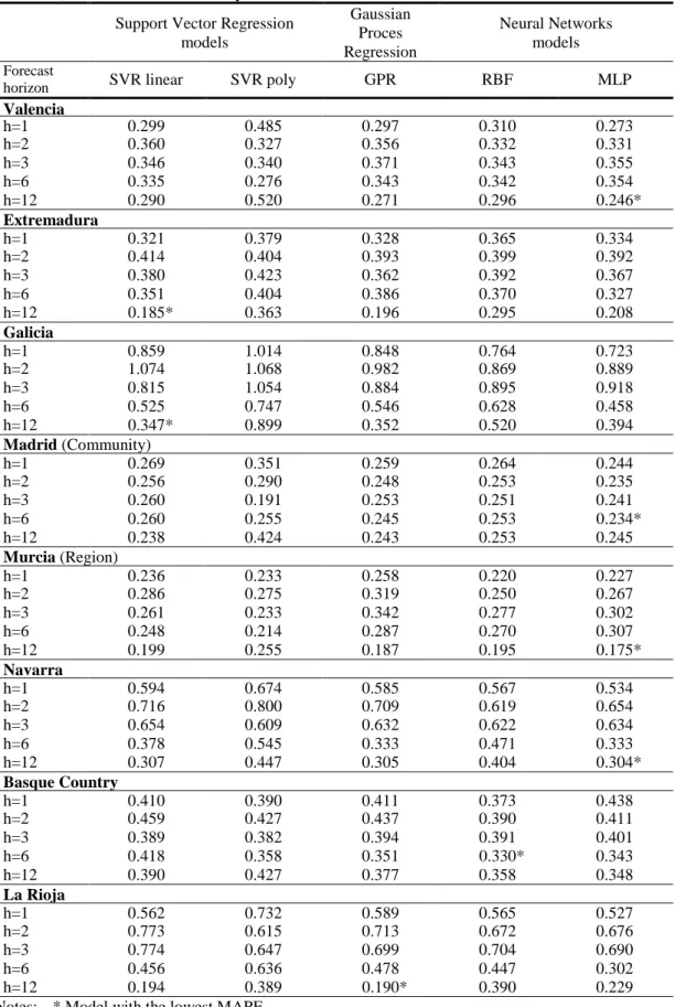
The first 52% of the observations were used as the initial training set, the next 33% as the validation set, and and the last 15% as the test set. This partition is done sequentially. The estimation of the models is done recursively for different forecast horizons (1, 2, 3, 6 and 12 months) during the out-of-sample period (2013:01-2014:01). Forecast accuracy results are summarized by means of the Mean Absolute Percentage Error (MAPE). The results of the forecasting experiment are presented in Table 2.
Regarding the different models, we find that the MLP NN model shows lower MAPE values than the rest of the models in 40% of the cases. For one- and six-month ahead forecasts, this percentage goes up to 59% and 65% respectively. Nevertheless, for three-month ahead forecasts the MLP never outperforms the rest of the models, being the polynomial SVR the model that presents the lowest MAPE values in 65% of the cases.
The lowest MAPE in each region is usually obtained either with the MLP NN or the linear SVR. The exceptions are Castilla-La Mancha and La Rioja, where the GPR outperforms the rest of the models, and the Basque Country and the Canary Islands, where the RBF NN generates the forecasts with the lowest MAPE values. In the Canary Islands the RBF outperforms all the other methods for all forecast horizons.
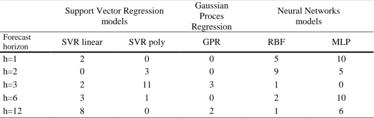
Results of the forecasting experiment are summarized in Table 3, where we present the number regions in which each model provides the lowest MAPE. The results show that the MLP NN outperforms the rest of the models in most of the regions, and both for one- and six-month ahead forecasts.
Table 2. Forecast accuracy. MAPE (2013:01-2014:01) Support Vector Regression
models Gaussian Proces Regression Neural Networks models Forecast
horizon SVR linear SVR poly GPR RBF MLP
Andalusia a h=1 0.342 0.447 0.356 0.387 0.363 h=2 0.465 0.398 0.451 0.442 0.438 h=3 0.453 0.455 0.418 0.447 0.420 h=6 0.325 0.401 0.384 0.396 0.346 h=12 0.135* 0.258 0.136 0.275 0.173 Aragon h=1 0.385 0.331 0.361 0.303 0.295 h=2 0.440 0.433 0.412 0.370 0.364 h=3 0.366 0.352 0.370 0.367 0.388 h=6 0.291 0.321 0.270 0.298 0.224* h=12 0.303 0.302 0.286 0.273 0.244 Asturias h=1 0.776 0.882 0.754 0.672 0.611 h=2 0.991 0.938 0.913 0.750 0.801 h=3 0.645 0.681 0.745 0.733 0.778 h=6 0.398 0.587 0.406 0.459 0.340 h=12 0.285* 0.374 0.289 0.420 0.318 Balearic Islands h=1 5.462 8.156 5.177 4.346 3.977 h=2 7.193 9.461 6.719 5.724 5.679 h=3 5.434 4.628 5.994 6.052 5.660 h=6 0.909* 2.585 0.956 3.136 1.313 h=12 1.596 2.876 1.659 2.618 1.685 Canary Islands h=1 0.463 0.540 0.460 0.419 0.424 h=2 0.432 0.450 0.442 0.413 0.416 h=3 0.438 0.467 0.439 0.414 0.419 h=6 0.411 0.424 0.418 0.411 0.411 h=12 0.465 0.518 0.446 0.410* 0.425 Cantabria a h=1 1.129 1.393 1.066 0.947 1.031 h=2 1.383 1.696 1.185 0.998 1.033 h=3 1.128 0.956 1.034 1.049 1.048 h=6 0.333 0.596 0.373 0.513 0.382 h=12 0.291* 0.495 0.330 0.566 0.315 Castilla-Leon h=1 0.597 0.741 0.606 0.590 0.522 h=2 0.763 0.816 0.697 0.645 0.655 h=3 0.704 0.491 0.661 0.661 0.661 h=6 0.307 0.467 0.308 0.389 0.263 h=12 0.171* 0.345 0.183 0.357 0.232 Castilla-La Mancha h=1 0.324 0.394 0.326 0.311 0.282 h=2 0.405 0.433 0.372 0.361 0.357 h=3 0.405 0.505 0.367 0.379 0.375 h=6 0.261 0.316 0.267 0.278 0.231 h=12 0.113 0.220 0.112* 0.209 0.137 Catalonia a h=1 0.415 0.461 0.392 0.372 0.377 h=2 0.509 0.506 0.467 0.418 0.436 h=3 0.448 0.376 0.420 0.416 0.418 h=6 0.400 0.367 0.319 0.313 0.296 h=12 0.331 0.413 0.321 0.296 0.262*
Table 2 (cont.). Forecast accuracy. MAPE (2013:01-2014:01) Support Vector Regression
models Gaussian Proces Regression Neural Networks models Forecast
horizon SVR linear SVR poly GPR RBF MLP
Valencia h=1 0.299 0.485 0.297 0.310 0.273 h=2 0.360 0.327 0.356 0.332 0.331 h=3 0.346 0.340 0.371 0.343 0.355 h=6 0.335 0.276 0.343 0.342 0.354 h=12 0.290 0.520 0.271 0.296 0.246* Extremadura h=1 0.321 0.379 0.328 0.365 0.334 h=2 0.414 0.404 0.393 0.399 0.392 h=3 0.380 0.423 0.362 0.392 0.367 h=6 0.351 0.404 0.386 0.370 0.327 h=12 0.185* 0.363 0.196 0.295 0.208 Galicia h=1 0.859 1.014 0.848 0.764 0.723 h=2 1.074 1.068 0.982 0.869 0.889 h=3 0.815 1.054 0.884 0.895 0.918 h=6 0.525 0.747 0.546 0.628 0.458 h=12 0.347* 0.899 0.352 0.520 0.394 Madrid (Community) h=1 0.269 0.351 0.259 0.264 0.244 h=2 0.256 0.290 0.248 0.253 0.235 h=3 0.260 0.191 0.253 0.251 0.241 h=6 0.260 0.255 0.245 0.253 0.234* h=12 0.238 0.424 0.243 0.253 0.245 Murcia (Region) h=1 0.236 0.233 0.258 0.220 0.227 h=2 0.286 0.275 0.319 0.250 0.267 h=3 0.261 0.233 0.342 0.277 0.302 h=6 0.248 0.214 0.287 0.270 0.307 h=12 0.199 0.255 0.187 0.195 0.175* Navarra h=1 0.594 0.674 0.585 0.567 0.534 h=2 0.716 0.800 0.709 0.619 0.654 h=3 0.654 0.609 0.632 0.622 0.634 h=6 0.378 0.545 0.333 0.471 0.333 h=12 0.307 0.447 0.305 0.404 0.304* Basque Country h=1 0.410 0.390 0.411 0.373 0.438 h=2 0.459 0.427 0.437 0.390 0.411 h=3 0.389 0.382 0.394 0.391 0.401 h=6 0.418 0.358 0.351 0.330* 0.343 h=12 0.390 0.427 0.377 0.358 0.348 La Rioja h=1 0.562 0.732 0.589 0.565 0.527 h=2 0.773 0.615 0.713 0.672 0.676 h=3 0.774 0.647 0.699 0.704 0.690 h=6 0.456 0.636 0.478 0.447 0.302 h=12 0.194 0.389 0.190* 0.390 0.229
Table 3. Out-of-sample forecast accuracy. Summary Support Vector Regression
models Gaussian Proces Regression Neural Networks models Forecast
horizon SVR linear SVR poly GPR RBF MLP
h=1 2 0 0 5 10
h=2 0 3 0 9 5
h=3 2 11 3 1 0
h=6 3 1 0 2 10
h=12 8 0 2 1 6
Summarizing, we find that:
There are significant differences across regions regarding forecast accuracy.
The MLP NN outperforms the rest models in most of the regions, as opposed to the GPR.
The linear SVR relatively improves its forecasting performance for longer forecast horizons (six- and twelve-month ahead predictions), as opposed to the RBF NN. Regardless of the ML method, forecast accuracy improves for longer horizons. Claveria
et al. (2017b) obtained similar results when comparing GPR to NN models.
With the aim of analysing the effects of data characteristics on forecast accuracy, we link the resuls of the two previous analysis: the time series features (Table 1) and the forecasting results (Table 2). Following the multivariate positioning approach proposed by Claveria (2016), we first rank each region according to its data charateristics and its MAPE values in increasing order. These rankings are then used as the input for an ordinal multivariate analysis that allows us to synthesise all the information in order to evaluate the effect of time series features on forecast accuracy.
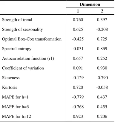
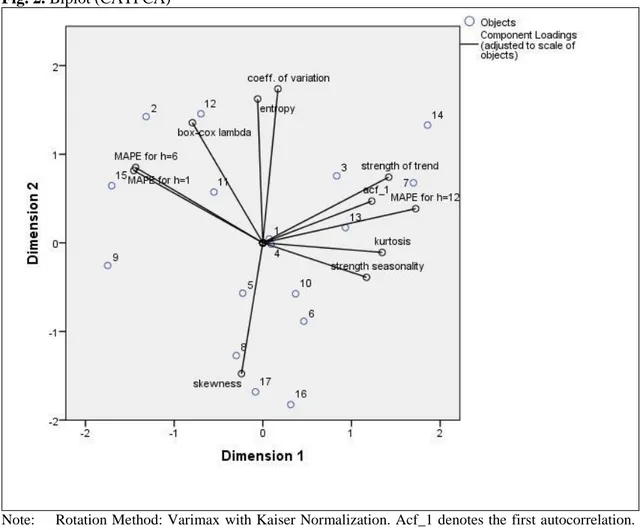
Multivariate techniques for dimensionality reduction have been widely used in tourism studies. The principal components analysis (PCA) framework has been progressively extended to deal with nonlinear relationships in data and with qualitative information. Categorical principal components analysis (CATPCA) can be regarded as a development of PCA (Meulman et al., 2012). See Gifi (1990) for a historical overview, and Linting et al. (2007) for an exhaustive treatment of nonlinear PCA. In the biplot in Fig. 2 we project the two dimensions obtained with CATPCA. According to the values of the component loadings in Table 4 we labelled the first dimension as “seasonality, trend and forecast accuracy”, and the second as “predictability and dispersion”.
Table 4. Rotated component loadings
Dimension
1 2
Strength of trend 0.760 0.397
Strength of seasonality 0.625 -0.208
Optimal Box-Cox transformation -0.425 0.725
Spectral entropy -0.031 0.869 Autocorrelation function (r1) 0.657 0.252 Coefficient of variation 0.091 0.930 Skewness -0.129 -0.790 Kurtosis 0.720 -0.058 MAPE for h=1 -0.779 0.437 MAPE for h=6 -0.768 0.455 MAPE for h=12 0.923 0.206
Note: Component loadings indicate Pearson correlations between the quantified variables and the principal components (ranging between -1 and 1).
Along both dimensions the biplot overlaps the object scores (regions) and the rotated component loadings (Table 4).The coordinates of the end point of each vector are given by the loadings of each variable on the two components. Long vectors are indicative of a good fit. The variables that are close together in the plot, are positively related; the variables with vectors that make approximately a 180º angle with each other, are closely and negatively related; finally, non-related variables correspond with vectors making a 90º angle.
Entropy and dispersion, measured by the coefficient of variation, tend to coalesce together, indicating a close and positive relation between both rankings, but no relation with skewness, which stands apart. Entropy and dispersion clearly show a negative relation with accuracy. The same could be said for the Box-Cox lambda and accuracy for twelve-months ahead forecasts. In contrast, the power to which all data should be raised in order to be normally distributed (1) is relatively close to the accuracy for h=1 and h=6. The
strength of trend, the first autocorrelation, and the MAPE for h=12 also coalesce together, and are close to the strength of seasonality and kurtosis, all of which seem unrelated to the rankings regarding entropy, dispersion and skewness, and negatively related to the rankings based on the MAPE for one- and six-month ahead forecasts.
Fig. 2. Biplot (CATPCA)
Note: Rotation Method: Varimax with Kaiser Normalization. Acf_1 denotes the first autocorrelation. For visual clarity, we have coded each region with a number: Andalusia (1), Aragon (2), Asturias (3), Balearic Islands (4), Canary Islands (5), Cantabria (6), Castilla-Leon (7), Castilla-La Mancha (8), Catalonia (9), Valencia (10), Extremadura (11), Galicia (12), Madrid (13), Murcia (14), Navarra (15), Basque Country (16), La Rioja (17).
This latter result suggests that the strength of the seasonal and the trend components have a different effect on accuracy depending on the forecast horizon. As a result, we find that the overall effect of the time series features on forecast accuracy is heavily dependent on the forecast horizon. This finding is in line with the results obtained by Hassani et al. (2017) in a recent study, who undertake a comprehensive forecasting accuracy evaluation in ten European countries and find that in order to increase forecast accuracy, model selection should be counry-specific and based on the forecasting horizon.
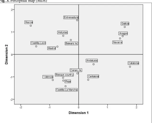
Finally, we analyse the rankings through Multidimensional scaling (MDS) in order to group the regions according to both dimensions. MDS is also known as principal coordinates analysis (Torgerson, 1952). See Borg and Groenen (2005) for an overview of MDS, and Marcussen (2014) for a review of the literature regarding the application of MDS to tourism research. Via MDS we generate a two-dimensional projection of the results in a perceptual map, where we position the seventeen regions according to the similarity between them in terms of their time series features and forecasting resuts.
Fig. 3. Perceptual map (MDS)
Both techniques depict a similar positioning of the regions. In both analysis the Basque Country and La Rioja are grouped together. This result could be due to geographical proximity. Aragon and Galicia are also closely positioned. Asturias and the Balearic Islands, which are the regions that display the worse forecast accuracy for most forecast horizons, are also close together. Catalonia and Murcia are grouped apart from most of the rest of the regions.
7. Conclusions
The increasing importance of the tourism industry worldwide is fostering a growing interest in new approaches to tourism modelling and forecasting. As more accurate predictions become crucial for effective management and policy planning at the regional level, AI techniques allow forecasters to refine predictions. With this objective, we evaluate
the interrelations between time series features and the forecast accuracy of tourism demand predictions obtained with several ML methods (GRP, SVR and NN models).
Making use of international tourism demand to all seventeen regions of Spain, we first apply a seasonal-trend decomposition procedure to compute a set of time series features such as the strength of the trend and the strength of the seasonal component. In a second step, we design a multiple-step-ahead forecasting experiment. We obtain substantially different results across regions. Regarding the different techniques, NNs provide better forecasting results than the other statistical learning models based on interpolation. Finally, we combine the descriptive analysis and the forecasting results, synthesising all the information in two components labelled as “seasonality, trend and forecast accuracy”, and “predictability and dispersion”. By projecting these results on perceptual maps we find that while entropy and dispersion show a negative relation with accuracy for all forecast horizons, the effect of other time series features is heavily dependent on the horizon.
This work provides researchers and practitioners with some evidence on the effect that data characteristics may have on the accuracy of tourism predictions, as well as on the appropriateness of ML techniques for tourism forecasting depending on the forecast horizon. A question left for further research is the incorpation of additional data characteristics in the analysis. Finally, extending the analysis to regions of other destinations would allow to test if there are significant differences across countries.
References
Ahmed, N. K, Atiya, A. F, El Gayar, N., & H. El-Shishiny. (2010). An empirical comparison of machine learning models for time series Forecasting. Econometric Reviews, 29(4), 594–621. Akin, M. (2015). A novel approach to model selection in tourism demand modeling. Tourism
Management, 48, 64–72.
Andrawis, R. R., Atiya, A. F., & El-Shishiny, H. (2011). Forecast combinations of computational intelligence and linear models for the NN5 time series forecasting competition. International
Journal of Forecasting, 27(2), 672–688.
Assaf, A. G., C. P. Barros, & Gil-Alana, L. A.. (2011). Persistence in the short- and long-term tourist arrivals to Australia. Journal of Travel Research, 50(2), 213–229.
Banerjee, S., Gelfand, A. E., Finley, A. O, & Sang, H. (2008). Gaussian predictive process models for large spatial data sets. Journal of the Royal Statistical Society: Series B (Statistical
Methodology), 70, 825–848.
Bardolet, E., & Sheldon, P. J. (2008). Tourism in Archipelagos. Hawai’i and the Balearics.
Annals of Tourism Research, 35(4), 900–923.
Ben Taieb, S., Sorjamaa, A., & Bontempi, G. (2010). Multiple-output modeling for multi-step-ahead time series forecasting. Neurocomputing, 73(10–12), 1950–1957.
Bergmeir, C., Hyndman, R. J., & Benítez, J. M. (2016). Bagging exponential smoothing methods using STL decomposition and Box–Cox transformation. International Journal of
Bilen, M., Yilanci, V., & Eryüzlü, M. (2017). Tourism development and economic growth: a panel Granger causality analysis in the frequency domain. Current Issues in Tourism, 20(1), 27–32.
Borg, I., & Groenen, P. J. F. (2005). Modern multidimensional scaling: Theory and applications (2nd Ed.). New York: Springer-Verlag.
Brida, J. G., Cortés-Jiménez, I., & Pulina, M. (2016). Has the tourism-led growth hypothesis been validated? A literature review. Current Issues in Tourism, 19(5), 394–430.
Broomhead, D. S., & Lowe, D. (1988). Multi-variable functional interpolation and adaptive networks. Complex Systems, 2(3), 321–355.
Burger C, M. Dohnal, M. Kathrada, & Law, R. (2001). A practitioners guide to time-series methods for tourism demand forecasting: A case study for Durban, South Africa. Tourism
Management, 22(4), 403–409.
Cang, S. (2014). A comparative analysis of three types of tourism demand forecasting models: individual, linear combination and non-linear combination. International Journal of Tourism
Research, 16(6), 596–607.
Chen, K. Y., & Wang, C. H. (2007). Support vector regression with genetic algorithms in forecasting tourism demand. Tourism Management, 28(1), 215–226.
Cho, V. (2003). A comparison of three different approaches to tourist arrival forecasting. Tourism
Management, 24(2), 323–330.
Chou, M. C. (2013). Does tourism development promote economic growth in transition countries? A panel data analysis. Economic Modelling, 33, 226–232.
Chu, F. L. (2009). Forecasting tourism demand with ARMA-based methods. Tourism
Management, 30(5), 740–751.
Claveria, O. (2016). Positioning emerging tourism markets using tourism and economic indicators. Journal of Hospitality and Tourism Management, 29, 143–153.
Claveria, O., & Torra, S. (2014). Forecasting tourism demand to Catalonia: Neural networks vs. time series models. Economic Modelling, 36, 220–228.
Claveria, O., E. Monte, & Torra, S. (2015). A new forecasting approach for the hospitality
industry. International Journal of Contemporary Hospitality Management, 27(6), 1520–1538. Claveria, O., Monte, E., & Torra, S. (2016a). Combination forecasts of tourism demand with
machine learning models. Applied Economics Letters, 23 (6), 428–431.
Claveria, O., Monte, E., & Torra, S. (2016b). Modelling cross-dependencies between Spain’s regional tourism markets with an extension of the Gaussian process regression model. SERIEs, 7(3), 341–357.
Claveria, O., Monte, E., & Torra, S. (2017a). Data pre-processing for neural networks-based forecasting: Does it really matter? Technological and Economic Development of Economy, 23(5), 709–725.
Claveria, O., Monte, E., & Torra, S. (2017b). The appraisal of machine learning techniques for tourism demand forecasting. In Roger Inge and Jan Leif (Eds.), Machine Learning: Advances
in Research and Applications. Hauppauge NY: Nova Science Publishers. Chapter 2, 59–90.
Cleveland, W. S. (1979). Robust locally weighted regression and smoothing scatterplots. Journal of the American Statistical Association, 74(368), 829–836.
Cleveland, R. B., Cleveland, W. S., McRae, J. E., & Terpenning, I. (1990). Stl: A seasonal-trend decomposition procedure based on loess. Journal of Official Statistics, 6(1), 3–73.
Cortes, C., & Vapnik, V. (1995). Support-vector networks. Machine Learning, 20(3), 273–297. Cortés-Jiménez, I., & Blake, A. (2011). Tourism demand modeling by purpose of visit and
nationality. Journal of Travel Research, 50(4), 4408–416.
Cristianini, N., & Shawhe-Taylor, J. (2000). An introduction to support vector machines and
other kernel-based learning methods. Cambridge: Cambridge University Press.
Çuhadar, M., I. Cogurcu, & Kukrer, C. (2014). Modelling and forecasting cruise tourism demand to İzmir by different artificial neural network architectures. International Journal of Business
and Social Research, 4(3), 12–28.
Drucker, H., Burges, C. J. C., Kaufman, L., Smola, A., & Vapnik, V. (1997). Support vector regression machines. In M. Mozer, M. Jordan, and T. Petsche (Eds.), Advances in Neural
Gounopoulos, D., Petmezas, D., & Santamaria, D. (2012). Forecasting tourist arrivals in Greece and the impact of macroeconomic shocks from the countries of tourists’ origin. Annals of
Tourism Research, 39(2), 641–666.
Guizzardi, A., & Stacchini, A. (2015). Real-time forecasting regional tourism with business sentiment surveys. Tourism Management, 47, 213–223.
Gunter, U., & Önder, I. (2015). Forecasting international city tourism demand for Paris: Accuracy of uni- and multivariate models employing monthly data. Tourism Management, 46, 123– 135.
Hair, J. F., Black, W. C., Babin, B. J., & Anderson, R. E. (2009). Multivariate data analysis (7th Ed.). Upper Saddle River, NJ: Prentice Hall.
Hassani, H., Silva, E. S., Antonakakis, N., Filis, G., & Gupta, R. (2017). Forecasting accuracy evaluation of tourist arrivals. Annals of Tourism Research, 63, 112–127.
Hassani, H., Webster, A., Silva, H., E. M., & Heravi, S. (2015). Forecasting U.S. tourist arrivals using optimal singular spectrum analysis. Tourism Management, 46, 322–335.
Hong, W. C. (2006). The application of support vector machines to forecast tourist arrivals in Barbados: An empirical study. International Journal of Management, 23(2), 375–385. Hong, W., Dong, Y., Chen, L., & Wei, S. (2011). SVR with hybrid chaotic genetic algorithms for
tourism demand forecasting. Applied Soft Computing, 11(1), 1881–1890.
Hyndman, R. J., Kang, Y., & Smith-Miles, K. (2016). Exploring time series collections used for forecast evaluation. Proceedigns of the 36th International Symposium on Forecasting. Santander, Spain.
Jolliffe, I. T. (2002). Principal component analysis (2nd Ed.). Springer Series in Statistics. Kim, D., & Shwartz, Y. (2013). The accuracy of tourism forecasting and data characteristics: a
meta-analytical approach. Journal of Hospitality Marketing and Management, 22(4), 349– 374.
Kon, S., & Turner, L. L. (2005). Neural network forecasting of tourism demand. Tourism
Economics, 11(3), 301–328.
Krige, D. G. (1951). A statistical approach to some basic mine valuation problems on the Witwatersrand. Journal of the Chemistry, Metallurgical and Mining Society of South Africa, 52(6), 119–139.
Law, R. (2000). Back-propagation learning in improving the accuracy of neural network-based tourism demand forecasting. Tourism Management, 21(3), 331–340.
Lehmann, R., & Wohlrabe, K. (2013). Forecasting GDP at the regional level with many predictors. German Economic Review, 16(2), 226–254.
Li, G., Song, H., Cao, Z., & Wu, D. C. (2013). How competitive is Hong Kong against its competitors? An econometric study. Tourism Management, 36, 247–256.
Li, G., Song, H., & Witt, S. (2005). Recent developments in econometric modeling and forecasting. Journal of Travel Research, 44(1), 82–99.
Lin, C., Chen, H., & Lee, T. (2011). Forecasting tourism demand using time series, artificial neural networks and multivariate adaptive regression splines: Evidence from Taiwan.
International Journal of Business Administration, 2(1), 14–24.
Lin, S., Liu, A., & Song, H. (2015). Modeling and forecasting Chinese outbound tourism: An econometric approach. Journal of Travel & Tourism Marketing, 32(1-2), 34–49.
Linting, M., Meulman, J. J., Groenen, P. J. F., & Van der Kooij, A. J. (2007). Nonlinear principal component analysis: Introduction and application. Psychological Methods, 12(3), 336–358. MacKay, D. J. C. (2003). Information theory, inference, and learning algorithms. Cambridge:
Cambridge University Press.
Marcussen, C. H. (2014). Multidimensional scaling in tourism literature. Tourism Management
Perspectives, 12, 31–40.
Matheron, G. (1973). The intrinsic random functions and their applications. Advances in Applied
Probability, 5(2), 439–468.
Medeiros, M. C., McAleer, M., Slottje, D., Ramos, V., & Rey-Maquieira, J. (2008). An alternative approach to estimating demand: Neural network regression with conditional volatility for high frequency air passenger arrivals. Journal of Econometrics, 147(1), 372– 383.
Molinet, T., Molinet, J. A., Betancourt, M. E., Palmer, A., & Montaño, J. J. (2015). Models of artificial neural networks applied to demand forecasting in nonconsolidated tourist
destinations. Methodology: European Journal of Research Methods for the Behavioral and
Social Sciences, 11(2), 35–44.
Padhi, S. S., & Aggarwal, V. (2011). Competitive revenue management for fixing quota and price of hotel commodities under uncertainty. International Journal of Hospitality Management, 30(3), 725–734.
Pai, P. F., & Hong, W. C. (2005). An improved neural network model in forecasting arrivals.
Annals of Tourism Research, 32(4), 1138–1141.
Palmer, A., Montaño, J. J., & A. Sesé. 2006. Designing an artificial neural network for forecasting tourism time-series. Tourism Management, 27(4), 781–790.
Pattie, D. C., & Snyder, J. (1996). Using a neural network to forecast visitor behavior. Annals of
Tourism Research, 23(1), 151–164.
Peng, B., H. Song, & Crouch, G. I. (2014). A meta-analysis of international tourism demand forecasting and implications for practice. Tourism Management, 45, 181–193.
Quiñonero-Candela, J., & Rasmussen, C. E. (2005). A unifying view of sparse approximate Gaussian process regression. Journal of Machine Learning Research, 6(Dec), 1939–1959. Rasmussen. C. E., & Williams, C. K. I. (2006). Gaussian processes for machine learning.
Cambridge, MA: The MIT Press.
Ripley, B. D. (1996). Pattern recognition and neural networks. Cambridge: Cambridge University Press.
Rosselló, J., & Sansó, A. (2017). Yearly, monthly and weekly seasonality of tourism demand: A decomposition analysis. Tourism Management, 60, 379–389.
Schölkopf, B., & Smola, A. J. (2002). Learning with kernels: Support vector machines,
regularization, optimization, and beyond (Adaptive computation and machine learning
series). Cambridge, MA: MIT Press.
Smola, A. J., & Bartlett, P. L. (2001). Sparse greedy Gaussian process regression. In T. K. Leen, T. G. Dietterich, and V. Tresp (Eds.) Advances in Neural Information Processing Systems, 13 (619-625). Cambridge, MA: The MIT Press.
Song, H., & Li, G. (2008). Tourism demand modelling and forecasting – A review of recent research. Tourism Management, 29(2), 203–220.
Soukiazis, E., & Proença, S. (2008). Tourism as an alternative source of regional growth in Portugal: a panel data analysis at NUTS II and III levels. Portuguese Economic Journal, 7(1), 43–61.
Spearman, C. (1904). The proof and measurement of association between two things. American
Journal of Psychology, 15(1), 72–101.
Tang, C. F., & Abosedra, S. (2016). Tourism and growth in Lebanon: new evidence from
bootstrap simulation and rolling causality approaches. Empirical Economics, 50(2), 679–696. Teixeira, J. P., & Fernandes, P. O. (2012). Tourism time series forecast – Different ANN
architectures with time index input. Procedia Technology, 5, 445–454.
Teräsvirta, T., van Dijk, D., & Medeiros, M. C. (2005). Linear models, smooth transition autoregressions, and neural networks for forecasting macroeconomic time series: A re-examination. International Journal of Forecasting, 21(3), 755–774.
Torgerson, W. S. (1952). Multidimensional scaling: I. Theory and method. Psychometrika, 17(4), 401–419.
Tsaur, R., & Kuo, T. (2011). The adaptive fuzzy time series model with an application to Taiwan’s tourism demand. Expert Systems with Applications, 38(8), 9164–9171.
Tsaur, S., Chiu, Y., & Huang, C. (2002). Determinants of guest loyalty to international tourist hotels: A neural network approach. Tourism Management, 23(4), 397–405.
Tsui, W. H. K., Ozer-Balli, H., Gilbey, A., & Gow, H. (2014). Forecasting of Hong Kong airport’s passenger throughput. Tourism Management, 42, 62–76.
Uysal, M., & El Roubi, M. S. (1999). Artificial neural networks versus multiple regression in tourism demand analysis. Journal of Travel Research, 38(2), 111–118.
Vapnik, V. N. (1995). The nature of statistical learning. New York: Springer-Verlag. Vapnik, V. N. (1998). Statistical learning theory. New York: Wiley.
Williams, C. K. I., & Rasmussen, C. E. (1996). Gaussian processes for regression. Advances in
Neural Information Processing Systems, 8, 514–520.
Witt, S., & Witt. C. (1995). Forecasting tourism demand: A review of empirical research.
International Journal of Forecasting, 11(3), 447–475.
Wu, Q., Law, R., & Xu, X. (2012). A spare Gaussian process regression model for tourism demand forecasting in Hong Kong. Expert Systems with Applications, 39(4), 4769–4774. Xu, X., Law, R., & Wu, T. (2009). Support vector machines with manifold learning and
probabilistic space projection for tourist expenditure analysis. International Journal of
Computational Intelligence Systems, 2(1), 17–26.
Xu, X., Law, R., Chen, W., & Tang, L. (2016). Forecasting tourism demand by extracting fuzzy Takagi–Sugeno rules from trained SVMs. CAAI Transactions on Intelligent Technology, 1, 30–42.
Yu, G., & Schwartz, Z. (2006). Forecasting short time-series tourism demand with artificial intelligence models. Journal of Travel Research, 45(2), 194–203.
Zhang, G., Putuwo, B. E., & Hu, M. Y. (1998). Forecasting with artificial neural networks: the state of the art. International Journal of Forecasting, 14(1), 35–62.
Zhang, C., & Zhang, J. (2014). Analysing Chinese citi The relationship between tourism, foreign direct investment and economic growth: evidence from Iran' intentions of outbound travel: a machine learning approach. Current Issues in Tourism, 17(7), 592–609.
Institut de Recerca en Economia Aplicada Regional i Pública Document de Treball 2014/17, pàg. 5