UNIVERSITY
OF TRENTO
DIPARTIMENTO DI INGEGNERIA E SCIENZA DELL’INFORMAZIONE
38050 Povo – Trento (Italy), Via Sommarive 14
http://www.disi.unitn.it
NOISE REDUCTION FOR INSTANCE-BASED LEARNING
WITH A LOCAL MAXIMAL MARGIN APPROACH
Nicola Segata, Enrico Blanzieri, Sarah Jane Delany
and Padraig Cunningham
October 2008
Noise Reduction for Instance-Based Learning
with a Local Maximal Margin Approach
Nicola Segata
1, Enrico Blanzieri
1, Sarah Jane Delany
2, and P´adraig Cunningham
31
University of Trento (DISI), Italy. {segata,blanzier}@disi.unitn.it
2Dublin Institute of Technology, Ireland. [email protected]
3
University College Dublin, Ireland. [email protected]
October 7, 2008
Abstract
To some extent the problem of noise reduction in machine learning has been finessed by the devel-opment of learning techniques that are noise-tolerant. However, it is difficult to make instance-based learning noise tolerant and noise reduction still plays an important role in k-nearest neighbour classifi-cation. There are also other motivations for noise reduction, for instance the elimination of noise may result in simpler models or data cleansing may be an end in itself.
In this paper we present a novel approach to noise reduction based on local Support Vector Ma-chines (LSVM) which brings the benefits of maximal margin classifiers to bear on noise reduction. This provides a more robust alternative to the majority rule on which almost all the existing noise reduction techniques are based. Roughly speaking, for each training sample an SVM is trained on its neighbour-hood and if the SVM classification for the central sample disagrees with its actual class there is evidence in favour of removing it from the training set. We provide an empirical evaluation on 15 real datasets showing improved classification accuracy when using training data edited with our method as well as specific experiments regarding the spam filtering application domain. We present a further evaluation on two artificial datasets where we analyse two different types of noise (Gaussian sample noise and mislabelling noise) and the influence of different class densities. The conclusion is that LSVM noise reduction is significatively better than the other analysed algorithms for real datasets and for artificial datasets perturbed by Gaussian noise and in presence of uneven class densities.
1 Introduction
The problem of noise in machine learning has been addressed more by developing algorithms that are noise tolerant than by explicitly removing noise. Nevertheless there are a number of circumstances where explicitly removing noise can have merit. It is difficult to make instance-based learning algorithms such as k-nearest neighbour (k-NN) classifiers or case-based reasoning (CBR) noise tolerant so noise reduction can be important for improving generalisation accuracy in instance-based learning. A further motivation for noise reduction in CBR is explanation – a capability that is perceived to be one of the advantages of CBR (Leake, 1996; Cunningham et al, 2003). Since case-based explanation will invoke individual cases as part of the explanation process it is important that noisy cases can be eliminated if possible. Even if noise reduction will not improve the classification accuracy of learning algorithms that have been developed to be noise tolerant, researchers have argued that noise reduction as a preprocessing step can simplify resulting models, an objective that is desirable in many circumstances (Lorena and Carvalho, 2004).
Generally speaking, the random (i.e. not systematic) noise affecting machine learning datasets is mainly of two types: attribute (or feature) noise and class (or mislabelling) noise. The first is almost inevitably present in the data because of errors and approximations on observing and measuring the attributes of the examples. The latter is due to errors in the process of assigning labels to the samples. Moreover other
sources of generalization accuracy problems that cannot be strictly considered noise are outlier samples (i.e. correct samples representing some atypical examples) and contradictory samples (i.e. samples with the same attribute values but different labels). A noise reduction algorithm must deal contemporaneously with all these issues in order to be successfully applied for real problems.
In k-NN and CBR the problem of noise reduction has traditionally been considered part of the larger problem of case-base maintenance. Since large training sets can influence the response time of lazy learners an extensive literature is dedicated to the development of data reduction techniques that preserve training set competence (see Section 3). While the problem of noise in k-NN can be mitigated by increasing the neighbourhood size and using a majority decision rule there has also been a lot of research on compe-tence enhancing techniques that preprocess the training data to remove noisy instances. Such compecompe-tence enhancing techniques are the subject of this work.
We present a novel technique for competence enhancing in the context of k-NN-based classifiers. The approach is based on Local Support Vector Machines (LSVM) (Blanzieri and Melgani, 2006, 2008), a modification of (non linear) Support Vector Machines (SVM) (Cortes and Vapnik, 1995) that takes locality into account. By extending LSVM with a probabilistic output we apply it on the training set to remove noisy, corrupted and mislabelled samples. This is done by building a local model in the neighbourhood of each training sample and the sample is removed if the probability associated with the correct classification is below a threshold. In other words we remove those samples that, with respect to the maximal separating hyperplanes built on the feature space projections of their neighbourhoods, are too close to or on the wrong side of the decision boundary. From another viewpoint we simply augment the majority rule criterion used by most competence enhanced techniques (see section 3.2) with the kernel-space maximal margin principle.
In the evaluation we present in this paper we compare the performance of our LSVM-based strategy against three state-of-the-art noise reduction techniques from the literature (see section 3.2). The LSVM strategy comes out on top against these techniques on a range of 15 real world datasets and on six spam filtering datasets. It also performs very well on artificial datasets where we consider feature noise, label noise and unbalanced class distributions.
The paper is organized as follows. In the next section we elaborate on the motivations for noise re-duction before we review the literature on training set editing in section 3. In section 4 we introduce our method that is empirical evaluated in section 5 on a number of real and artificial datasets. The paper closes with conclusions and some reflections on promising directions for future work.
2 Motivation
There are a number of reasons for performing noise reduction on training datasets in instance based learn-ing. The primary one being that instance based techniques have a dependency on individual training sam-ples that other supervised learning techniques do not have. Other techniques have been developed to be noise tolerant by incorporating into the induction process mechanisms that attempt to avoid overfitting to noise in the training set. Examples of this include early stopping for artificial neural networks (Cataltepe et al, 1999), the post-pruning of decision trees (Quinlan, 1986) and using soft-margin Support Vector Ma-chines which relax the constraints on the margin maximisation (Vapnik, 1999). However, instance based techniques such as k-NN that rely on specific retrieved instances for induction are affected by noise. These techniques generally lack the induction step that other noise tolerant techniques can adapt. The dependance on the specific retrieved instances can be reduced by retrieving more instances (i.e. k-NN, with k > 1 is more noise tolerant than 1-NN) but accuracy will not always increase with larger values of k. At some point a large k will result in a neighbourhood that crosses the decision surface and accuracy will drop.
An additional motivation for noise reduction in instance based learning associated with this dependency on individual training samples is case-based explanation. A learning system that can provide good expla-nations for its predictions can increase user confidence and trust and give the user a sense of control over the system (Roth-Berghofer, 2004). Case-based explanations are generally based on a strategy of present-ing similar past examples to support and justify the predictions made (Cunnpresent-ingham et al, 2003; Nugent et al, 2008). If specific cases are to be invoked as explanations then noisy cases need to be identified and removed from the case-base.
Finally there are specific application areas where noise reduction is important. It is generally accepted that inductive learning systems in the medical domain are dependent on the quality of the data (Pechenizkiy et al, 2006) and there has been significant research into data cleansing in bioinformatics (Malossini et al, 2006; Gamberger et al, 2000; Lorena and Carvalho, 2004; Tang and Chen, 2008a,b). Although instance based techniques such as k-NN are not generally used for classification in much of this research, noise reduction is an important element in the process as it can result in the simplification of the models created. Lorena and Carvalho (2004), for example, found that preprocessing the training data to remove noise resulted in simplifications in induced SVM classifiers and higher comprehensiveness in induced decision tree classifiers.
3 Review of editing techniques
Editing strategies for IBL and CBR can have many different objectives as discussed, for example, by Wilson and Martinez (2000) and Brighton and Mellish (2002). According to them, editing techniques can be categorised as competence preservation or competence enhancement techniques. Competence preservation techniques aim to reduce the size of the training set as much as possible without significantly affecting the generalisation accuracy thus achieving a reduction in the storage requirements and increasing the speed of execution. The main goal of competence enhancement techniques is to increase the generalisation accuracy primarily by removing noisy or corrupt training examples.
Obviously, some strategies aim to tackle both objectives at the same time and for this reason are called hybrid techniques (Brighton and Mellish, 2002). Although the technique we introduce in this work can theoretically be considered a hybrid technique, we will focus our evaluation on competence enhancement. For this reason in the following discussion of editing methods, we focus on existing techniques that demon-strate good generalisation accuracy.
Editing strategies normally operate in one of two ways; incremental which involves adding selected examples from the training set to an initially empty edited set, and decremental which involves contracting the training set by removing selected examples.
3.1 Competence preservation methods
Competence preservation was studied almost simultaneously with the introduction of nearest neighbour classifiers mostly because of the limited power of early computational systems. The first contribution was Hart’s Condensed Nearest Neighbour Rule (CNN) (Hart, 1968) which incrementally populates the edited set with those training examples that are misclassified by the edited set. Improvements over the CNN rule, primarily developed to overcome its limitations in the presence of noise, are the Reduced Nearest Neighbour Rule (RNN) by Gates (1972) and the Selective Nearest Neighbour Rule (SNN) by Ritter et al (1975). RNN is a decremental technique which removes an example from the edited set where its removal does not cause any other training example to be misclassified while SNN imposes the rule that every training example must be closer to an example of the same class in the edited set than to any training example of another class.
CNN (using 1-NN) is included as a special case in the Generalized Condensed Nearest Neighbour Rule (GCNN) (Chou et al, 2006) which relaxes the criterion for correct classification by a factor of the minimum distance between heterogeneous examples in the training set. Another variation on the CNN rule for text categorisation is reported by Hao et al (2008) which orders the training examples for rule consideration based on a metric calculated from the document’s textual feature weights. Recently, the novel Fast Condensed Nearest Neighbor Rule (FCNN) has been introduced by Angiulli (2007). FCNN offers advantages over other CNN variations as it is an order-independent algorithm, it exploits the triangle inequality to reduce computational effort and it is scalable on large multidimensional datasets.
A different approach based on prototypes is proposed by Chang (1974) in which the nearest two training examples belonging to the same class are merged using a weighting policy into a new example. A limitation of this approach is that the new training examples are synthetically constructed eliminating the original examples and this prohibits, for example, case-based explanation.
More recent approaches to case-base editing in the CBR paradigm use the competence properties of the training examples or cases to determine which ones to include in the edited set. Measuring and using case competence to guide case-base maintenance was first introduced by Smyth and Keane (1995) who introduced two important competence properties, the reachability and coverage sets for a case in a case-base. The reachability set of a case t, which is the set of all cases that can correctly classify t and the coverage set which is the set of all examples that t can correctly classify. An example of using case competence to guide editing is the Footprint Deletion policy by Smyth and Keane (1995) which is based on the notion of a competence footprint, a subset of training examples providing the same competence as the entire set. The same group also proposes a family of competence-guided methods (McKenna and Smyth, 2000) based on different combinations of four features; an ordering policy, an addition rule, a deletion rule and a competence update policy. Brighton and Mellish (2002) also used the competence properties of cases in their Iterative Case Filtering (ICF) algorithm which is a decremental algorithm that contracts the training set by removing those cases c, where the number of other cases that can correctly classify c is higher that the number of cases that c can correctly classify. Most competence-based editing techniques can include a preprocessing step for noise removal thus becoming hybrid methods.
Salam´o and Golobardes (2001) propose techniques based on the theory of Rough Sets (Pawlak, 1991) which reduce the case-base by analysing the lower and upper approximations to sets of training instances that are indistinguishable with regard to a specific subset of features. Successive refinements from the same authors incorporate their rough sets measures into Smyth and Keane (1995)’s competence model and then apply various policies for removing cases (Salam´o and Golobardes, 2002, 2004). Similar approaches have been proposed by Cabailero et al (2005) who creates the edited training data from the lower and upper set approximations and Cao et al (2001) who couples rough sets theory with fuzzy decision tree induction.
Mitra et al (2002) present an incremental density-based approach to editing large datasets which uses a nearest neighbour density estimate of the underlying training data to select which examples to keep. The density based approach is further developed by Huang and Chow (2005) introducing the concept of entropy while a successful application of density-based reduction for text categorization is detailed in (Li and Hu, 2003).
3.2 Competence enhancement methods
The objective of competence enhancement methods is to remove noisy, mislabelled and borderline exam-ples that are likely to cause misclassification thus allowing k-NN classifiers to build smoother decision surfaces. In its pure form, competence enhancement will retain all the correctly labelled samples far from the decision boundary thus precluding significant storage reduction. Competence enhancement techniques start with Wilson’s Edited Nearest Neighbor algorithm (ENN) (Wilson, 1972). It is a decremental strategy that simply removes from the training set those examples that do not agree with the majority of their k nearest neighbours.
Tomek (1976) proposed two improvements to ENN; Repeated Edited Nearest Neighbor (RENN) and All-kNN (AkNN). Both RENN and AkNN make multiple passes over the training set repeating ENN. RENN just repeats the ENN algorithm until no further eliminations can be made from the edited set while AkNN repeats ENN for each sample using incrementing values of k each time and removing the sample if its label is not the predominant one at least for one value of k. It is worth noting that for k = 1, ENN and AkNN are equivalent and for k > 1 AkNN is more aggressive than ENN.
A slightly different approach is introduced by Koplowitz and Brown (1981) which considers the rela-belling of some examples instead of their removal. This idea is expanded on by Jiang and Zhou (2004) who use an ensemble of neural networks to determine the label for the examples that are to be relabelled. Another modification of ENN and RENN proposed by S´anchez et al (2003) entails substituting the k near-est neighbours with the k nearnear-est centroid neighbours (k-NCN) where the neighbourhood of an example is defined not only based on distances from the example but also on the symmetrical distribution of examples around it.
The detecting of mislabeled samples in high-dimensional spaces with small sample size (the typical characteristics of microarray data in bioinformatics) is addressed by Malossini et al (2006) based on a leave-one-out perturbation matrix and a measure of the stability of the label of a sample with respect to label changes of other samples.
In the context of editing training data for spam filtering systems, Delany and Cunningham (2004) advocate putting the emphasis on examples that cause misclassifications rather than the examples that are themselves misclassified. The method which is called Blame Based Noise Reduction (BBNR) enhances the competence properties of coverage and reachability with the concept of a liability set. Roughly speaking this set, which is defined for each training example t in a leave-one-out classification of the training set, contains any other misclassified training examples (of a different class than t) where t contributed to the misclassification by being returned as one of the k nearest neighbours.
3.3 Hybrid methods.
Instance Based (IB) Learning Algorithms (IBn), presented by Aha et al (1991), can be considered the first hybrid approaches to editing. IB2 is an online learning method, similar to CNN, that works by adding to an initially empty set those examples that are not correctly classified by the edited set. Within this setting a newly available example that is not added to the edited set does not need to be stored. On the other hand, since noisy and mislabelled examples are very likely to be misclassified, they are almost always maintained in the edited set. In order to overcome this weakness, IB3 adds a “wait and see” policy which records how well examples are classifying and only keeps those that classify correctly to a statistically signicant degree. Variations of the IBn algorithms are Typical Instance Based Learning algorithm (TIBL) (Zhang, 1992) which tries to keep examples near the centre of clusters rather than on decision boundaries, Model Class Selection techniques (MCS) (Brodley, 1993) which checks the class-consistency of a example with respect to the examples it classifies, and methods based on Encoding Length Heuristic (ELH) (Cameron-Jones, 1995).
Another hybrid method proposed by Lowe (1995) is based on Variable-Kernal Similarity Metric (VSM) Learning. In this case an example is removed if its neighbourhood is classified by the VSM classifier as belonging to the same class. In this way examples internal to clusters are removed but as there is no requirement that the removed example has the same class as its neighbours, this technique also removes ‘noisy’ examples.
Wilson and Martinez (1997) introduced a family of Reduction Techniques (RT1, RT2 and RT3) which were then enhanced by Wilson and Martinez (2000) under the name of Decremental Reduction Optimiza-tion Procedures (DROP1-DROP5) and Decremental Encoding Length (DEL). DROP1 is very similar to RNN with the only difference that the misclassifications are checked in the edited set instead of the train-ing set. DROP2 fixes the order of presentation of examples as those furthest from their nearest unlike neighbour (i.e. nearest example of a different class) to remove examples furthest from the class borders first. DROP2 also uses the original training set when checking for misclassification to avoid some prob-lems that can occur with DROP1 such as removing entire clusters. In order to make DROP2 more robust to noise, DROP3 introduces an explicit noise reduction preprocessing stage with a rule very similar to ENN. In DROP4 this noise reduction phase is made more conservative by only removing an example if it is misclassified by its neighbourhood and if its removal does not hurt the classification of other instances. DROP5 is a modification of DROP2 using the opposite ordering function for the presentation of examples which acts as a noise reduction pass and finally DEL is a version of DROP3 using ELH as the deletion rule. Recently a new case-base mining framework has been introduced by Pan et al (2007). The frame-work includes a case-base mining algorithm which is based on a theoretical foundation. The Kernel-based Greedy Case-base Mining (KGCM) algorithm first maps the examples to a new feature space through a kernel transformation, performs a Fisher Discriminant Analysis (FDA) based feature-extraction method to help remove noise and extract the highly predictive features and finally considers the diversity of the selected cases in terms of the coverage of future problems.
3.4 Benchmarking noise reduction and generalisation accuracy enhancement
The main editing techniques developed before 2000 have been extensively evaluated by Wilson and Mar-tinez (2000). The overall result of their analysis is that DROP3 has the best mix of generalisation accuracy and storage reduction. However, looking at generalisation capability only, they conclude that their DROP3 method has somewhat lower accuracy that the group of methods including ENN, RENN and AkNN. In
particular, among these last three methods, AkNN has “the highest accuracy and lowest storage require-ments in the presence of noise” (Wilson and Martinez, 2000). The comparisons of ICF with DROP3 done by (Brighton and Mellish, 2002) highlights that they have similar performance but, considering the accu-racy results only, it is clear that ENN outperforms both in the majority of the datasets.
k-NCN seems to be more accurate than AkNN and ENN as shown by S´anchez et al (2003), but the analysis is performed on five datasets only and does not include an assessment of statistical significance. Moreover k-NCN substitutes real samples with synthetic ones preventing CBR explanation. Without con-sidering the competence preserving methods as our objective is competence enhancement, the remaining approaches (including the neural network ensemble approach presented by Jiang and Zhou (2004) and KGCM (Pan et al, 2007)) do not provide any comparison with ENN, RENN or AkNN and the reproduction of these techniques is non trivial as they are embedded in complex frameworks. The approach proposed by Malossini et al (2006) is conceived for very high dimensional datasets with very few samples and thus it is not suitable for general real datasets.
Taking this into consideration, we chose to empirically compare our proposed noise reduction technique with AkNN as, despite its simplicity, it still represents the state-of-the-art for competence enhancement. We also include comparisons with RENN as it is the most popular noise reduction technique used in the literature. Moreover we include BBNR in the evaluation because as it has only been applied for the spam filtering task, it is of interest to test its performance in general classification problems.
4 Noise reduction with local support vector machines
Our novel approach for noise reduction for CBR and IBL tasks based on Local SVM is introduced in this section. In a departure from previous work in this area we do not use CBR rules to detect the samples that do not agree with their neighbourhood. Instead, we apply a localized SVM decision function around each training sample and remove it if the predicted probability of the actual class is too low. Notice that we maintain the locality assumption for noise reduction which is present in the traditional editing techniques.
We briefly introduce a formal definition of the k-nearest neighbour classifier and support vector ma-chines before presenting the local version of support vector mama-chines and the associated noise reduction technique.
In the following we assume a classification problem with samples (xi, yi) with i = 1, . . . , n, xi∈ Rpand
yi∈ {+1, −1}. The set of xipoints belonging to the training set is denoted with X.
4.1 k-nearest neighbour classifier
We formally define the k-NN method here because we will use the notation in the description of the local support vector machine method. Given a point x0, it is possible to order the entire set of training samples
X with respect to x0. This corresponds to defining a function rx0 : {1, . . . , n} → {1, . . . , n} that recursively
reorders the indexes of the n training points: rx0(1) = argmin i=1,...,n kxi− x0k rx0( j) = argmin i=1,...,nkxi− x 0k i 6= r x0(1), . . . , rx0( j − 1) for j = 2, . . . , n
In this way, xrx0( j)is the point of the set X in the j-th position in terms of distance from x0, namely the
j-th nearest neighbour, kxrx0( j)− x0k is its distance from x0and yrx0( j)is its class with yrx0( j)∈ {+1, −1}. In
other terms: j < k ⇒ kxrx0( j)− x 0k ≤ kx
rx0(k)− x 0k.
Given the above definition, the majority decision rule of k-NN for binary classification problems is defined by kNN(x) = sign à k
∑
i=1 yrx(i) ! .4.2 Support vector machines
SVMs (Cortes and Vapnik, 1995) are classifiers with sound foundations in statistical learning theory (Vap-nik, 1999). The decision rule is SV M(x) = sign(hw, Φ(x)iF+ b) where Φ(x) : Rp→ F is a mapping in
a transformed feature space F with inner product h·, ·iF. The parameters w ∈ F and b ∈ R are such
that they minimize an upper bound on the expected risk while minimizing the empirical risk. The mini-mization of the complexity term is achieved by minimizing the quantity 12· kwk2, which is equivalent to maximizing the margin between the classes. The empirical risk term is controlled through the following set of constraints:
yi(hw, Φ(xi)iF+ b) ≥ 1 −ξi ξi≥ 0, i = 1, . . . , n (1)
where yi∈ {+1, −1} is the class label of the i-th nearest training sample. The presence of the slack
variablesξiallows some misclassification on the training set. Reformulating such an optimization problem
with Lagrange multipliersαi(i = 1, . . . , n), and introducing a positive definite kernel (PD) function1K(·, ·)
that substitutes the scalar product in the feature space hΦ(xi), Φ(x)iF the decision rule can be expressed
as: SV M(x) = sign à n
∑
i=1 αiyiK(xi, x) + b ! .The kernel trick avoids the explicit definition of the feature space F and of the mapping Φ (Schlkopf and Smola, 2001). Popular kernels are the linear (LIN) kernel, the radial basis function (RBF) kernel, and the homogeneous (HPOL) and inhomogeneous (IPOL) polynomial kernels. Their definition are:
klin(x, x0) = hx, x0i krb f(x, x0) = expkx−x0k2
σ
khpol(x, x0) = hx, x0id kipol(x, x0) = (hx, x0i + 1)d.
The maximal separating hyperplane defined by SVM has been shown to have important generalisation properties and nice bounds on the VC dimension (Vapnik, 1999).
In their original formulation, SVMs are not able to give probability estimates for query samples. In order to obtain the probability estimate that a sample xihas positive class label, i.e. bpSV M(y = +1|x) =
1 − bpSV M(y = −1|x) , Platt (1999b) proposed the following approximation refined by Lin et al (2007):
b
pSV M(y = +1|x) = 1
1 + exp(A · SV M(x) + B)
where A and B are parameters that can be estimated by minimizing the negative log-likelihood using the training set and the associated decision values (using for example cross validation).
4.3 Local support vector machine
The method (Blanzieri and Melgani, 2006, 2008) combines locality and search for a large margin sepa-rating surface by partitioning the entire transformed feature space through a set of local maximal margin hyperplanes. It can be seen as a modification of the SVM approach in order to obtain a local learning algorithm (Bottou and Vapnik, 1992) able to locally adjust the capacity of the training systems. The lo-cal learning approach is particularly effective for uneven distributions of training set samples in the input space. Although k-NN is the simplest local learning algorithm, its decision rule based on majority voting overlooks the geometric configuration of the neighbourhood. For this reason the adoption of a maximal margin principle for neighbourhood partitioning can result in a good compromise between capacity and number of training samples (Vapnik, 1991).
In order to classify a given point x0of the input space, we need first to find its k nearest neighbours in
the transformed feature space F and, then, to search for an optimal separating hyperplane only over these k nearest neighbours. In practice, this means that an SVM is built over the neighbourhood of each test point x0. Accordingly, the constraints in (1) become:
yrx(i)¡w · Φ(xrx(i)) + b¢≥ 1 −ξrx(i), with i = 1, . . . , k
1For convention we refer to kernel functions with the capital letter K and to the number of nearest neighbours with the lower-case
where rx0: {1, . . . , n} → {1, . . . , n} is a function that reorders the indexes of the training points defined as: rx0(1) = argmin i=1,...,nkΦ(xi) − Φ(x 0)k2 rx0( j) = argmin i=1,...,nkΦ(xi) − Φ(x 0)k2 i 6= r x0(1), . . . , rx0( j − 1) for j = 2, . . . , n
In this way, xrx0( j)is the point of the set X in the j-th position in terms of distance from x
0and the thus
j < k ⇒ kΦ(xrx0( j)) − Φ(x0)k ≤ kΦ(x
rx0(k)) − Φ(x
0)k because of the monotonicity of the quadratic operator.
The computation is expressed in terms of kernels as: ||Φ(x) − Φ(x0)||2=
= hΦ(x), Φ(x)iF+ hΦ(x0), Φ(x0)iF− 2 · hΦ(x), Φ(x0)iF=
= K(x, x) + K(x0, x0) − 2 · K(x, x0). (2)
If the kernel is the RBF kernel or any polynomial kernels with degree 1, the ordering function is equivalent to using the Euclidean metric. For some non-linear kernels (other than the RBF kernel) the ordering function can be quite different to that produced using the Euclidean metric.
The decision rule associated with the method is: kNNSVM(x) = sign
Ã
k
∑
i=1
αrx(i)yrx(i)K(xrx(i), x) + b !
. (3)
For k = n, the k-NNSVM method is the usual SVM whereas, for k = 2, the method implemented with the LIN or RBF kernel corresponds to the standard 1-NN classifier. Notice that in situations where the neighbourhood contains only one class the local SVM does not find any separation and so considers all the neighbourhood to belong to the predominant class thus simulating the behaviour of the majority rule.
Considering k-NNSVM as a local SVM classifier built in the feature space, the method has been shown to potentially have a favourable bound on the expectation of the probability of test error with respect to SVM (Blanzieri and Melgani, 2008).
The probability output for this method can be obtained using the local SVM probability estimation as follows:
b
pkNNSV M(y = +1|x) = 1
1 + exp(A · kNNSV M(x) + B)
This local learning algorithm based on SVM has been successfully applied for remote sensing tasks by (Blanzieri and Melgani, 2006) and on 13 benchmark datasets (Segata and Blanzieri, 2008), confirm-ing the potential of this approach.
4.4 Local support vector machine for noise reduction
Local learning algorithms can be applied in the training set with a leave-one-out strategy to detect the samples that would not be correctly predicted by their neighbourhood. The noise reduction techniques for CBR proposed in in the literature so far use strategies in the spirit of case-based local learning. Here, using the LSVM approach, we can apply the maximal margin principle to the neighbourhood of each training sample to verify if the actual label of the central point is correctly predicted. What is theoretically appealing about LSVM for noise removal, is its compromise between the discrimination ability of SVM with respect to the majority voting and the local application of the maximal margin principle which is crucial since the final classification is performed with an inherently local nearest neighbour strategy.
The set X0⊆ X of training samples without the noisy samples detected by kNNSVM is thus defined,
using Equation 3, as follows:
X0=©xi∈ X
¯
¯ kNNSVM(xi) = yi
ª .
Although LSVM is a local learning algorithm, its decision rule (the maximal margin separation) can be very different from the k-NN decision rule (majority rule) which will be used in the final classifier. For this reason and, more generally, in order to be able to adapt to different types and levels of noise, it is desirable
to have the possibility to tune the aggressiveness of the removing policy. This can be achieved using the probabilistic output of LSVM as follows:
X0= n xi∈ X ¯ ¯ bpkNNSV M(y = y i|xi) >γ o .
Theγthreshold can be manually tuned to modify the amount of noise to be removed and the probability level associated with non-noisy samples. Intuitively, we expect that for very low values of bpkNNSV M(y =
yi|xi), xi corresponds to a mislabelled sample, while for values near 0.5, xi could be a noisy sample or a
sample close to the decision surface. High values ofγ can be used to maintain in the training set only samples for which kNNSVM is highly confident in their labels, theoretically enhancing the separation between the classes. The locality of the approach is regulated by the k parameter and can be enhanced by using a local kernel such as the RBF kernel (Genton, 2001) or by applying a quasi-local kernel operator to a generic kernel as described in (Segata and Blanzieri, 2007).
Although not empirically tested and discussed in this work, the same framework can be used to perform competence preservation (or redundancy reduction) by simply changing the comparison operator:
X0=nx i∈ X ¯ ¯ bpkNNSV M(y = y i|xi) <γ o .
The idea, in this case, is to remove the samples that are very likely to be correctly classified maintaining in the training set only the samples that are close to decision boundary. A further quite straightforward modification would allow the integration of competence preservation and competence enhancement:
X0=nx i∈ X ¯ ¯γ0< bpkNNSV M(y = y i|xi) <γ00 o .
5 Evaluation
As stated in section 3.4 the alternative noise reduction strategies we choose to benchmark against our local SVM strategy are RENN, AkNN and BBNR (see section 3 for details). Although multiple evaluation strategies for editing techniques for IBL and CBR can be considered (Wilson and Martinez, 2000), we focus here on analysing the change in generalisation accuracy which is arguably the more important aspect in a noise reduction context. However, for completeness, we also present figures for the reduction in the training set for each technique.
The model selection is performed as follows. For RENN, AkNN and BBNR the k parameter is chosen as the one giving the best k-NN 20-fold cross validation accuracy. Preliminary results indicated that this choice permits much more accuracy gain with the edited training set compared with the alternative of fixing k to 1 or 3 as usually done in literature. For LSVM noise reduction we use the RBF kernel and, as with the other techniques, we select the value of k and the other parameters (the regularization parameter C and the kernel widthσ) giving the best 20-fold cross classification accuracy of the associated LSVM classifier. To select the noise thresholdγfor LSVM we perform 20-fold cross validation editing on the training set. The generalisation accuracy reported are results on the test set using 1-NN or 3-NN classifiers. If a separated test set is not available we randomly remove 1/4 of the training set samples and use them for testing.
The LSVM noise reduction and the associated LSVM classifier (used for model selection) are imple-mented using the LibSVM library (Chang and Lin, 2001) for training and evaluating the local SVM models. We implemented also RENN and AkNN, while for BBNR we used the jColibr`ı 2.0 framework (Bello-Tom´as et al, 2004; D´ıaz-Agudo et al, 2007).
5.1 Evaluation on 15 real datasets
We consider 15 binary-class datasets with no more than 5000 samples and no more than 300 features from the UCI repository (Asuncion and Newman, 2007) and the LibSVM website (Chang and Lin, 2001). The datasets have only numerical feature values and are scaled to the [0, 1] interval. The characteristics of the 15 datasets are reported in Table 1.
3Currently the evaluation of BBNR on theA3AandW1Adatasets is not yet terminated. However, we expect that the overall
dataset brief description source training set testing set number of name cardinality cardinality features
A3A Adult dataset preprocessed as done by Platt (1999a) LibSVM 3185 29376 123
ASTRO astroparticle application from Uppsala University UCI 3089 4000 4
AUSTRALIAN australian credit approval, originally from Statlog LibSVM 517 173 14
BREAST Wisconsin breast cancer data UCI 512 171 10
CMC contraceptive method choice data UCI 1104 369 8
DIABETES Pima indians diabetes data LibSVM 576 192 8
LETTER MN Statlog letter recognition data (M and N only) LibSVM 1212 363 16
MAM mammographic cancer screening mass data UCI 720 241 5
MUSK2 musks/non-musks molecule prediction, version 2 UCI 4948 1650 166
NUMER German numeric credit risk, originally from Statlog LibSVM 750 250 24
DIGIT06 handwritten digits recognition (0 and 6 only) UCI 1500 699 16
DIGIT12 handwritten digits recognition (1 and 2 only) UCI 1559 728 16
SPAMBASE spam filtering data UCI 3450 1151 57
SPLICE primate splice-junction gene sequences data LibSVM 1000 2175 60
W1A web page classification, originally from Platt (1999a) LibSVM 2477 47272 300
Table 1: The 15 datasets used in the experiments of Section 5.1. dataset 1-NN test set accuracy training set reduction
uned. RENN AkNN BBNR LSVM RENN AkNN BBNR LSVM
A3A 78.23 81.94 82.66 82.62 19.9% 34.1% 30.7% ASTRO 93.93 94.75 95.03 92.28 94.98 4.5% 6.1% 8.8% 2.5% AUSTRALIAN 82.66 84.97 84.39 64.74 84.97 14.3% 27.9% 63.4% 72.5% BREAST 82.08 90.17 90.17 83.23 89.02 16.2% 32.7% 21.1% 11.0% CMC 53.39 60.70 57.99 53.39 63.14 38.5% 50.0% 22.1% 26.0% DIABETES 66.67 66.15 67.19 58.33 70.31 31.3% 41.0% 40.6% 28.8% LETTER MN 99.72 99.72 99.72 99.72 100.00 0.4% 0.4% 0.2% 1.2% MAM 75.10 81.33 82.16 64.73 80.50 19.7% 36.1% 39.6% 19.3% MUSK2 96.24 96.24 95.76 96.55 96.42 4.6% 6.3% 5.4% 2.6% NUMER 68.80 71.60 70.00 65.60 72.40 35.9% 44.7% 41.3% 37.2% DIGIT 06 98.71 98.71 98.71 98.71 98.71 0.2% 0.2% 0.1% 0.1% DIGIT 12 97.80 97.66 97.66 97.80 97.66 0.5% 0.6% 0.4% 0.4% SPAMBASE 90.18 88.97 89.40 90.18 91.23 11.2% 10.1% 7.0% 4.1% SPLICE 70.62 48.00 60.97 71.54 73.84 52.7% 45.6% 28.8% 42.2% W1A 95.09 97.13 97.48 97.34 2.8% 5.7% 0.4%
Table 2: 1-NN generalisation accuracies for the unedited training set and for the edited training sets and associated training set reductions. The best 1-NN classification accuracy for each dataset is highlighted in bold.3
Table 2 reports the classification accuracies of the 1-NN algorithm using the unedited training set and using the training sets edited with RENN, AkNN, BBNR and LSVM noise reduction. Also the percentage reductions of training set cardinalities of the editing algorithms are reported. Table 3 presents the testing classification accuracies using the 3-NN classifier.
From Table 2 and Table 3 it is clear that the LSVM noise reduction is the most effective editing tech-nique. If we use the Wilcoxon signed-ranks test (Wilcoxon, 1945) to assess the significance of this table of results (Demsar, 2006), the improvements due to the LSVM noise reduction are statistically significant for the 1-NN and 3-NN classifiers (α= 0.05). On the other hand the improvements over no noise reduction for the other editing techniques are not statistically significant. Continuing with the Wilcoxon signed-ranks test, the LSVM technique is statistically significantly better than BBNR for both 1-NN and 3-NN classifiers, better than RENN for the 1-NN classifier and better than AkNN for the 3-NN classifier. From the generalisation accuracy viewpoint, we can conclude that for real datasets our LSVM noise reduction techniques outperforms the state-of-the-art noise reduction editing technique represented by AkNN.
It is interesting to note that RENN, in contrast to the experiments detailed by Wilson and Martinez (2000), achieves rather good results with respect to the unedited datasets. This is probably due to the model selection approach we adopted to determine k whereas in (Wilson and Martinez, 2000) k is a-priori set to 3.
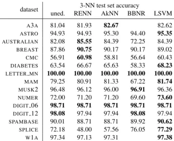
dataset 3-NN test set accuracy
uned. RENN AkNN BBNR LSVM
A3A 81.04 81.93 82.67 82.62 ASTRO 94.93 94.93 95.30 94.40 95.35 AUSTRALIAN 82.08 85.55 84.39 72.25 84.39 BREAST 87.86 90.75 90.17 90.17 89.02 CMC 56.91 60.98 58.81 56.64 60.43 DIABETES 63.54 66.67 65.63 58.33 68.23 LETTER MN 100.00 100.00 100.00 100.00 100.00 MAM 79.25 80.91 81.33 67.22 81.74 MUSK2 96.48 96.12 96.00 96.91 96.36 NUMER 72.00 71.20 71.20 69.60 73.60 DIGIT 06 98.71 98.71 98.71 98.71 98.71 DIGIT 12 98.08 97.94 97.94 98.08 97.94 SPAMBASE 90.01 88.71 88.71 89.92 90.62 SPLICE 72.18 48.00 57.56 76.05 77.29 W1A 97.34 97.13 97.31 97.38
Table 3: 3-NN generalisation accuracies for the unedited training set and for the edited training sets. The best 3-NN classification accuracy for each dataset is highlighted in bold.
Consistent with the literature starting from its introduction by Tomek (1976), AkNN appears slightly better than RENN. BBNR, on the other hand, has the poorest set of results, damaging generalisation accuracy in many cases. We believe that this is due to the fact that BBNR was designed for use in spam filtering so in the next subsection we analyse its performance in this context.
5.2 Evaluation for case-based spam filtering
We further test these noise reduction techniques in the context of spam filtering. Notice that the Local SVM classifier has been successfully applied for spam classification by Blanzieri and Bryl (2007). In addition to theSPAMBASEdataset already introduced, we use five datasets (SPAM 1-SPAM 5) from the work on spam
filtering by Delany and Bridge (2006)4.
dataset NN test set accuracy training set reduction uned. RENN AkNN BBNR LSVM RENN AkNN BBNR LSVM
SPAM 1 94.8 92.4 92.8 94.8 94.0 6.1% 4.8% 0.1% 1.7% SPAM 2 96.4 92.8 92.8 96.4 96.4 5.9% 6.7% 6.5% 3.7% SPAM 3 97.2 97.2 97.2 96.8 97.2 1.6% 3.1% 0.7% 0.9% SPAM 4 97.2 95.6 95.6 97.2 96.4 2.4% 2.5% 1.6% 1.7% SPAM 5 96.4 94.8 95.2 96.4 96.4 4.4% 4.0% 0.1% 0.7% SPAMBASE 90.0 88.7 88.7 89.9 90.6 11.2% 10.1% 7.0% 5.8%
Table 4: Generalization NN accuracies and training set reductions for spam filtering obtained with unedited training set and the training sets edited with the analysed noise reduction techniques.
The results are reported in Table 4. Apart forSPAMBASE, the editing techniques are not able to improve the generalisation accuracies of the unedited datasets. This is probably due to the fact that very little noise is present in the unedited datasets. However, it is interesting to note that BBNR degrades the accuracy only in one case, while RENN and AkNN do a fair deal of damage. The results are consistent with the experiments performed by Delany and Cunningham (2004) in which more noise is present and BBNR succeeds in improving classification performance in that case. We believe that noise reduction in spam filtering is unusual because the classes are not well separated since some spam messages have been made to look very like legitimate email. RENN and AkNN do a lot of damage in this situation as they remove
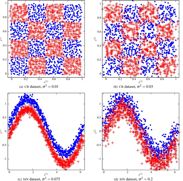
0 0.2 0.4 0.6 0.8 1 0 0.2 0.4 0.6 0.8 1 x (2 ) x(1) (a) CBdataset,σ2= 0.01 0 0.2 0.4 0.6 0.8 1 0 0.2 0.4 0.6 0.8 1 x (2 ) x(1) (b)CBdataset,σ2= 0.03 -1 -0.5 0 0.5 1 0 2 4 6 x (2 ) x(1) (c) SINdataset,σ2= 0.075 -1 -0.5 0 0.5 1 0 2 4 6 x (2 ) x(1) (d)SINdataset,σ2= 0.2
Figure 1: TheCBandSINdatasets with a subset of the different levels of Gaussian noise considered.
considerably more training data then either BBNR or LSVM and thus damage generalisation accuracy. BBNR and LSVM delete a lot less and thus have better performance. This characteristic of the LSVM strategy proves advantageous again in section 5.5 where we looks at noise reduction in the presence of unbalanced class densities.
5.3 Data with Gaussian feature noise
The objective here is to model a scenario where noise results from errors in observing and measuring the descriptive features of the samples – in the next section we cover a scenario where the errors are in the class labels assigned to the samples. In order to study the behaviour of LSVM noise reduction in the presence of ‘feature’ noise we designed two artificial datasets: the 4×4 checkerboard dataset (CB) and the sinusoid dataset (SIN). We modify the examples in the two datasets (both training and the test sets)
applying Gaussian noise with zero mean and different variance levels (σ2= 0.1, 0.2, 0.3, 0.4, 0.5 forCB
andσ2= 0.075, 0.1, 0.125, 0.15, 0.175, 0.2, 0.225, 0.25 forSIN). TheCBdata is based on an artificial data
subset of the noise configurations of the training datasets are shown in Figure 1.
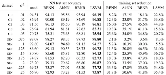
dataset σ2 NN test set accuracy training set reduction
uned. RENN AkNN BBNR LSVM RENN AkNN BBNR LSVM
CB .01 94.31 94.13 95.56 93.94 96.19 8.2% 17.1% 18.1% 22.8% CB .02 86.94 90.00 89.19 84.69 90.88 12.3% 23.0% 31.7% 33.8% CB .03 81.56 86.13 85.50 80.19 86.81 16.0% 27.5% 45.6% 44.8% CB .04 76.94 81.94 81.81 72.63 82.31 19.3% 35.1% 41.1% 15.8% CB .05 70.75 75.31 75.63 68.81 75.94 25.6% 34.0% 34.8% 20.7% SIN .075 98.07 98.27 98.33 97.73 98.80 2.1% 3.2% 3.6% 8.3% SIN .1 92.80 94.07 94.60 91.13 94.27 5.2% 10.3% 30.0% 5.5% SIN .125 86.60 89.13 90.53 78.73 90.73 11.3% 20.8% 46.5% 31.0% SIN .15 80.80 85.60 85.87 72.80 86.13 12.4% 25.5% 45.9% 36.7% SIN .175 74.87 81.53 82.20 66.33 82.73 18.3% 33.8% 47.9% 18.0% SIN .2 73.20 79.33 79.67 66.80 80.87 20.0% 33.5% 37.0% 19.3% SIN .225 69.73 73.87 77.07 63.20 77.73 33.3% 47.8% 35.8% 54.8% SIN .25 66.80 72.93 73.27 61.53 73.87 31.8% 50.6% 41.8% 35.4% Table 5: NN testing accuracies and training set reductions achieved by the analysed noise reduction tech-niques onCBandSINdatasets with samples modified by increasing Gaussian noise levels.
Table 5 reports the generalisation accuracies and the training set reductions associated with the different noise reduction techniques using a 1-NN classifier. Apart from BBNR, all the noise reduction techniques improve on the classification accuracies achievable with the unedited training set (about 5% for significant noise levels), meaning that they are all effective for Gaussian noise reduction. Moreover, our LSVM noise reduction outperforms RENN and AkNN in almost all the cases. The superiority of LSVM noise reduction in this context derives from its class discrimination capability introduced by the maximal margin principle which is tolerant to noise. In other words, a noisy sample lying in the wrong class region, is more likely to be detected by LSVM than by the other techniques based on the neighbourhood majority rule, because LSVM is able to estimate the separating hyperplane between classes and thus assess if the sample is on the right side or not.
Looking at the training set reduction rates, we can observe that, as expected, RENN and AkNN remove more samples as the variance of the noise increases. For LSVM noise reduction, instead, the reduction rates are less correlated with the Gaussian noise level; this is probably due to the different values chosen by model selection for LSVM and in particular to the C regularization parameter which is the key SVM parameter controlling the estimation of the separating hyperplane with noisy data. Moreover, with little noise, LSVM noise reduction tries to enlarge the class separation thus removing more samples.
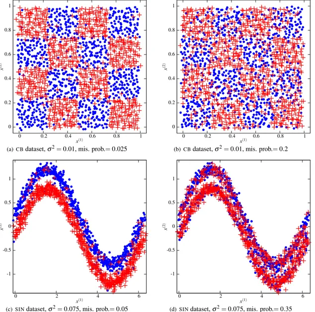
5.4 Data with mislabelled samples
In this subsection we consider noise that manifests itself as random errors in sample labelling (class noise). While the Gaussian feature noise considered in the last section affects the class boundaries, this kind of noise can show up through out the data distribution as can be seen Figure 2. We use the same artificial datasets as previously but with a minimum amount of Gaussian noise and an increasing probability of sample mislabelling. Some of the versions of the datasets used in this experiment are shown in Figure 2.
It is clear from the results shown in Table 6 that RENN, AkNN and the LSVM strategy all produce significant improvements in accuracy, improvements of more than 10% in some cases. For this reason we can conclude that the label noise is more likely to be corrected than feature noise. The differences in improvements due to RENN, AkNN and LSVM noise reduction are minimal and it is not possible to establish which is best. It is not surprising that the LSVM strategy does not dominate here as its awareness of the decision surface is useful only in the vicinity of class boundaries and many of the noisy samples in this situation are far from the boundaries. In this context the majority rule is effective and LSVM does well as it uses this principle since a local SVM model with very unbalanced data classifies all the neighbourhood with the dominant class. The fact than some mislabelled samples are located near to the class boundaries can explain the fact that LSVM noise reduction achieves the best results more frequently than the other
0 0.2 0.4 0.6 0.8 1 0 0.2 0.4 0.6 0.8 1 x (2 ) x(1)
(a)CBdataset,σ2= 0.01, mis. prob.= 0.025
0 0.2 0.4 0.6 0.8 1 0 0.2 0.4 0.6 0.8 1 x (2 ) x(1)
(b)CBdataset,σ2= 0.01, mis. prob.= 0.2
-1 -0.5 0 0.5 1 0 2 4 6 x (2 ) x(1)
(c)SINdataset,σ2= 0.075, mis. prob.= 0.05
-1 -0.5 0 0.5 1 0 2 4 6 x (2 ) x(1)
(d)SINdataset,σ2= 0.075, mis. prob.= 0.35
Figure 2: TheCBandSINdatasets with a subset of different sample mislabelling probabilities considered.
approaches (6 times against 4 times of RENN and AkNN) – however this difference is not statistically significant.
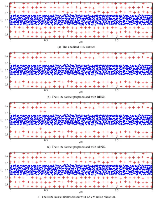
5.5 Data with unbalanced class densities
One drawback of the techniques considered here is that unbalanced class densities can have a significant impact on the effectiveness of noise reduction (Li and Hu, 2003). The problem is that there may be a tendency to remove good samples (i.e. not noise) from the minority class. Because all the techniques considered here are influenced by data density we conducted an evaluation to look at the risk of removing good samples from the minority class. We also looked at the impact of these noise reduction techniques on generalisation accuracy in the presence of unbalanced data.
We built an artificial dataset called DENwhich contains no noise but the samples in different classes
have different densities. The dataset is shown in Figure 3(a); it is created with a uniform 2-dimensional network of samples with a distance of 0.02 on each dimension for the central class and a distance of 0.06 on
dataset mislab. 1-NN test set accuracy training set reduction prob. uned. RENN AkNN BBNR LSVM RENN AkNN BBNR LSVM
CB 0.025 89.81 92.25 92.44 87.00 92.94 9.3% 21.4% 27.8% 29.7% CB 0.05 86.00 89.75 90.00 74.38 91.38 11.5% 24.3% 44.4% 35.6% CB 0.1 78.06 84.75 84.88 68.50 84.56 17.7% 35.4% 49.0% 40.0% CB 0.15 71.81 80.00 80.25 64.31 80.00 24.1% 42.0% 45.1% 51.4% CB 0.2 66.56 78.25 76.81 65.06 77.75 30.8% 46.6% 47.9% 43.3% CB 0.25 61.81 70.00 70.88 59.56 70.75 33.1% 59.6% 24.0% 24.5% SIN .075 86.60 92.87 93.00 71.46 92.93 7.5% 14.7% 58.5% 17.1% SIN .1 79.93 86.93 86.80 64.26 86.67 11.5% 21.6% 54.3% 11.4% SIN .125 74.40 83.13 83.93 59.66 84.00 17.7% 32.5% 51.9% 29.9% SIN .15 68.13 78.00 77.00 56.07 77.73 18.8% 38.7% 58.4% 24.7% SIN .175 62.13 75.00 74.80 54.87 75.60 25.7% 51.3% 42.8% 35.9% SIN .2 56.53 70.27 69.47 55.80 69.80 31.9% 62.1% 32.3% 46.3% SIN .225 54.47 63.13 63.07 54.73 63.33 37.5% 70.3% 30.3% 37.0% SIN .25 54.80 58.53 60.73 56.20 61.33 47.0% 80.1% 22.1% 58.0%
Table 6: NN testing accuracies and training set reduction achieved by the analysed noise reduction tech-niques on the CB and SIN datasets with samples modified by increasing levels of sample mislabelling probability.
each dimension for the peripheral class, and applying Gaussian noise withσ2= 0.005 to all the samples.
Figure 3(b) shows the behaviour of the RENN algorithm which removes almost all the samples of the external class that are closest to the internal class. Although the separation between classes is enlarged, this is achieved by removing only samples of the less dense class and it is clear that the generalisation capability of the edited set is extremely deteriorated. This behaviour is not caused by model selection problems as it will happen across a range of k values because the majority class will always out vote the minority class. The AkNN results shown in Figure 3(c) are very similar to those for RENN. This is not surprising because the same considerations discussed for RENN hold for AkNN as well.
The application of LSVM noise reduction on theDENdataset is shown in Figure 3(c). We can observe that only 3 samples are incorrectly removed, meaning that the local SVM is able to correctly separate the classes in the neighbourhood of a borderline sample even in the presence of uneven class densities. While the LSVM strategy is performing well here it has been proposed for example by Osuna et al (1997) to modify the penalty parameter of SVM for unbalanced data to further increase the generalisation accuracy. In fact, by increasing the penalty score associated with the peripheral class, the LSVM performance can be improved so that it does not delete any instances of the minority class.
dataset NN test set accuracy training set reduction uned. RENN AkNN LSVM RENN AkNN LSVM
MUSK2 96.24 96.24 95.76 96.42 4.6% 4.6% 2.6% MUSK2 unbal. 96.12 94.24 94.91 95.33 1.9% 1.9% 1.4%
ASTRO 93.93 94.75 95.03 94.98 4.5% 4.5% 2.5%
ASTROunbal. 88.23 86.98 87.75 89.20 2.9% 2.9% 2.8%
Table 7: Generalization accuracies of the NN classifier using the unedited training sets and the analysed noise reduction techniques on theMUSK2 andASTROdatasets in the original version and in the unbalanced class densities version.
In order to understand the behaviour of the noise reduction techniques on real data with different class densities, we selected from the datasets of section 5.1 two datasets with a considerable number of sam-ples and on which RENN and AkNN performs similarly to the LSVM-based strategy. The datasets are
MUSK2 andASTRO, and we modified them by randomly removing 75% of samples of the already less
pop-ulated class thus obtaining two datasets with unbalanced class densities. The results of the noise reduction techniques (for LSVM noise reduction the class penalties are not modified) are shown in Table 7. While the three techniques achieve very similar test classification results with the original datasets LSVM noise
0.3 0.4 0.5 0.6 0.7 0 0.5 1.5 2 x (2 ) x(1)
(a) The uneditedDENdataset.
0.3 0.4 0.5 0.6 0.7 0 0.5 1.5 2 x (2 ) x(1)
(b) TheDENdataset preprocessed with RENN.
0.3 0.4 0.5 0.6 0.7 0 0.5 1.5 2 x (2 ) x(1)
(c) TheDENdataset preprocessed with AkNN.
0.3 0.4 0.5 0.6 0.7 0 0.5 1.5 2 x (2 ) x(1)
(d) TheDENdataset preprocessed with LSVM noise reduction.
Figure 3: The uneditedDENdataset and the noise reduction preprocessed versions.
reduction is clearly better than RENN and AkNN for the unbalanced versions. The results confirm the robustness of LSVM noise reduction for unbalanced class densities.
6 Conclusions
We presented a novel noise reduction technique, called LSVM noise reduction, based on the probabilistic output of the Local Support Vector Machine classifier trained on the neighbourhood of each training set
sample. The evaluation shows that this approach is able to improve with statistical significance the gener-alisation accuracy of 1-NN and 3-NN classifiers on a number of real datasets and on artificial datasets with increasing levels of noise in both features and labels. We selected AkNN, RENN and BBNR as the alter-native noise reduction techniques against which we would evaluate our new strategy. We selected AkNN and RENN because, while there are other strategies that achieve better reduction in training set size, these are most effective at improving generalisation accuracy (Wilson and Martinez, 1997). We chose BBNR be-cause we are interested in spam filtering, the application area where that technique originates and bebe-cause we were curious about why its good performance there is not reproduced in other application areas. LSVM noise reduction has shown to be more effective that AkNN and RENN for general datasets, for Gaussian noise, for data with different class densities and, together with BBNR, in the specific field of spam filtering. Since this LSVM strategy can be applied for redundancy reduction as well, we aim to develop and evaluate it for the competence preservation where the main objective is storage minimization. Moreover, for large and noisy datasets, LSVM can be used in a two-stage SVM strategy in which the LSVM noise reduction is used before the global SVM training as already proposed by Bakir, Bottou, and Weston (2005) and by Sriperumbudur and Lanckriet (2007) who use traditional noise reduction methods. The purpose of LSVM noise reduction, in this case, is to remove the points that are very likely to be considered support vectors in training a global SVM in order to enlarge the class separation. In this way the linear dependency between the number of support vectors and the training set cardinality is broken, and so the global SVM kernel matrix has a better chance of fitting into memory and thus dramatically speeding up the SVM training and testing phase.
References
Aha DW, Kibler D, Albert MK (1991) Instance-based learning algorithms. Mach Learn 6(1):37–66 Angiulli F (2007) Fast nearest neighbor condensation for large data sets classification. IEEE Transactions
on Knowledge and Data Engineering 19(11):1450–1464 Asuncion A, Newman DJ (2007) Uci machine learning repository
Bakir GH, Bottou L, Weston J (2005) Breaking SVM complexity with cross-training. In: Saul LK, Weiss Y, Bottou L (eds) Advances in Neural Information Processing Systems 17, MIT Press, Cambridge, MA, pp 81–88
Bello-Tom´as JJ, Gonz´alez-Calero PA, D´ıaz-Agudo B (2004) JColibri: An Object-Oriented Framework for Building CBR Systems. In: ECCBR, pp 32–46
Blanzieri E, Bryl A (2007) Evaluation of the highest probability SVM nearest neighbor classifier with variable relative error cost. In: CEAS 2007, Mountain View, California
Blanzieri E, Melgani F (2006) An adaptive svm nearest neighbor classifier for remotely sensed imagery. In: Geoscience and Remote Sensing Symposium, 2006. IGARSS 2006. IEEE International Conference on, pp 3931–3934
Blanzieri E, Melgani F (2008) Nearest neighbor classification of remote sensing images with the maximal margin principle. Geoscience and Remote Sensing, IEEE Transactions on 46(6):1804–1811
Bottou L, Vapnik V (1992) Local learning algorithms. Neural Comput 4(6):888–900
Brighton H, Mellish C (2002) Advances in instance selection for instance-based learning algorithms. Data Mining and Knowledge Discovery 6(2):153–172
Brodley CE (1993) Addressing the selective superiority problem: Automatic algorithm/model class selec-tion. In: Tenth International Machine Learning Conference, Amherst, MA, pp 17–24
Cabailero Y, Bello R, Garcia MM, Pizano Y, Joseph S, Lezcano Y (2005) Using rough sets to edit training set in k-nn method. In: Intelligent Systems Design and Applications, 2005. ISDA ’05. Proceedings. 5th International Conference on, pp 456–461
Cameron-Jones RM (1995) Instance selection by encoding length heuristic with random mutation hill climbing. In: Eighth Australian Joint Conference on Artificial Intelligence, pp 99–106
Cao G, Shiu S, Wang X (2001) A fuzzy-rough approach for case base maintenance
Cataltepe Z, Abu-mostafa YS, Magdon-ismail M (1999) No free lunch for early stopping. Neural Compu-tation 11:995–1009
Chang CC, Lin CJ (2001) LIBSVM: a library for support vector machines
Chang CL (1974) Finding prototypes for nearest neighbor classifiers. Computers, IEEE Transactions on C-23(11):1179–1184
Chou CH, Kuo BH, Chang F (2006) The generalized condensed nearest neighbor rule as a data reduction method. In: ICPR ’06: Proceedings of the 18th International Conference on Pattern Recognition, IEEE Computer Society, Washington, DC, USA, pp 556–559
Cortes C, Vapnik V (1995) Support-vector networks. Mach Learn pp 273–297
Cunningham P, Doyle D, Loughrey J (2003) An evaluation of the usefulness of case-based explanation. In: In Proceedings of the Fifth International Conference on Case-Based Reasoning, Springer, pp 122–130 Delany SJ, Bridge D (2006) Textual case-based reasoning for spam filtering: A comparison of
feature-based and feature-free approaches. Artificial Intelligence Review 26(1-2):75–87
Delany SJ, Cunningham P (2004) An analysis of case-based editing in a spam filtering system. In: Funk P, Gonz´alez-Calero P (eds) Advances in Case-Based Reasoning, 7th European Conference on Case-based Reasoning (ECCBR 2004), Springer, LNAI, vol 3155, pp 128–141
Demsar J (2006) Statistical comparisons of classifiers over multiple data sets. J Mach Learn Res 7:1–30 D´ıaz-Agudo B, Gonz´alez-Calero P, Recio-Garc´ıa J, S´anchez A (2007) Building cbr systems with jcolibri.
Special Issue on Experimental Software and Toolkits of the Journal Science of Computer Programming 69(1-3):68–75
Gamberger A, Lavrac N, Dzeroski S (2000) Noise detection and elimination in data preprocessing: exper-iments in medical domains. Applied Artificial Intelligence pp 205–223
Gates G (1972) The reduced nearest neighbor rule. Information Theory, IEEE Transactions on 18(3):431– 433
Genton MG (2001) Classes of kernels for machine learning: A statistics perspective. J Mach Learn Res 2:299–312
Hao X, Zhang C, Xu H, Tao X, Wang S, Hu Y (2008) An improved condensing algorithm. In: Computer and Information Science, 2008. ICIS 08. Seventh IEEE/ACIS International Conference on, pp 316–321 Hart P (1968) The condensed nearest neighbor rule. Information Theory, IEEE Transactions on 14(3):515–
516
Huang D, Chow TWS (2005) Enhancing density-based data reduction using entropy. Neural Comp 18(2):470–495
Jiang Y, Zhou Z (2004) Editing training data for knn classifiers with neural network ensemble. In: Advances in Neural Networks ISNN 2004, Springer, LNCS, vol 3173, pp 356–361
Koplowitz J, Brown TA (1981) On the relation of performance to editing in nearest neighbor rules. Pattern Recognition 13(3):251–255
Leake DB (1996) CBR in context: The present and future. In: Leake DB (ed) Case Based Reasoning: Experiences, Lessons, and Future Directions, MIT Press, pp 3–30
Lee Y, Mangasarian O (2001) SSVM: A Smooth Support Vector Machine for Classification. Computational Optimization and Applications 20(1):5–22
Li RL, Hu JF (2003) Noise reduction to text categorization based on density for knn. In: Machine Learning and Cybernetics, 2003 International Conference on, vol 5, pp 3119–3124 Vol.5
Lin HT, Lin CJ, Weng R (2007) A note on platt’s probabilistic outputs for support vector machines. Mach Learn 68(3):267–276
Lorena AC, Carvalho ACPLFd (2004) Evaluation of noise reduction techniques in the splice junction recog-nition problem. Genetics and Molecular Biology 27:665 – 672
Lowe DG (1995) Similarity metric learning for a variable-kernel classifier. Neural Comput 7(1):72–85 Malossini A, Blanzieri E, Ng RT (2006) Detecting potential labeling errors in microarrays by data
pertur-bation. Bioinformatics 22(17):2114–2121
McKenna E, Smyth B (2000) Competence-guided case-base editing techniques. In: EWCBR ’00: Proceed-ings of the 5th European Workshop on Advances in Case-Based Reasoning, Springer-Verlag, London, UK, pp 186–197
Mitra P, Murthy CA, Pal SK (2002) Density-based multiscale data condensation. Pattern Analysis and Machine Intelligence, IEEE Transactions on 24(6):734–747
Nugent C, Doyle D, Cunningham P (2008) Gaining insight through case-based explanation. Journal of Intelligent Information Systems
Osuna EE, Freund R, Girosi F (1997) Support vector machines: Training and applications
Pan R, Yang Q, Pan SJ (2007) Mining competent case bases for case-based reasoning. Artificial Intelligence 171(16-17):1039–1068
Park J, Im K, Shin C, Park S (2004) MBNR: Case-Based Reasoning with Local Feature Weighting by Neural Network. Applied Intelligence 21(3):265–276
Pawlak Z (1991) Rough Sets: Theoretical Aspects of Reasoning about Data, 1st edn. Springer
Pechenizkiy M, Tsymbal A, Puuronen S, Pechenizkiy O (2006) Class noise and supervised learning in med-ical domains: The effect of feature extraction. In: CBMS ’06: Proceedings of the 19th IEEE Symposium on Computer-Based Medical Systems, IEEE Computer Society, Washington, DC, USA, pp 708–713 Platt JC (1999a) Fast training of support vector machines using sequential minimal optimization. MIT Press
Cambridge, MA, USA pp 185–208
Platt JC (1999b) Probabilistic outputs for support vector machines and comparisons to regularized likeli-hood methods. In: Advances in Large Margin Classifiers, pp 61–74
Quinlan J (1986) The effect of noise on concept learning. In: Michalski R, Carboneel J, Mitchell T (eds) Machine Learning, Morgan Kaufmann
Ritter G, Woodruff H, Lowry S, Isenhour T (1975) An algorithm for a selective nearest neighbor decision rule. Information Theory, IEEE Transactions on 21(6):665–669
Roth-Berghofer T (2004) Explanations and case-based reasoning: Foundational issues. In: Funk P, Gonz´alez-Calero PA (eds) Advances in Case-Based Reasoning, Proceedings of the 7th European Confer-ence on Case-based Reasoning, ECCBR 2004, Springer, Lecture Notes in Computer SciConfer-ence, vol 3155, pp 389–403
Salam´o M, Golobardes E (2001) Rough sets reduction techniques for case-based reasoning. In: Aha DW, Watson I (eds) Case-Based Reasoning Research and Development, Proceedings 4th International Con-ference on Case-Based Reasoning, ICCBR 2001, Springer, Lecture Notes in Computer Science, vol 2080, pp 467–482
Salam´o M, Golobardes E (2002) Deleting and building sort out techniques for case base maintenance. In: Craw S, Preece AD (eds) Advances in Case-Based Reasoning, Proceedings of 6th European Conference, ECCBR 2002 Aberdeen, Scotland, UK, September 4-7, 2002,, Springer, Lecture Notes in Computer Science, vol 2416, pp 365–379
Salam´o M, Golobardes E (2004) Global, local and mixed rough sets case base maintenance techniques. In: Proceedings of the 6th Catalan Conference on Artificial Intelligence, IOS Press, pp 127–134
S´anchez JS, Barandela R, Marqu´es AI, Alejo R, Badenas J (2003) Analysis of new techniques to obtain quality training sets. Pattern Recognition Letters 24(7):1015–1022
Schlkopf B, Smola AJ (2001) Learning with Kernels: Support Vector Machines, Regularization, Optimiza-tion, and Beyond (Adaptive Computation and Machine Learning). The MIT Press
Segata N, Blanzieri E (2007) Operators for transforming kernels into quasi-local kernels that improve SVM accuracy. Tech. rep., DISI, University of Trento
Segata N, Blanzieri E (2008) Empirical assessment of classification accuracy of Local SVM. Tech. Rep. DISI-08-014, Dipartimento di Ingegneria e Scienza dell’Informazione, University of Trento, Italy Smyth B, Keane M (1995) Remembering to forget: A competence preserving case deletion policy for cbr
system. In: Mellish C (ed) Proceedings of the Fourteenth International Joint Conference on Artificial Intelligence, IJCAI (1995), Morgan Kaufmann, pp 337–382
Sriperumbudur BK, Lanckriet G (2007) Nearest neighbor prototyping for sparse and scalable support vector machines. Tech. rep., Dept. of ECE, UCSD
Tang S, Chen SP (2008a) Data cleansing based on mathematic morphology. In: Bioinformatics and Biomedical Engineering, 2008. ICBBE 2008. The 2nd International Conference on, pp 755–758 Tang S, Chen SP (2008b) An effective data preprocessing mechanism of ultrasound image recognition. In:
Bioinformatics and Biomedical Engineering, 2008. ICBBE 2008. The 2nd International Conference on, pp 2708–2711
Tomek I (1976) An experiment with the edited nearest-neighbor rule. Systems, Man and Cybernetics, IEEE Transactions on 6(6):448–452
Vapnik V (1991) Principles of risk minimization for learning theory. In: NIPS, pp 831–838
Vapnik V (1999) The Nature of Statistical Learning Theory (Information Science and Statistics). Springer Wilcoxon F (1945) Individual comparisons by ranking methods. Biometrics 1(6):80–83
Wilson DL (1972) Asymptotic properties of nearest neighbor rules using edited data. Systems, Man and Cybernetics, IEEE Transactions on 2(3):408–421
Wilson DR, Martinez TR (1997) Instance pruning techniques. In: Machine Learning: Proceedings of the Fourteenth International Conference (ICML-97), pp 403–411
Wilson DR, Martinez TR (2000) Reduction techniques for instance-based learning algorithms. Mach Learn 38(3):257–286
Zhang J (1992) Selecting typical instances in instance-based learning. In: ML92: Proceedings of the ninth international workshop on Machine learning, Morgan Kaufmann Publishers Inc., San Francisco, CA, USA, pp 470–479