P
HD T
HESISDevelopment, validation and application of
accurate molecular force fields for complex soft
matter systems
Author:
Gianluca DELFRATE
Supervisor:
Prof. Vincenzo BARONE
Dr. Giordano MANCINI
A thesis submitted in fulfillment of the requirements for the degree of Doctor of Philosophy in
Contents
Preface 1
Introduction 2
I THEORY 5
1 Molecular Mechanics force fields 9
1.1 Force field terms . . . 10
1.1.1 Bonded interactions . . . 10
1.1.2 Non-bonded interactions . . . 11
van der Waals interactions . . . 11
Electrostatic interactions . . . 14
1.2 A survey of existing force fields . . . 15
1.2.1 Biomolecules . . . 16
1.2.2 Water models . . . 17
1.2.3 Minerals . . . 17
1.2.4 Reactive force fields . . . 17
1.2.5 Polarizable models . . . 17
1.2.6 Algorithms for high-quality FFs . . . 18
2 Molecular Dynamics 19 2.1 Integration of the equations of motion . . . 19
2.2 Boundary Conditions . . . 21
2.3 Long range electrostatics . . . 22
2.4 Geometric constraints . . . 23
2.5 Starting conditions . . . 23
2.6 Temperature and Pressure control . . . 24
3 Force field development 27 3.1 Joyce . . . 27
3.1.1 An overview . . . 27
3.1.2 Current compatibilities . . . 28
3.1.3 Parametrization protocol and validation . . . 29
3.2 LRR-DE . . . 31
3.2.1 The Linear Ridge Regression Differential Evolution procedure . . . 32
Optimization of the hyperparameters using differential evolution . . . 34
Properties of LRR-DE . . . 36
3.2.2 Single-objective application of the LRR-DE procedure: the force-matching approach 37 3.2.3 Generalization to the multi-objective fitting . . . 38
Optimization of the weights in the multi-objective fitting . . . 40
4 Analysis of trajectories 41 4.1 Structural properties . . . 41
4.2 Dynamical properties . . . 42
4.3 Hydrogen bond analysis . . . 43
4.4 Absorption spectra . . . 44
4.5 Free energy calculations . . . 44
4.6 Clustering analysis of structures . . . 46
II Applications 49 5 Dissociation of Doxorubicin from DNA Binding Site 53 5.1 Background . . . 53
5.1.1 Visualization in chemistry . . . 53
5.1.2 The Caffeine molecular viewer: an overview . . . 54
5.2 The DOX/DNA system . . . 55
5.2.1 Doxorubicin . . . 55
5.2.2 Computational Details . . . 55
5.2.3 Results . . . 57
The unbinding mechanism . . . 57
Studying the dissociation process in a IVR environment . . . 59
5.2.4 Conclusions . . . 60
6 Fine-Tuning of Atomic Point Charges: the Case of Pyridine 63 6.1 Background . . . 63 6.2 Methods . . . 64 6.3 Results . . . 66 6.3.1 Aqueous solution . . . 66 6.3.2 Pure pyridine . . . 67 6.3.3 Conclusion . . . 70
7 Modeling of Photoactive Dyes Within a Sunlight Harvesting Device 73 7.1 Background . . . 73
7.2 Methods . . . 75
7.2.1 General approach . . . 75
7.2.2 QM calculations . . . 76
7.2.3 Molecular modeling and MD simulations . . . 77
7.3.1 Fluorophore force fields . . . 78
7.3.2 MD simulation analysis . . . 79
7.3.3 UV absorption spectra . . . 83
7.3.4 Conclusion . . . 85
8 Computational Study of a Fluorescent Molecular Rotor in Various Environments 87 8.1 Background . . . 87
8.2 Methods . . . 89
8.2.1 QM calculations and force field parameterization . . . 89
8.2.2 MD simulations . . . 89
8.3 Results and Discussion . . . 91
8.3.1 DPAP force field . . . 91
8.3.2 DPAP in solutions . . . 93
8.3.3 DPAP in polymeric matrix and lipid bilayer . . . 96
8.3.4 Comparison of the structural and dynamic features of DPAP in multiple environ-ments . . . 98
8.3.5 Optical absorption spectra of DPAP . . . 101
8.4 Conclusions . . . 105
9 Validation of the LRR-DE procedure 107 9.1 Background . . . 107
9.1.1 Current status of parameterization procedures of non-bonded metal ions force fields . . . 108
9.2 GRASP sampling . . . 109
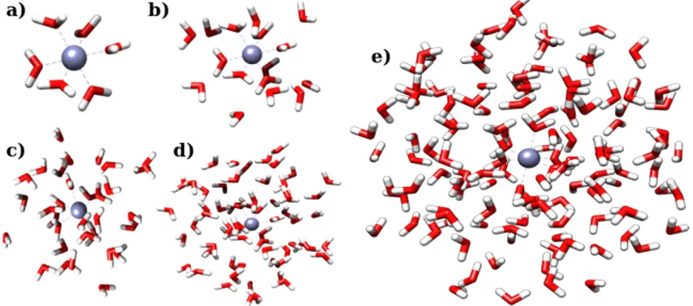
9.2.1 Generation of the candidate configurations . . . 109
9.2.2 The metal-centric dissimilarity score . . . 110
The dimensionality reduction and permutational symmetry . . . 111
9.2.3 The combinatorial optimization of the training set . . . 111
9.3 Computational details . . . 111
9.4 Validation . . . 112
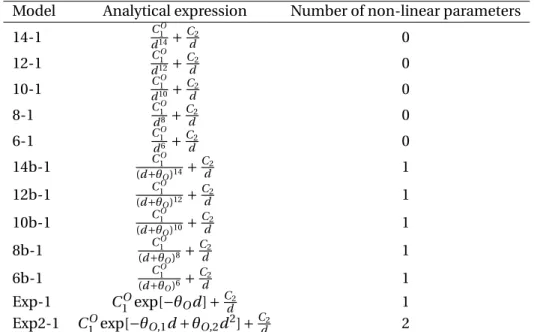
9.4.1 Systematic comparative study of binary potentials . . . 114
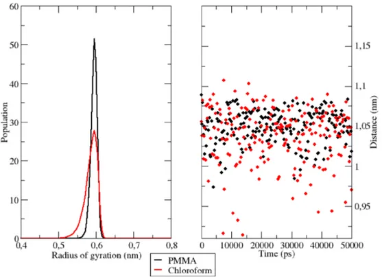
9.4.2 Parameters Optimization and Molecular Dynamics simulations . . . 119
9.5 Conclusion . . . 124
Conclusions and perspectives 125 III Appendices 127 A Force field parameters 129 A.1 AP dyes . . . 129
A.2 DPAP . . . 133
Preface
Up to now, the methodologies and results here discussed have led to the following publications: • F. Fracchia, G. Del Frate4, G. Mancini, W. Rocchia, V. Barone, "Force Field Parametrization of
Metal Ions From Statistical Learning Technique", Journal of Chemical Theory and Computation, 2017, Just accepted, DOI: 10.1021/acs.jctc.7b00779 (4co-first author)
• M. Macchiagodena, G. Del Frate*, G. Brancato, B. Chandramouli, G.Mancini, V. Barone, "Com-putational Study of DPAP Molecular Rotor in Various Environments: From Force Field Develop-ment to Molecular Dynamics Simulations and Spectroscopic Calculations", Physical Chemistry
Chemical Physics, 2017, Just accepted, DOI: 10.1039/C7CP04688J (*corresponding author)
• M. Macchiagodena, G. Mancini, M. Pagliai, G. Del Frate, V. Barone, "Fine-tuning of atomic point charges: Classical simulations of pyridine in different environments", Chemical Physics Letters, 2017, 677, 120
• A. Salvadori, G. Del Frate, M. Pagliai, G. Mancini, V. Barone, "Immersive virtual reality in compu-tational chemistry: Applications to the analysis of QM and MM data", International Journal of
Quantum Chemistry, 2016, 116, 1731
• G. Del Frate, F. Bellina, G. Mancini, G. Marianetti, P. Minei, A. Pucci, V. Barone, "Tuning of dye op-tical properties by environmental effects: a QM/MM and experimental study", Physical
Introduction
In the last decades, computational chemistry has established itself as an useful and powerful tool for designing molecular systems and forecast their properties over a wide range of space and time scales. In silico methods accelerate the design and discovery of novel materials with specific proper-ties (e.g., mechanical, optical, pH responsive) as well as new chemicals with pharmacological activity. The proper theoretical framework for the description of molecular systems at the atomic level are the laws of quantum mechanics (QM). However, a satisfactory sampling of the phase space of large sys-tems (up to a milion of atoms) is achievable only by employing classical methods, such as Molecular Dynamics (MD) and Monte Carlo (MC) simulations [1]. These techniques are based on molecular me-chanics (MM) rules, which assume molecules being composed by a set of atoms modeled as spheres and linked together by springs. Electronic degrees of freedom are neglected, as entailed by the Born-Oppenheimer approximation. Atomic motions are described by means of the classical laws, and the potential energy surface (PES) is represented by a sum of analytical expressions with immediate phys-ical meaning, aimed at describing bonded and non-bonded interactions between atoms. The integra-tion the classical equaintegra-tion of mointegra-tion is rather cheap, thus to allow to get structural and thermodynamic properties in molecular simulations at a computational cost which is significantly lower if compared to QM and hybrid QM/MM computations.
The complete set of functions and the corresponding parameters used in MM methods to describe both intra- and intermolecular interactions in a chemical system is named force field (FF). At present, a high number of FFs is available in computational chemistry, each to be used in a wide, yet specific chemical domain, from organic liquids (as the OPLS force field [2, 3]) to biomolecules (e.g., AMBER [4, 5] and GROMOS [6]) and minerals (e. g. INTERFACE [7], ClayFF [8]). In each of them, atoms are organized in "atom types", i.e. chemical elements with a specific hybridization and a specific chemical surrounding: identical atom types share the same FF parameters, and the same atoms (e.g., carbon) can be described by multiple atom types (e.g., in a sp2carbonyl group or in a sp alkyne). Transferability of both functional forms and parameters is an important feature, since it enables the employment of parameters developed on a small set of molecules to a wider range of chemical entities. The accuracy offered by transferable force fields however is limited by many factors (first of all, the similarity of the target molecule to those employed in the parameterization route and the thermodynamic conditions employed in the simulations during the parameterization procedure) and it may be also insufficient to guarantee the reproduction of several target properties of interest at the same level of the species included in the training set. Moreover, the invoked generality of the parameters may undermine the simulation of several chemical phenomena, such as spectroscopic data, the change of flexibility of organic dyes when going from liquid solutions to more obstructing environments, and bulk properties of liquids (as the static dielectric constant², density, structure, and many others).
has become ever more relevant in life and material science. Increasingly complex systems can be simu-lated by exploiting highly performing computing (HPC) facilities. In this scenario, there is wide margin for improve the currently available MM models and gather new insights from theoretical investigations with more detail and accuracy. Therefore, it is no coincidence that novel fitting methods and strate-gies, aimed at overcoming the drawbacks mentioned above, have been developed in the last few years: among them, innovative tools and software for the development of intramolecular FFs specifically tai-lored for one molecule by fitting QM optimized energies, gradients and Hessian matrix have recently attracted attention within the scientific community [9–13]. Parallel efforts are directed to the refine-ment or the computation ex novo of atomic charges [14], through the employrefine-ment of novel schemes for electron density partitioning [15] or to the inclusion of virtual sites, which mimic somehow polar-izability effects and correctly simulate hydrogen bonding patterns, within molecular topologies [16].
This thesis is devoted to improve classical simulations reliability through the application of novel strategies for classical FFs optimization. To this end, MM and QM state of the art approaches have been combined together and integrated in different protocols, devoted to the accurate parameteriza-tion and classical MD simulaparameteriza-tions of molecular systems, to overcome current performances offered by general parameters and to address new chemical problems of different kind. With this aim, the employed FFs have been developed from scratch or re-parameterized only in some parts depending on the circumstances, and showing how an accurate modeling, based on first principle computations and not relying on any empirical parameters, allow to compute with accuracy a series of thermody-namic, structural and spectroscopic properties of interest. In order to validate the optimized set of parameters, the computed MD trajectories have been extensively investigated: the reliability of the proposed parameters has been evaluated by comparing simulated results with available experimen-tal data. In the cases of molecular probes force field optimization, the population of QM-predicted conformational energy minima along the trajectory has also been considered. Furthermore, MD has been opportunely integrated with QM methods (mainly routed in the density functional theory, DFT) to compute absorption spectra, which are not obtainable with standard force field-based procedures, in order to gain a further comparison with experiments.
The thesis is organized as follows. In the first part, the theory underlying the thesis work is briefly reported. The second part focuses on the applications arising from the protocols explained in the first part. The chemical investigations carried out in the course of this PhD are reported following, in as-cending order, a sort of "degree of modification" of the used parameter set, from the first works (where a low level of modification of the FF is applied) until to the last one, where a totally new parameteriza-tion procedure is proposed.
Future perspectives concerning this research work are given in the last section. All the parameter sets developed in this thesis are given in the Appendice.
Part I
THEORY
This part is organized as follows. In Chapter 1, a summary on classical force fields and most com-mon functional forms currently available in the literature is given. In Chapter 2 a general overview on MD technique (the main tool used in this thesis) is briefly reported. In this regard, MD simulations have been used to
1. validate the developed FFs;
2. investigate on structural, dynamic and spectroscopic properties of the considered chemical sys-tems.
Chapter 3 presents two algorithms for force field development: Joyce [9], which performs a parameter optimization for the FF intramolecular potential, and LRR-DE, a new procedure for the generation of non-bonded models for metal ions, developed in the course of this PhD. The analysis of the MD trajectories have been performed by using a set of computational tools, which are outlined in Chapter 4.
Chapter 1
Molecular Mechanics force fields
The total energy E of a molecular system is given by the time-independent Schrödinger equation ˆ
HΨ(r,R) = EΨ(r,R) (1.1)
where ˆH is the Hamiltonian operator which describes both potential and kinetic energy and Ψ is
the wavefunction dependent on the electrons and the nuclei positions (r and R). Under the Born-Oppenheimer assumption, the motion of electrons can be separated from the motion of the nuclei, due to the large difference between elctron and nuclear masses: electrons moves faster and they readapt their positions instantly to nuclear motions. Therefore, the wave function can be factorized into an electronic and a nuclear part, and the electronic energy (Eel) can be computed for fixed nuclear po-sitions. Eel defines the PES over all the possible nuclear coordinates: a chemical systems can be con-sidered as a ball moving on the corresponding PES, whose sampling by means of dynamic simulations allow to get a lot of molecular properties.
At present, several approximation levels can be used in order to model the PES (from MM to DFT and coupled-cluster methods). In force field methods, it is calculated as a sum of pairwise potentials, dependent on the spatial coordinates of the nuclei. The specific decomposition depends upon the force field in use. One way of representing the potential energy of a molecule in vacuum is the follow-ing:
Ei nt r a= Est r et ch+ Ebend+ ER t or s+ EF t or s+ Enb (1.2) Here, the intramolecular energy depends on five terms: the first four are due to bonded-atoms in-teractions, and single energy contributions derive from displacement from equilibrium values. Est r et ch,
Ebend, ER t or s and EF t or s correpond to the stretching, bending, rigid and flexible torsions potentials. The last (Enb) term refers to non-bonded contributions: both 1-4 interactions (computed between end atoms involved in a dihedral angles, often scaled applying an empirical factor) and those between atoms separated by more than three bonds are included in such term. The first derivative of the po-tential Ei nt r acomputed on atom i corresponds to the atomic force on that atom.
Eq. 1.2 refers to a particular class of force field, i.e. the empirical non-reactive ones. Such kind of classical models have been used within this work: the corresponding terms, well adopted within widespread MD codes, are discussed in the next section. It has to be stressed that alternative ways of modeling the PES of a system, such as polarizable and reactive models, can be adopted depending on the chemical phenomenon that needs to be studied.
1.1 Force field terms
1.1.1 Bonded interactions
The most known approach to model chemical bonds in a molecule is to rely on Hooke’s law formula, which assign quadratic penalties to the displacement from the reference bond length, according to
V (r ) =1 2k s i j(bi j− b eq i j) 2 (1.3)
where ki js is the force constant associated to the i j bond, bi jis the measured bond length and beqi j is the bond length at the equilibrium. Anharmonic potentials too, with asymmetric energy profile and zero forces at infinite distance can also be used. Among them, the Morse potential [17], has the following form
V (r ) = Di j[1 − exp(−βi j(bi j− beqi j))]2 (1.4) where Di jandβi jare the well depth and the corresponding steepness, respectively. The Morse poten-tial is used to describe bond formation and bond breaking, since it considers the existence of unbound states: for this reason it is adopted in reactive force fields in modeling chemical reactivity.
The Hooke’s law is used also to describe deviation of angles from their equilibrium values:
V (θ) =1 2k θ i j k(θi j k− θ eq i j k) 2 (1.5)
where ki j kθ is the force constant of angle cijk, θi j k andθeqi j k are actual angle and corresponding refer-ence value. Boradly speaking, values of kθi j k are generally lower if compared to ki j ks , meaning that lower amounts of energy are required to deform angles and move them from their reference positions. GROMOS force field uses a cosine-based function for angle vibrations. A harmonic corrective term on the distance between i and k (i.e., the end atoms of the angle), in addition to Eq. 1.5, is used in the CHARMM force field [18] (known as the Urey-Bradley potential).
In flexible molecules, dihedral angles affect molecular conformation. Two different kind of dihedral angles can be defined: rigid torsions, modeled through standard harmonic potentials, as the ones described by equation 1.3 and 1.5, and flexible torsions. Improper dihedral angles, often included in force fields in order to keep a group of atoms fixed at a particular geometry (e.g., planar aromatic rings), are included in the first category. In the other one, dihedral angles are modeled using periodic functions (cosine series expansion). A typical form is the following:
EFt or s= ki j klφ (1 + cos(nφ − γ)) (1.6)
Here, ki j klφ is the force constant which governs the flexible torsion defined by the i , j , k and l atoms.γ is the phase factor, and it determines where the function passes thorugh a minimum. The multiplicity value instead defines the number of minima along a complete scan of the i j kl dihedral angle. Mag-nitudes of kφi j klare notably lower if compared to bonds and angles force constants: for some systems, significant deviations of dihedral angles from their equilibrium states can be easily observed in MD simulations of few hundreds of picoseconds.
The parameterization of the bonded interactions is usually performed by means of spectroscopic experiments: also quantum mechanics calculations on the isolated molecule can be used.
1.1.2 Non-bonded interactions
Non-bonded interactions are essentially of van der Waals (vdW) and electrostatic nature. Usually mod-elled as a function of the inverse of the distance beetween two bonded atoms, force field non-bonded part is important for chemical structure determination: in fact, both van der Waals and elec-trostatic interactions have a key role in determining the global structure of large molecules, e.g. pro-tein folding. Furthermore, they contribute to intermolecular interactions and macroscopic properties. vdW interactions, in particular, have been shown to dominate the heats of vaporization of nonpolar organic molecules and have effects on several other condesed-phase properties, such as density and molecular volumes.
Depending on the force field in use, 1-4 interactions (i.e., those between non-bonded atoms which are separated by three bonds) can be scaled down by using empirical factors. Just for example, OPLS uses a 0.5 scale factor for both electrostatic and vdW interactions; AMBER applies 0.8333 for electro-statics, while it scales vdW in equal measure as OPLS. Scale factors for non-bonded interactions are not considered in GROMOS force field.
van der Waals interactions
The most common way to think about vdW forces is to consider two non-bonded atoms. In a clas-sical way, such atoms could be seen as two spheres with an atomic radius, rvdW: at infinte distances there are no attractive forces between them. As the two atoms approach one another, dispersive forces beetween them arise, mainly due to the correlated fluctuations of the electron clouds. This results in the formation of two dipoles. Such interactions are commonly named London forces and they have an inverse sixth power dependence on the distance between the two considered atoms [19]. The most popular function used to describe Van der Waals interactions is the Lennard-Jones potential [20] (Eq. 1.7). V (r ) = 4²i j ·µσ i j ri j ¶12 − µσ i j ri j ¶6¸ (1.7) In such equation, rijindicates the distance beetween the considered atoms i and j,σi jis the separation at which the energy value is zero and²i j is the minimum (the well depth). The well depth parameter is often expressed in units of temperature, as²/kb, where kb is the Boltzmann’s constant. Often, the same law is expressed in function of the distance at which the energy value matches the well depth, rm. In this case, the LJ function is
V (r ) = ²i j ·µr m ri j ¶12 − 2 µr m ri j ¶6¸ (1.8) It is easy to demonstrate that the value of rm correspond to 21/6σ, since, at this separation, the first derivative of the energy with respect to the distance r is equal to zero.
The following more simplified formulation
V (r ) = Ai j ri j 12 −Bi j ri j 6 (1.9)
is commonly used in molecular simulation packages. Here, Ai j= 4²i jσ12i j and Bi j= 4²i jσ6i j.
In order to describe vdW behavior, the potential function must contain both an attractive and a repulsive contribution: as said before, it is theoretically demonstrated that the attractive term has a dependence on the inverse of the sixth power of the distance. As regarding the repulsive contribution, there is no theoretical justification to the r−12 dependence. The Buckingham potential instead has a more reliable (from a theoretical point of view) repulsion term [21]:
V (r ) = Abi jexp(−Bbi jri j) −
Bi j
ri j6 (1.10)
where Abi j, B bi jare constants specific for atoms i and j in the Buckingham potential. Bi jis the same as in Eq. 1.9. Another functional form with an exponential dependence is the already shown Morse potential (Eq. 1.4). In spite of their agreement with quantum mechanics theories, exponential forms for the VdW potential are not so popular and this fact is mainly due to their excessive computational cost. It has to be mentioned that some mathematical operations, like square roots and exponential functions are computationally more expensive if compared to more simple multiplications and addi-tions. Force field calculations use atomic cartesian coordinates as variables in the energy expression and so the determination, for example, of a distance between two atoms involves the use of a square root. This value is directly employed in the functional of the exponential expression, while it compares raised to even powers inside the LJ potential. Hence in the latter case the exact value of the distance is not needed. Furthermore, it has to be considered that the main differences between the functional forms above mentioned regard only the repulsive contribution to the whole potential, which is less important during non-bonded energies calculations since it arises under the rmvalue.
Polyatomic systems are made up by different atom types, and if a cutoff value has not been set, the vdW energy ordinarily has to be computed for all the atom pairs. The application of the potential described above, however, requires the knowledge a priori of theσ and the ² parameters. Neverthe-less, these factors are usually reported as single values for each individual atom type. Currently it is not feasible to calculate individual parameters for all the atom-pair interactions of interest (i.e., the differentσi jand²i jvalues). Thus, a way to combine single atom type parameters is necessary in order to calculate long-range interactions between different atom types. Moreover, good results for the vdW interactions between unlike atoms will be attainable only if appropriate combination rules are used. Current molecular mechanics force fields use either the geometric mean to express the well depth²i j, while different solutions are adopted for the vdW minimum distance rm between atom i and atom j. The geometric mean used by OPLS and GROMOS (generally named as the OPLS combination rule) tends to underestimates the experimental values, specially when the considered atoms differ substan-tially. In a similar way, but with a lesser degree, performs the arithmetic mean rule, used by AMBER and CHARMM (Lorentz-Berthelot combination rule [22, 23]). Anyway, the minimum energy distance tends to fall closer to that of the larger atom in the considered pair. Broadly speaking, both OPLS and Lorentz-Berthelot rules consider parameters of dissimilar atoms as almost an additive. Other, more specific rules, as the Fender-Halsey [24] and the Waldman-Hagler [25], treat the interaction between substantially different atoms to be significantly weakened [26].
As mentioned above, the determination of good-quality energy parameters in the evaluation of vdW interactions is a very important step during force fields parameterization, because of the key role
that such factors play on several macromolecular properties. Different experimental techniques, as beam scattering [27] and cromatography [28], have been used many decades ago in order to estimate potential parameters. Moreover,σ and ² have been determined for polar molecules like NH3and water
by viscosity measures and diffusion studies [29] correlating transport properties with the LJ potential. The analysis of crystal packing and X-ray structures is an alternative experimental practice used to calculate energy parameters at the atomistic level. In fact, since crystalline structures are determined by the balance between repulsive and attractive forces between molecules inside a crystal, theoretical studies on these systems could shed light on intermolecular forces potential [30, 31].
Taking into account the rm value, it is well known that it could be approximated as the sum of the atomic vdW radii (rvdW) of the two interacting atoms. However, the selection of a set of vdW radii appears unfortunately arbitrary, due to the variability of contact distances among the different X-ray data as the atoms experience different environment and are more or less compressed. In the case of enough crystal structures and available zero-point density data, one could pick for that value of rvdW which yields the correct packing densityρOat 0°K [32].
Looking for a periodical equation for the vdW radii, some semiempirical rules were developed. Correlations of these parameter with electron density values, with the de Broglie wavelenghtλbof the outermost electrons (that assumded rvdW = λb/2) and with the covalent radius rc were made [33]. Pauling, for example, proposed rvdW = rc+ 0.8Å for VA-VII elements [34]. One of the most easy way to test the validity of experimentally determined potential parameters may be the second virial coefficient (B (T )) of a gas composed by the considered atoms [35]. Values of B (T ) are computed as a function of
rvdW and², which are modified until B(T) coincides with the experimental datum at the considered temperature. Since the curves of rvdW versus² are temperature dependent, values of LJ energy param-eters can be determined from an overlap region, where every curves met together. In this region the parameters have to be found in order to have the best fit with the experimental curve of B(T).
Nowadays most used methods in the determination of the² and σ could be denoted as ’fitting methods’. Thanks to the increase of computational performances, it is usual to perform molecular simulations where non bonded parameters are modified in a iterative way, in order to reproduce ex-perimental data [36]. In fact, although it is well accepted that parameters assigned to one atom in a molecule are quite well transferable to describe the same atom in a different molecule, often some sort of optimization is needed. This is particularly required if several experimental properties have to be contemporaneously reproduced. These procedures start with an initial guess of the force field param-eters, which are then used to perform several computer simulations. By these, different properties, like vapor pressure and caloric properties are computed and a cost function (usually gradient-based) cal-culates the deviation of the predicted quantities from the experiments. Then, from these results, a new set of parameter is achieved and used in a next ensemble of simulations, leading to a less deviation from the experimental observables, and so on. This process continues, unless a minimum is reached [37]. OPLS and GROMOS non bonded parameters for alkanes were developed in such manner, using heat of vaporization, C-C radial distribution functions and heat of vaporization as target properties [38, 39]. Recent procedures have also highlighted the dependence of observables to a single LJ param-eter: e.g. surface tensionγ at the liquid vapor interface could be modulated varying ², while density is closely related to theσ factor. This could be exploited by developing systematic procedures where specific parameters could be modified leaving almost unchanged the others [40]. Unfortunately, other
parameterization studies have shown that very different values of the LJ parameters can well repro-duce condensed phase properties. This problem, known as the parameter correlation problem [41] indicates that often more information beyond the macroscopic observables is needed. The reproduc-tion of ab initio data on interacreproduc-tions between rare gas atoms and model compounds could represent a solution to this issue [42]. LJ parameters are selected in order to reproduce interaction energies be-tween gas atoms and model compounds computed at the QM level. Only in a second step, such values are modulate in order to yeld condensed-phase properties in good agreement with experiment. How-ever, due to the required computational cost to determine accurate parameters able to describe vdW interactions from quantum mechanics calculations, fitting procedures remain widely used.
Electrostatic interactions
In MM, electrostatic potential in a molecule is computed as a sum of pairwise interactions between partial charges located at the centre of the nuclei. In classical force field, this issue is achieved by applying the Coulomb law
V (r ) = qiqj
4π²0ri j
(1.11) where qi and qj are partial charges located on atom i and j , respectively. Within this formalism, charges are fixed, i.e. they do not depend on molecular conformation and they are not influenced by alterations in the local enviroments which they perceive during a MD simulation. Polarizable force fields in principle should be more accurate than fixed charge force fields, but for many systems of in-terest, current fixed-charged models may provide results that are comparably reasonable in aqueous solution to polarizable contemporaries [43]. Despite several limitations, which derive mainly from the isotropic distribution around the nuclei, point-charges model using Coulomb equation is still largely used: forces due to electrostatic interactions (i.e., the first derivative of Eq. 1.11) are easy to compute and directly act on the nuclei, so to be really useful in MM simulations.
Since their importance in chemistry, great attention have been paied in developing robust methods to compute partial charges during the years. These efforts are usually classified in four main categories, depending on the fitting scheme adoptetd and/or the target property of the fitting procedure itself.
1. Class I charges are not dependent on QM quantities and they are computed by using intuitive approaches, usually based on electronegativity concepts. As an example, the method proposed by Marsili and Gasteiger in 1980 [44] can be cited: it is a iterative process based on atoms elec-tronegativity, where atomic charge quantity Q is transferred from low- to high-electronegative atom types at each step k. The electron charge transferred depends on the electronegativity dif-ference between the atoms and it is strictly modulated by k, since Q ∝ fk, where f is a dumping factor of value 0.5. Another model belonging to this first category is the QEq (charge equilibration
model) by Rappè and Goddard [45]. The QEq model requires as input data the ionization
poten-tials (IP), electron affinity and atomic radii of the different atom types of a molecule. Charges are computed taking into account shielded electrostatic interactions between all charges: point charges therefore depend on molecular geometry, and they are computed during MD simula-tions. QEq is used within the Universal Force Field (UFF) [46], so to be extended to all the ele-ments of the periodic table. Class I charge models are known to be fast, and they are used for chemoinformatic purposes [47].
2. Class II charge models include population analysis schemes, such as Mulliken [48], Hirshfeld [49] and Lowdin [50] population analysis. Atomic charges are obtained from the partitioning of the electron density (obtained at the QM level) into atomic populations following orbital-based processes.
3. Class III charges are derived in order to reproduce physical observables computed from the wave function. Here, only the molecular electrostatic potential (MEP) as a property to be fitted is considered. The ESP (again, from "electrostatic potential") procedure [51] is a lest-squares algo-rithm which assign the best atomic charge set able to reproduce the MEP, computed at QM level, around the molecule. Different points, located on a cubic grid encompassing the vdW surface of the molecule, are considered for the evaluation of the MEP. The restrained-ESP (RESP) method [52] tries to overcome some of the typical problems of the ESP procedure, such as the conforma-tional dependence of computed charges as well as their high absolute values. RESP charges are currently adopted in AMBER.
4. Class IV charges are developed using either Class II or Class III charges as precursor set trans-formed in a new one by a semi-empirical mapping, which is optimized so that the new set of charges better reproduce a physical observable (e.g., molecular dipole moment or the MEP computed at a high level of theory) than the precursor one. By using experimental quantities, Class IV charges are designed to adjust for systematic errors that occur systematically for a given level of electronic structure [53]. Class IV charges deriving approaches are commonly defined as Charge Models (CM). Last CM, CM5 [54], uses Hirshfeld population analysis as input charges, which are less sensitive to basis set size as well as the choice of the basis. Such model has been parametrized on a large training set of more than six hundred of instances, using the data for 26 elements.
1.2 A survey of existing force fields
In the context of classical simulations, force fields encode and predict the chemical traits of the simu-lated chemical system. Therefore, the choice of the force field to be used is of paramount importance for any computational chemistry investigation. As already anticipated in the Introduction, FF param-eters are obtained in order to reproduce experimental and/or high level QM data for a selected set of similar molecular target. This practice allows for the transfer of the optimized parameters to chemical entities with similar features to the one included in the original target set. A common way of FF clas-sification is based on the degree of transferability of the corresponding parameter set [55]. Thus, in the first group, FFs aimed at large transferability can be included, such as the ones designed in order to cover the whole periodic table (e.g. UFF). A second large group is made up by FFs well focused on a spe-cific class of chemical systems (proteins, lipid, organic molecules). A third group includes high-quality force fields, properly derived in order to accurately reproduce a range of molecular properties, from conformational structure to vibrational frequencies. Force fields which belong to this category (e.g., COMPASS [55]) feature complex yet flexible functional forms and off-diagonal cross-coupling terms. At last, a series of algorithm and procedures devoted to the ad hoc parameterization of FFs specifically
tailored for one molecules have to be mentioned. These tools are commonly employed when spectro-scopic accuracy has to be achieved, thus that specificity for the investigated system is largely preferred over transferability of the employed parameters.
In the following, a general but not exhaustive overview on currently available force fields is pro-vided.
1.2.1 Biomolecules
From the beginning of the 80’s the modeling of proteins and macromolecules of biological interest has been placed at the heart of computational chemistry. Current force fields for biological macro-molecules look very similar to each other in their functional forms and often in the parameters: they rely on fixed point-charges, they mostly employ the standard LJ potential (Eq. 1.9) for modeling attrac-tive and dispersive interactions, and they use harmonic potentials for stretching and bending (Eq. 1.3 and 1.5) and Eq. 1.6 for flexible dihedral angles.
The first AMBER (Assisted Model Building with Energy Refinement) force field was released in 1984 [56]. Significant advances were done by Cornell et al. [57] with the Amber94 force field: bonded pa-rameters were determined to reproduce structural and vibrational frequency data on small molecular fragments that make up proteins and nucleic acids. Atomic charges were computed using a 6-31* basis set with RESP fitting, while vdW parameters were iteratively varied during Monte Carlo simula-tions until bulk properties were reproduced. Later versions have been focused on the improvement of amino-acid side-chain and protein backbone dihedral angles description using NMR measurement as reference data [5, 58]. In 2004, an extension of Amber aimed at including organic molecules have been developed (that is, the General Amber Force Field, GAFF [59]).
The development of OPLS (Optimized Potentials for Liquid Simulations) was aimed initially at the modeling of liquids. Original OPLS used a united-atoms paradigm: sites for non-bonded interactions were placed on all non-hydrogen atoms and on hydrogens attached to heteroatoms or carbons in aro-matic rings [60]. Later, OPLS moved to an all-atoms representation. Force field non-bonded parame-ters were derived in order to reproduce several experimental properties [2], such as densities and heat of vaporization, while stretching and bending paramaters have been adopted from AMBER. The re-cent OPLS3 version [3] correctly deal with proteins as well as accurately predict protein-ligand binding affinities.
CHARMM (Chemistry at HARvard Molecular Mechanics) force field was released together with its simulation package in the early 1980s [18]. As in OPLS, also the initial CHARMM used a united-atoms representation. Parameters were developed and tested mainly on gas-phase simulations, but this pa-rameterization also used more sophisticated fits to quantum mechanics calculations, typically includ-ing hydrogen bonded complexes between water and different molecular fragments [61]. Several im-provements have been made during the years to reliably describe lipids [62]. The Charmm general force field (CGenFF) [63] should be seen as an extension of the chemical space covered by the standard CHARMM to include organic molecules such as drug-like compounds.
GROMOS (GROningen MOlecular Simulation) non bonded interaction parameters were obtained at the beginnning from crystallographic data and atomic polarizabilities, and adjusted such that exper-imental distances and interaction energies of individual pairs were reproduced for minimum energy configurations [64]. Since then, the parameters have been deeply improved by exploiting the increase
in computational power. Latest versions have been developed using free enthalpies of hydration and apolar solvation for a range of compounds as target data, since the importance of such property in many processes of biological interest [65].
1.2.2 Water models
Classical water models are parametrized in order to reproduce experimental data (radial distribution function, diffusion coefficient, density, dielectric constant and so on). TIP3P [66] and SPC [67] are among the simple water models commonly used in biomolecular simulations: they use three sites (each on one atom) which are kept at a fixed geometry, and they slightly differ on both atomic charges and LJ parameters. The TIP4P model adds one more site (without mass) along the bisector of the HOH angle at a 0.15 Å distance from the oxygen atom. TIP5P instead uses two dummy atoms negatively charged, which represent the two lone pairs of the oxygen atom and leading to a tetrahedral geometry. A more complex form than the one of the models already mentioned is used in the Toukan and Rahman model [68]: here, the structure is assumed to be flexible and the O-H bond is described anharmonic. New versions of the TIP3P and TIP4P models have been recently developed [69] which exhibit a better reproduction of several experimental properties (the dielectric constant, in particular).
1.2.3 Minerals
ClayFF [8] and INTERFACE [7] are two force fields specially derived to model inorganic compounds and their interfaces with fluids, using the same energy expression as the one of the biomolecular FFs. PMMCS [70] instead employs a three-terms interatomic potential, made by the Coulomb and Morse potentials together with the repulsive contribution C /r12term of the LJ potential.
1.2.4 Reactive force fields
In this category reactive models, which explicitly take into account bond formation and breaking in order to model chemical reactions, have to be included. ReaxFF [71], developed in 2001, used a bond-order potential, which provide a general relationship between bond distance and bond energy that leads to proper dissociation of bonds to separate atoms. The terms of the potential have been designed in order to go to zero as atoms dissociate. Other contributions in the force field take into account over- and undercoordination penalties and conjugation effects on the global energies. ReaxFF have been developed initially on hydrocarbon compounds, aimed at reproduce heats of formation, bond lengths and angles data available in the literature. Experimental data of both non-reactive and reactive behavior were fairly reproduced. The same model has been applied also to other chemical systems such as metal ions in water and metal-catalyzed reactions [72, 73].
1.2.5 Polarizable models
Polarization refers to the ability of charge distribution to rearrange itself as a consequence of a sur-rounding electrostatic field. Respect to standard, fixed charges models, polarizable force fields offer an improvement in functional forms by including many-body effects.
A way to model polarization is to consider variable point charges: the combination of the fluctu-ating charge QEq model [45] based on electronegativity to model electrostatics with standard OPLS has been applied to small peptides to predict energetics of different configurations [74]. AMOEBA [75, 76] replace the partial charges model with contributions of both permanent and induced multi-poles. The polarization is achieved through a mutual induction scheme which requires an induced dipole to polarize all the other sites, until all the induced dipoles at each site reach convergence. The computational cost offered by such models is higher with respect to standard non-polarizable models, although less expensive if compared to hybrid QM/MM approaches. A cheaper way is offered by the Drude oscillator model [77], which uses an additional particle to be attached to each polarizable site to account for polarizabiltiy, thus preserving the classical particle-particle electrostatic interaction of non-polarizable force fields.The polarizable version of CHARMM is based on the Drude oscillator [78].
1.2.6 Algorithms for high-quality FFs
As already stressed in this document, general transferable force fields may fail in the reproduction of chemical properties which are of paramount importance. Indeed, only a small part of the chemical space is covered by current parameterizations. Even if universal force fields as the UFF are aimed to deal with a molecular system of every kind, they are insufficient for many purposes. In order to fill this gap, many routines have been developed to accurate parametrize one chemical system, in a particu-lar electronic configuration, by exploiting specific reference data and minimizing a specific objective function.
The force-matching approach [79] has been applied to parametrize non-polarizable force fields (of the GROMOS form) by computing atomic forces at the QM level during QM/MM MD simulations [80]. The method optimizes all the interaction parameters, except for the vdW ones, which are retained from pre-existing sets of parameters. The atomic charges are derived at first by reproducing the electrostatic potential and forces experienced by the MM part of the system; then, the contribution given by the computed charges and the used LJ parameters is subtracted by the atomic forces in the QM region: the remaining part is used for the fitting of the bonded part of the optimizing force field.
Other tools use the Hessian matrix computed at the QM level as a reference quantity in order to optimize the bonded part of the force field [10, 81]. The improvement of bonded description is the main goal of the Paramfit tool [12] by fitting high level energy and forces. GAAMP [12] optimizes both standard as well as Drude polarizable atomic models, using existing parameters as initial data; then, electrostatics is parametrized by using ESP and the QM-level interactions between water and the con-sidered molecule as target data, and torsion potentials are refined to match QM energies of different conformers.
Efficient methods able to optimize new, more demanding functional forms (as the Class 3 FFs) have been recently developed. ForceBalance [13] gives high freedom to the user in the choice of the potential form and reference data. To this end, this tool is able to optimize both linear and non-linear parameters (as the exponential parts of the Buckingham and the Morse potentials). Moreover, the objective function is regularized in order to i) prevent from the overfitting to the target data, and ii) to avoid large and unphysical values of the optimized parameters.
Chapter 2
Molecular Dynamics
Molecular Dynamics (MD) simulations solve Newton’s equation of motion (EOM) for a system of N interacting particles [82]:
mi∂
2~r
i
∂t2 = ~Fi i = 1,2,..., N (2.1)
where~ri are the coordinates of particle i , t is the time, and ~Fi is the sum of the forces acting over particle i :
~
Fi= −∂V
∂~ri
(2.2) where the potential energy V (~ri) is a function of the types of atoms in the system, of their relative distance and parameters. EOM is solved at discrete time intervals, saving the coordinates (and in some cases the velocities too) of all atoms in the system as a function of time (i.e. storing a trajectory of the simulated system). Following the ergodic hypothesis, the average of a observable over the simulated time corresponds to the average over the statistical ensemble in use. Hence, macroscopic properties can be extracted performing time averages of the saved coordinates. Table 2.1 shows the global MD algorithm.
The use of classical mechanics at normal temperatures is usually a good approximation. However very light atoms, most notably hydrogen atoms, show quantum mechanical behavior in certain situ-ations such as tunneling phenomena or hydrogen bonding formation. Moreover in MD simulsitu-ations covalent bonds and bond angles are usually approximated as classical oscillators. A classical approx-imation can give a reasonable description of quantum oscillator as long as the resonance energy, hν is small enough compared to kBT . At room temperature this value is about 200 cm−1, i.e. very low compared to the energies of common covalent bonds such as the covalent C-C bond stretching. This means that, when performing simulations, both a correction to the energy of classical oscillators or
constrains to the atoms can be applied. Constraints are used very often in classical simulations
be-cause this allows to increase the integration time step (neglecting the higher oscillations) and thus to perform longer simulations at a reasonable time (vide infra).
2.1 Integration of the equations of motion
The equation of motion is integrated using finite difference methods. The information on the state of the system at time t are used to calculate the forces at time t +δt and then to predict the new positions at time t + δt (δt is the integration step). If the new position of a particle at time t + δt, ~r(t + δt), is
1. Input and initial conditions
Initial coordinates,~r, of all atoms in the system Initial velocities~v of all atoms in the system
Calculation of the potential energy V as a function of~r and ~v ⇓
2. Force calculation The force exerted on each atom is
~Fi= −∂V∂~r
i
calculated taking into account non bonded interactions between atom couples ~Fi=Pj~Fi j
bonded interactions (that can depend from 2 to 4 atoms) geometrical constraints and/or external forces
The kinetic and potential energy and the pressure tensor are calculated ⇓
3. Position and velocity update
Atomic motion is performed solving with numerical methods Newton’s equations of motion
~Fi mi = d2~r i d t2 or d~ri d t = ~vi;~ai= ~Fi mi
Coordinates, velocities, energies... are saved in the trajectory steps 2,3,4 are repeated up to the established number of time steps
TABLE2.1: An overview of the MD algorithm.
expanded in Taylor series:
~r(t + δt) =~r(t) +~v(t)δt +~a(t)δt2 2 + O(δt
3
) + ··· (2.3)
where~r and ~a are the velocity and acceleration at time t. In the precedent equation, ~a = 2m~F (~F is the
force acting on the particle at time t ), so that an analogous expansion of~r for negative times can be written: ~r(t + δt) = ~r(t) +~v(t)δt +~F(t) 2mδt 2 + O(δt3) + ··· (2.4) ~r(t − δt) = ~r(t) −~v(t)δt +~F(t) 2mδt 2 − O(δt3) + ··· (2.5)
Summing side by side these two equations:
~r(t + δt) = 2~r(t) −~r(t − δt) +~F(t)
m δt
2
The forces are calculated once per cycle, and a trajectory obtained with this algorithm is time re-versible. The velocity is no present in the algorithm and can be approximated as
~v(t) =~r(t + δt) −~r(t − δt)
2δt (2.7)
This algorithm for calculating the new positions is known as the Verlet algorithm [83]. Another time reversible method used to integrate the equations of motions is known as the leap-frog algorithm [84]. It uses the positions at time t and the velocities at time t −δt2. Positions are calculated subtracting to the series expansion of~r(t + δt) that of~r(t) at time t:
~v(t +δt 2 ) = ~r (t − δt 2) + ~F mδt +O(δt 4) (2.8) ~r(t + δt) = ~r(t) +~v(t +δt 2)δt +O(δt 3) (2.9)
Each cycle of integration requires the calculation of~r(t + δt), ~v(t +δt2), and of the acceleration 2m~F . Velocities at time t , needed to calculate kinetic energy (and consequently other properties such as temperature and pressure) are obtained by:
~v(t) =~v(t + δt
2) +~v(t −δt2)
2 (2.10)
The leap-frog algorithm has the advantage of providing a direct method to calculate the velocity which provides a better precision and a way of direct control of the temperature of the system (by calculating the kinetic energy).
2.2 Boundary Conditions
The common way to minimize edge effects in the simulated (finite) system in MD is to adopt periodic boundary conditions (PBC) when surface effects are not of interest. In a system made up of 1000 atoms arranged in a 10 × 10 × 10 cube, nearly half the atoms are on the outer faces, and these will have a large effect on the measured properties. Even for a system consisting of 106atoms, the surface atoms amount to 6% of the total, which is a relevant part of the whole assembly. Surrounding the simulation box with replicas of itself takes care of this problem. Provided the potential range is not too long, the
minimum image convention assures that each atom interacts with the nearest atom or image in the
periodic array. In the course of the simulation, if an atom leaves the basic simulation box, attention can be switched to the incoming image.
Calculations exploiting PBC are rather expensive, since they require a space-filling box once it is replicated across each dimension. Moreover, it is worth noting that the imposed artificial periodic-ity can lead to artifacts when considering properties which are influenced by long-range correlations. Among them, effects on the counter ion distribution, conformational equilibria and energetic bias in the simulation of charged systems can be included. Special attention must be paid to the case where the potential range is not short: for example for charged and dipolar systems. Usually long range forces are not calculated beyond a certain cutoff distance to save computational time. Outside the cutoff
range the forces are calculated using lattice sum methods (like the Ewald sum method, see next sec-tion) or by a simple truncation. The use of the minimum image convention implies that the cutoff radius cannot exceed half the box side (or half the shortest box vector for a non cubic box). To further reduce the simulation time a list of neighbors is often used: this is a list of all the atoms in the cut-off range of atoms i . Because in liquid systems atoms are continuously entering or leaving the cutcut-off sphere the neighbor list is compiled using a greater range and updated every few steps.
To avoid PBC-induced spurious effects, non-periodic boundary conditions (NPBC) can be em-ployed. The hard part of these models is related to the proper description of edge effects introduced by the presence of an artificial confinement of the system. To this end, restraints to the sphere boundary atoms or a proper modeling of the interactions between the simulated system and the wall of the cavity via elastic collisions have been evaluated in the literature [85–88].
2.3 Long range electrostatics
Suppose a system of N positively and negatively charged particles, located in a cube with side L. The system is periodic (i.e., PBC are used) and as a whole is electrically neutral, i.e.P
iqi= 0 The Coulomb potential here can be written as:
VC oul = 1 2 N X i =1 qiΦ(~ri) (2.11) Φ(~ri) = 0 X j ,n qj |~ri j− nL| (2.12)
whereΦ is the electrostatic potential at the position of ion i and the prime on the summation indi-cates that the sum is over all periodic images n and over all particles j , except j = i if n = 0. Equation 2.11 cannot be used to compute the electrostatic energy, because the sum is only conditionally conver-gent. Now every particle charge qi are assumed to be surrounded by a diffuse charge distribution (say a Gaussian distribution) of the opposite sign, such that the total charge of this cloud exactly cancels qi. In that case the electrostatic potential due to particle i is due exclusively to the fraction of qithat is not screened. At large distances, this fraction rapidly goes to 0, and the contribution to the electrostatic potential at a point n due to a set of screened charges can be easily computed by direct summation. However, a correction for the screening charge cloud on every particle must be added. This is equal to adding a smooth charge density. There are three contributions to the electrostatic potential: i) the one due to the point charge qi, ii) the one due to the (Gaussian) screening charge cloud (with charge
qi), and iii) the one due to the compensating charge cloud with charge qi. If the Coulomb self in-teractions are not excluded (correcting for them afterwards) the compensating charge distribution is not only a smoothly varying function, but it is also periodic. Such a function can be represented by a (rapidly converging) Fourier series, and thus can be easily evaluated in a numerical implementation. The single slowly-converging sum of equation 2.11 has been converted into two quickly-converging terms: the Fourier series for the screening and compensating charge clouds and the direct sum of the screened charges. The use of a fixed cutoff range makes the Fourier part of the Ewald summation scale asO(N2) making the technique inefficient for large systems. To improve computational efficiency it is possible to apply discrete Fast Fourier Transform methods, distributing the charges on a mesh. This
significantly decreases the computational cost. Widely used mesh based approaches are the PPPM (Particle-Particle Particle-Mesh) and PME (Particle Mesh Ewald) techniques [89, 90].
2.4 Geometric constraints
In order to gain computational time, the time step can be increased by freezing the fastest molecular motions, such as the intramolecular vibrations and rotations. This can be achieved imposing a set of geometrical constraints that keep the constrained distances and angles in a threshold from a given value. One of the most common methods used to restrain molecular motion is the SHAKE algorithm [91]. At each simulation step, after the integration of motion have been calculated, SHAKE transforms the set of non constrained coordinates {r0} in the set of constrained coordinates {r00}; this is done by the Lagrange multipliers method. Ifσkis the generic equation of a constrain, then
σk(~r1, . . . ,~rK) = 0 k = 1,...,K (2.13) ~fi= − ∂ ∂~ri¡V + K X k=1 λkσk¢ (2.14) ~gi= − K X k=1 λk∂σk ∂~ri (2.15)
whereλk is the Lagrange multiplier, ~fi is the generalized force and~gi is the force associated to a con-strain. The use of SHAKE involves the resolution of a system of K second order equations , neglecting the quadratic termsλ2k. Water molecules often make up to the 80% of atoms in a simulation box and, for this reason, a non iterative version of SHAKE (called SETTLE [92]) has been optimized to be used with water.
Another method used to impose constraints is the LINCS [93] algorithm. It is a non iterative method (it takes two steps only) based on the resolution of matrix equations. LINCS is faster and more stable than SHAKE but can be applied only on bond lengths or isolated bond angles, such as the HOH angle in a water molecule, and thus can be used only for small molecules.
2.5 Starting conditions
To start a MD simulation an initial set of coordinates and velocities of all the atoms in the system is needed. Furthermore the set of molecular bonds and angles of all the molecules present (i.e. the topol-ogy of the system) may be specified. To avoid the superposition of atoms a structure from a precedent simulation or from a crystalline structure is used. The initial velocities, if not available, are generated using a Maxwellian distribution at the chosen temperature of simulation:
p(~vi) = r m i 2πkBT exp³−miv 2 i 2kBT ´
p( ~vi) is the probability for particle i to have velocityv~i. The integration time step choice is based on the rate of the fastest process that takes place in the simulation: the integration algorithms are based on the assumption that the average velocity in the time interval t (t + δt) is equal to the instantaneous
velocity in t +δt2. The time step is usually set at 0.1 times the relaxation time of the fastest process in the system, e.g. if molecular vibrations and rotations are considered a time step of one or few fem-toseconds is used (the relaxation times being in the range of 10−11−10−14s ). At the same time the time
step is chosen as long as possible to minimize the computational cost and perform a simulation with a greater number of atoms and/or a longer simulation time. Table 2.2 shows the complete configuration update algorithm including the application of geometric constraints.
Update algorithm Given:
atomic positions,~r, at time t, atomic velocities,~v, at time t −∆t2 ,
accelerationsm~F at time t , (constraints are neglected) total kinetic energies and virial.
⇓
1. Compute scaling factorsµ e λ (see sec. 2.6) ⇓
2. Velocities are updated and scaled asλ: ~v0= λ(~v + a∆t)
⇓
3. Non constrained positions are computed:~r0=~r +~v0∆t
⇓
4. Constrains are applied (with the SHAKE or LINCS algorithm); new coordinates~r00
⇓
5. Velocities are corrected for constraints~v = (~r00−~r )/(∆t)
⇓
6. Atomic coordinates and box dimensions are scaled: ~r = µ~r00;b = µb
TABLE2.2: configuration update algorithm.
2.6 Temperature and Pressure control
In MD simulations the integration of the equation of motion keeps the total energy (i.e. the simulation is performed in a microcanonical ensemble). This type of simulation is not well suited to be compared with experimental data that is usually obtained at constant temperature and pressure. Moreover, due to the approximations used to perform simulations, such as the cutoff long range interactions, there is a need to monitor the temperature and pressure of the system. The temperature T of a system with
Nd f degrees of freedom is a function of the kinetic energy of the atoms:
Eki n(t ) = N X i =1 1 2mi~v 2 i(t ) = 1 2Ng lkBT (t ) (2.16)
where kBis the Boltzmann constant, and T (t ) is the time dependent temperature. The thermal capac-ity per degree of freedom allows to relate the total kinetic energy and the temperature: if (CVd f) is the
thermal capacity per degree of freedom, then
∆Eki n(t ) = Nd fCVd f∆T (t) (2.17)
The control of the temperature is performed by a weak coupling with an external thermal bath at the temperature T0. If the temperature drifts from T0it is slowly corrected using the following equation (τ
is a time constant)
∆Eki n(t ) = Nd fCVd f∆T (t) (2.18)
This method is known as the Berendsen’s thermostat [94] and has the advantage of being able to change the strength of the coupling between the system and the external bath (usually a shortτ, about the integration time step, is used during the equilibration phase, while a longer one is used during the sampling). The heat flow to or from the system takes place changing theλ parameter:
∆Eki n(t ) = [λ2− 1] 1 2Nd fkBT (t ) (2.19) λ = h1 +∆t τt ³T0 Tt − 1 ´i−1/2 (2.20)
whereτt= 2CτkVB;τt is different fromτ (for aqueous solutions the ratio is usually τ/τt = 3). The same relaxation method may be applied to monitor the pressure (which can be calculated fomr the virial) in the simulation box, using the isothermal compressibility to correlate the changes pressure and volume at time t .
The Berendsen bath method is very efficient for relaxing a system; however it does not generate a canonical surface. To resolve this problem methods that allow to keep the temperature and the pres-sure constant while generating a canonical surface have been developed, such as the velocity-rescale method [95] for the temperature and the Parrinello - Rahman scheme [96] for pressure. This methods make use of an extended Hamiltonian; the coupling with an external bath is achieved adding a friction term to atomic velocities with a friction constant that is function of the current difference between the actual and target parameter being monitored (i.e. pressure or temperature). It is noteworthy to observe that with an extended Hamiltonian method an oscillating relaxation, which is very different from the damped exponential relaxation (that is, the result of the Berendsen scheme and methods of the first type), is obtained, and more time steps to reach equilibrium are needed.
Chapter 3
Force field development
The following sections focus on two procedures made up of several algorithms devoted to the ad hoc parameterization of chemical systems which have been used within this thesis work: the Joyce and the LRR-DE procedures. These two methods are complementary: Joyce is in fact devoted to the parameter-ization of the intramolecular part of a force field, while LRR-DE optimizes at present the non-bonded part of a pair-wise model.
3.1 Joyce
Joyce [81] is a force field parameterization scheme which performs bonding parameters optimization using QM data as reference. Recently, the program has been provided of a user-friendly GUI, called Ulysses [9].
3.1.1 An overview
The intramolecular potential in Joyce has the general form
Ei nt r a= X µ∈bonds 1 2k s µ(bµ− beqµ )2+ + X µ∈angles 1 2k θ µ(θµ− θeqµ )2 + X µ∈Rt or s 1 2k φ µ(φµ− φeqµ )2 (3.1) + X µ∈Ft or s Ncosµ X j kδjµ(1 + cos(nµjδµ− γµj)) + X i , j ∈atoms 4²i j ·µσ i j ri j ¶12 − µσ i j ri j ¶6¸ + X i , j ∈atoms qiqj 4π²0ri j
The meaning of the single terms have been already illustrated in Chapter 1; i , j run over atoms, while
Rt or sand Ft or sindicate stiff and flexible torsions, respectively.
Given a molecule of interest, QM geometry optimization is performed initially. Such step is usually performed at the DFT level. The program use the energy, gradients and Hessian matrix (i.e. energy second derivatives with respect to the nuclear displacements) computed on the located global mini-mum for the force field optimization. The other input needed by the program is a selection of internal coordinates (ICs) which consist in all bond stretches, angle bendings and dihedral torsions that can
be obtained from a given connectivity criteria referred to the reference conformation (here, the global minimum). The chosen RICS will be used during the parameters fitting procedure. By default, Joyce creates by itself a complete set of internal coordinates of the molecule. The input topology file may contain non-bonded parameters (atomic charges and LJ -σ and ² - parameters), altough these values are not optimized. Non-bonded parameters can be easily transferred from literature, or, as in the case of point charges, re-computed at the QM level, using for instance one of the procedure outlined in section 1.1.2.
QM input data obtained from the minimum energy conformation are enough to correctly optimize the harmonic term of Eq. 1.2, thus to describe with some accuracy the molecular system close to the minimum. Concerning flexible dihedral, which are modeled as a sum of cosine functions (see Eq. 1.6) , harmonic approximation may be insufficient, and additional data, as the one computed along a whole dihedral angle scan, are required. Therefore, when flexible dihedral angles are present, energy scan along such coordinates are performed: the torsion is varied from -180° to 180°, spaced by fixed intervals, and the whole geometry is relaxed while keeping freezed at the chosen value the considered dihedral angle.
The Joyce merit function has the following form
Ii nt r a= Ng eom X g =0 · Wg h Ug− Egi nt r a i2¸ + 3N −6 X K W0 · GK− µ∂Ei nt r a ∂QK ¶¸2 g =0 + + 3N −6 X K ≤L 2WK L00 (3N − 6)(3N − 5) · HK L− µ∂2Ei nt r a ∂QK∂QL ¶¸2 g =0 (3.2)
Here, K , L run over the normal coordinates, Ng eomis the number of sampled conformations; Ug is the energy difference between the energy of the gth conformation and the one computed on the global minimum (g = 0). GK is the energy gradient with respect to the normal coordinate K , while HK Lis the Hessian matrix with respect to K and L. Both GK and HK Lare evaluated at g = 0. The constants W ,
W0and W00weight the several terms at each geometry and can be chosen in order to drive the results depending on the circumstances. The energy, gradient and Hessian terms are normalized in order to account for the different number of terms and to make the weights independent from the number of atoms in the molecule.
The minimization of Eq. 3.2 leads to a linear problem, so that ki js , kθi j k and ki j klφ are analytically derived. Equilibrium values instead are simply measured on the minimum geometry. The first term is evaluated only if flexible dihedral angles are intended to be parametrized: in such case, Ng eom corre-sponds to the number of scanned geometries submitted to partial QM optimization. Such process is evaluated under the Frozen Internal Rotation Approximation (FIRA), which assumes that no relevant geometry rearrangements are experienced by the molecule during the scan, except for the scanned dihedral itself.
3.1.2 Current compatibilities
The code reads QM input files obtained through the Gaussian software [97]: in particular, energies, gradients and Hessian matrix are read from a formatted .fchk file. The definition of all the ICs setting up the force field are retrieved from a GROMACS [98] .top topology file. As main output file, a topology